Chapter 16. Advanced Phase Diagrams

Whenever new fields of technology are developed, they will involve atoms and molecules. Those will have to be manipulated on a large scale, and that will mean that chemical engineering will be involved—inevitably.

Isaac Asimov (1988)

This chapter discusses topics related to phase behavior at a higher level of conception. We have seen that VLE, LLE, and SLE can occur for various isolated systems under specific conditions. We can even anticipate conditions when one type of phase behavior may dominate. For example, a large value of k₁₂ is likely to lead to LLE. But the LLE must subside if the temperature is higher than the liquid-liquid critical temperature. Furthermore, VLE must subside if the temperature is higher than the vapor-liquid critical temperature. Is the vapor-liquid critical temperature always higher than the liquid-liquid critical temperature? Do the particular molecular properties (size, energy density, complexation) matter or do all molecules conform to a single “universal curve” of some sort? Noting that phase behavior is a function of many variables, how can we conceive of the behavior in a way that permits intuitive reasoning? Are there diagrams that might permit us to envision how to achieve certain practical goals? Or perhaps to prove that some goals are unattainable?

These are the questions that motivate the study of advanced phase diagrams. Through this study, we find that the molecular properties do matter, but six distinct diagrammatic types are sufficient to classify the types of phase behavior that have been observed to date. As an example of how diagrams can be applied, we illustrate the procedure for residue curve analysis, illustrating how processes like azeotropic and extractive distillation can be conceived and planned.

16.1. Phase Behavior Sections of 3D Objects

Several types of phase behavior may occur in binary systems.¹ In earlier chapters, we explored phase behavior by examining P-x-y or T-x-y diagrams. In this section we demonstrate how these phase diagrams are related to the three-dimensional P-T-x-y diagrams. The P-x-y and T-x-y diagrams are two-dimensional cross sections of the three-dimensional phase envelope, and by studying the phase envelope, the progressions of changing shapes of the two-dimensional cross sections can be more easily grasped. The relations between the three-dimensional phase envelope and the cross sections are shown in Figs. 16.1A–16.1C for three different systems that all fall under the classification as Type I systems. Type I is the simplest class of phase behavior because there is no LLE behavior. Note that nonazeotrope as well as minimum boiling and maximum boiling homogeneous azeotropes are in this class. In each of the three-dimensional diagrams, short dashes are used to denote the pure component vapor pressures which terminate at the critical points denoted by A and B. Horizontal cross sections of the three-dimensional phase envelopes are shown with long dashes and are T-x-y diagrams. Vertical cross sections of the three-dimensional phase envelopes are shown with solid lines, and are P-x-y diagrams. (A summary of special notation used in this section appears at the end of the section.) There is a one-to-one correspondence of the cross sections in the three-dimensional plots to the phase envelopes plotted on the P-x-y and T-x-y cross sections. The solid line running from the critical point of A to the critical point of B is the locus of critical points of the mixture where the vapor and liquid become identical. Note the branches of the two-dimensional cross sections do not span the composition range when the critical locus is intersected. Each lobe on the cross sections will have a critical point. As discussed in Example 15.10 on page 601, the critical points are frequently not at the maximum temperature or pressure of the phase envelope. Refer back to phase diagrams from Chapters 10–15 to see how the phase diagrams in those chapters relate to the diagrams shown here.

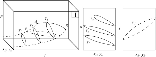
Figure 16.1A. Illustration of a system which does not form an azeotrope. The two-dimensional envelopes correspond to cross sections shown on the three-dimensional diagram. The P-x-y diagrams are vertical cross sections, and the T-x-y is a horizontal cross section.

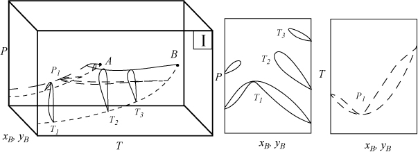
Figure 16.1B. Illustration of a system which forms a minimum boiling azeotrope due to positive deviations from Raoult’s law. The two-dimensional envelopes correspond to cross sections shown on the three-dimensional diagram.

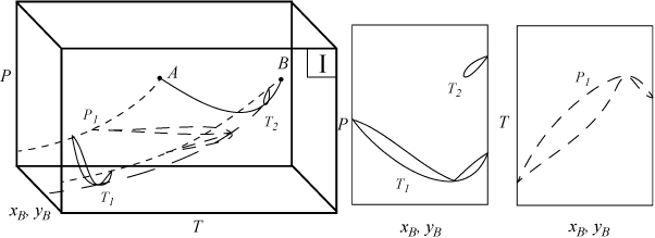
Figure 16.1C. Illustration of a system which forms a maximum boiling azeotrope due to negative deviations from Raoult’s law. The two-dimensional envelopes correspond to cross sections shown on the three-dimensional diagram.

P-x-y and T-x-y diagrams for systems with LLE are shown in Figs. 16.2A and 16.2B. The liquid-liquid behavior occurs in the region to the left of the critical endpoint U, in the U-shaped region above the vapor-liquid envelope. Three-phase llv occurs on the surface marked with tie lines. The intersection of this surface with P-x-y and T-x-y diagrams results in the llv tie lines on the cross-section diagrams. At the upper critical endpoint, U, a vapor and liquid phase become identical, denoted with the notation l–l=v. When the vapor pressures of the components are significantly different from each other, the system may not have an azeotrope as shown in Fig. 16.2A(a–c). When the vapor pressures are closer to each other, azeotropes and heteroazeotropes will form. Fig. 16.2B(d–f) shows a system with heteroazeotropic behavior below the temperature of the upper critical endpoint, T_U, and azeotropic behavior above T_U.

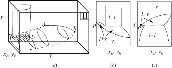
Figure 16.2A. (a) Type II system where the vapor pressures are significantly different; (b) P-x-y at a temperature below T_U; (c) T-x-y at a pressure below P_U.

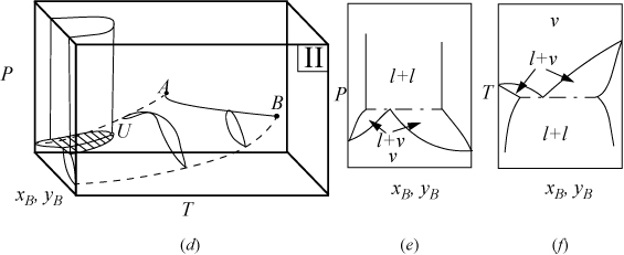
Figure 16.2B. (d) Type II system where the vapor pressures are relatively similar; (e) P-x-y at a temperature below T_U; (f) T-x-y at a pressure below P_U. It is also possible for an azeotrope to lie to the right or left of the liquid-liquid region, rather than the heteroazeotropic behavior that is shown.

Perspective

Before advancing further into the phase behavior classifications, some justification for such study is offered. High pressure can be used to create dense fluids that are useful for processing. For example, high pressure gases are employed industrially for petroleum fractionations in the oil industry and for hops and spice extractions and coffee decaffeination in the food industry. Dense gases are also under study for fractionation of specialty vegetable and fish oil components, as reaction media for polymerizations and other chemical synthesis and separations. High pressure processing and supercritical fluid extraction rely on control of solubility through manipulation of temperature and pressure. Solubility behaviors follow clear patterns which depend on similarities/differences in the thermodynamic and structural properties of the solute and the solvent. This section serves as an overview of phase behavior and systematic trends in phase behavior.

Natural materials such as foods and oils are multicomponent mixtures. Polymers typically contain a molecular weight distribution. Frequently, these types of mixtures are not well identified or characterized. Solubilities and extractabilities for these mixtures are currently difficult to predict quantitatively; however, significant knowledge regarding solubility trends may be obtained by studying simpler binary and ternary systems. Solubility represents a saturation condition; therefore, solubility is represented as a boundary on a phase diagram. Systematic study of binary and ternary systems shows that the phase boundaries of ternary systems are intermediate to the constituent binary systems, and many of the same trends continue in multicomponent systems,² although fundamental exploration of the trends is an ongoing research topic. Process simulators and computers continue to simplify the calculation of phase equilibria; however, the interpretation of the resultant phase behavior is aided by a general understanding of the classes of phase behavior presented in this section.

16.2. Classification of Binary Phase Behavior

Since 1970 there have been several reviews and classifications of phase behavior²,³,⁴,⁵,⁶,⁷,⁸,⁹,¹⁰,¹¹. The types are usually summarized by the projection of their phase boundaries onto two-dimensional pressure-temperature diagrams. Type I and II phase behavior have already been discussed, and they are shown by the upper two plots in Fig. 16.3. Note that azeotropic behavior is a subset of the major classes of behavior and it is not shown explicitly on the projections in Fig. 16.3.

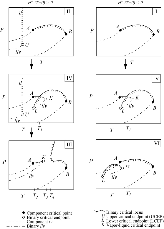
Figure 16.3. Progression of binary phase behavior with increasing molecular asymmetry according to van Konynenburg and Scott.¹⁰ Arrows denote progressions of phase behavior expected by theory. Experimental progressions frequently differ.

For this discussion, the convention of van Konynenburg and Scott¹⁰ is followed for classification of phase behavior. Following a trend that should be familiar by now, van Konynenburg and Scott explored the implications of the van der Waals equation in pursuit of answers to questions like those raised in the introduction. There are six major types of phase behavior shown in the plots which use special notation denoted in the figures and at the end of this section. The types of phase behavior are indicated with the Roman numerals in the upper left of each plot, and the distinctions between the types are due to the location of critical points and critical loci. Types I–V are exhibited by the van der Waals equation at various proportions of size and energy density. Type VI phase behavior appears to be exclusive to aqueous systems.¹¹

The Gibbs phase rule is helpful in interpreting the P-T projections. In a pure system, if two phases coexist, one degree of freedom is available; therefore, two-phase coexistence appears as a line on a P-T projection. At the triple point, solid, liquid, and gas coexist, and no degrees of freedom are available; therefore, the condition is a point on the P-T projection. At critical points, all intensive properties of two phases become identical, so the number of degrees of freedom is reduced, and this also appears as a point for pure systems. To avoid misuse of the phase rule, only intensive variables are used for the degrees of freedom. Also, the intensive variables must be varied over a finite range; for example, two fluid phases are impossible above the critical temperature of a pure substance. More detailed discussions of the correct use of the degrees of freedom are available.¹²

In a binary system, liquid-vapor phase behavior may occur with two degrees of freedom. Liquid-vapor critical behavior occurs with one degree of freedom. Therefore, liquid-vapor behavior appears within a region on the P-T projection, and critical behavior occurs along a line known as the critical locus. In Fig. 16.3, pure component l-v lines are indicated by the dashed lines. Pure component critical points are indicated by solid circles. Invariant critical points in the binary are indicated by open circles and critical lines are indicated by solid lines. Critical lines are hashed to indicate the side on which two phases coexist. Since the critical locus is a projection on the P-T diagram, the diagram and phase rule indicate that two phases coexist on one side of the curve over a finite composition range. The diagram does not imply that two phases will coexist at all compositions below the critical locus. Also, in some areas, two critical curves are superimposed over the same temperature-pressure range (e.g., Types IV and V); however, the overlaps are due to the projection onto the two-dimensional diagram—the two overlapping regions of critical behavior occur over different composition ranges. The critical locus represents conditions where two phases become identical but this does not necessarily imply that only one phase exists above the critical locus because: 1) the two phases which become identical at the critical locus may coexist at temperatures and/or pressures slightly above the critical locus as nonidentical phases (see Example 15.10 on page 601; and 2) if three phases exist below the critical line, two phases will coexist above the critical line. Also, the absence of a critical line on a region of a P-T trace does not imply that only one phase is present; it simply means that no phases become identical within the range of the diagram.

Phase Behavior in the Presence of Solids

Figs. 16.1A–16.5 illustrate only fluid phase behavior. Solid-liquid-vapor coexistence can interfere with the fluid phase behavior when the triple point temperature of the higher molecular weight (heavier) component approaches the range of experiments. (The general trend is for the melting point to increase with molecular weight.) The superposition of solidus lines on these diagrams will be discussed later. For all the phase diagrams sketched here, the light component A, has the lower critical temperature and appears at the left in Fig. 16.3 and in the rear of Fig. 16.4.

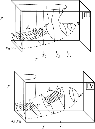
Figure 16.4. Type III and IV phase behavior illustrated on three-dimensional diagrams. Symbols are the same as Fig. 16.3. The labeled temperatures are the same as Fig. 16.3 and are used for plotting cross sections in other figures.

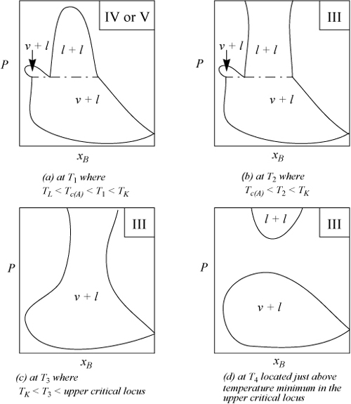
Figure 16.5. Illustration of selected isothermal P-x sections for Types IV, V, and III. Symbols and labeled temperatures are the same as Figs. 16.3 and 16.4.

Molecular Asymmetry

The type of phase behavior depends on the molecular asymmetry of the mixture. Molecular asymmetry is a term used to describe size differences (molecular weight) for functionally similar molecules or polarity or functional differences for molecules of similar molecular weight. As the molecular asymmetry of the system increases, the critical points of the species generally move farther from each other on the P-T traces. With increasing disparity of the critical points, all phase behavior spans increasingly larger areas of P-T space.

Type I and Type II phase behavior occurs in systems where the molecular asymmetry is relatively small. When the molecular asymmetry is greater, the immiscibility regions become larger, as illustrated by the three-dimensional diagrams for Types III and IV in Fig. 16.4. Note that the region below U in Type IV can look the same as the region below U in Type II. Fig. 16.5 shows some isothermal sections where the temperatures used for the plots are denoted in Figs. 16.3 and 16.4. Note that the phase behavior in Figs. 16.5(a) and 16.5(b) differ only in the existence of a ll critical point of the first diagram. The effect of temperature on the phase behavior of a Type III system is interesting because the narrow neck region can pinch off as the temperature is increased, resulting in the cross sections of Figs. 16.5(c) and 16.5(d).

Molecular asymmetry was characterized by van Konynenberg and Scott by the variables along the axes of Fig. 16.6(a). We can refer to Fig. 16.6(a) as a master phase map because it shows where to find certain types of behavior, but it does not provide a system-specific diagram. These must have been extremely painstaking computations in 1970. Fortunately, modern programming makes it feasible to compute phase diagrams with relative ease. A particular example is the GPEC project being developed by Cismondi and coworkers.¹³ We can gain insight into the process required to develop a phase map by running the (free) GPEC program for mixtures of n-alkanes with N₂, CH₄, C₂H₆, CO₂, CH₃OH, and H₂O using the Peng-Robinson equation. To generate a map, each point in Fig. 16.6(b) represents a computation for a different mixture. X represents type II, Δ represents type III, and □ represents type IV. Consider N₂ + n-alkanes. The phase diagram for N₂ + methane is type I, N₂ + ethane is type IV, but N₂ + propane and all higher molecular weight n-alkanes are Type III, based on the calculations. This is expected based on the progressions in Fig. 16.3 (Also, see Assimilation of Experimental Data on Homologous Series on page 629.) Type III behavior may seem somewhat surprising. It means that the vapor-liquid critical locus never quite merges from one pure component to the other. For the N₂ + propane system, the propane-rich critical temperature locus extends below N₂′s critical temperature, but the pressure is higher and it is impossible to squeeze enough N₂ into the propane such that the critical loci connect. Instead, the N₂-propane phase-split widens with increasing pressure into something resembling l + l (Fig. 16.5(c)). The driving force in this case is the high compressibility near the critical region, and the difference in energy density between N₂ and propane. Type IV for N₂ + ethane is peculiar; it exhibits a liquid-liquid phase split, even though neither component is polar.

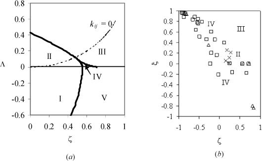
Figure 16.6. Global phase maps (a) for equal sized molecules for the van der Waals equation, after van Konynenberg and Scott. The dashed line corresponds to k₁₂ = 0. (b) Variable sized molecules with the Peng-Robinson equation at k₁₂ = 0.

The axes in Fig. 16.6 are defined such that differences in size, solvation, and energy density are characterized.

where a and b are the van der Waals parameters. Recall from Eqn. 12.21 that a/b² ~ δ².

Several notes should be added to put Fig. 16.6(b) into context. Perhaps the most important observation is that the boundaries between types of behavior are not perfectly distinct. Types IV and III may overlap occasionally depending on the specific components in the mixture. Nevertheless, some general trends are discernible. For example, the range of Type IV behavior appears to be much larger when the molecules vary in size than one might infer from Fig. 16.6(a). Furthermore, it should be noted that, for the Peng-Robinson equation, the ξ – ξ relation increases up and to the left along a homologous series; so the number of components in a series that overlap the Type IV region may be greater than initially anticipated. On a related note, when the molecular weight of the larger molecule exceeds ~500 the mapped points lie in a tiny portion at the upper left corner of the figure. Thus, a vast amount of polymer solution experience lies in a region where Types II, III, and IV are barely distinguishable based on the current analysis, and small variations in k₁₂ would drastically alter the phase behavior (as one might expect in the presence of alcohols, for example). First, Types I and V do not appear although many phase diagrams have been classified as Types I and V experimentally. Similar to van Konynenburg and Scott, we attribute this to interference from solid phase boundaries in the experimental systems (as may become more obvious when studying below), hypothesizing that a ll region must exist at T→0 when the geometric mean is applied. Hence Type II systems may be classified experimentally as Type I if the ll region lies below the solid phase boundary, and similarly for Type IV and V systems.

Phase Stability and Critical Phase Behavior Computations

We have touched on the subject of phase stability previously, but we have not delved deeply into it because it can be a complicated subject if treated in detail. Referring to the critical points of pure fluids, we developed Eqns. 7.27 based on a simple analysis of the inflection behavior of isotherms. A similar analysis led to the identification of spinodal conditions and formulation of the equal area rule as a computational method for vapor pressure in the form of Eqn. 9.49 on page 358. Conceptually, stability analysis is always similar to the perspective developed for pure fluids, but the derivatives become more complicated when the dimensionality of the problem expands to include multiple components.

A hint of the development for mixtures was given in the LLE (l + l) analysis leading to Eqn. 14.7. Once again, we considered the inflection behavior with respect to a single variable (x₁) to infer the necessary conditions for LLE, and, coincidentally, the critical point. If you consider that pressure is the first derivative of the Helmholtz energy, you may be struck by the similarity of Eqns. 7.27 and 14.7. At constant volume, both involve second and third derivatives of “free energy” with respect to mole number.

The multicomponent analysis has been discussed in depth by many authors. The state of the art as of this writing is well represented by the work of Michelsen and Mollerup.¹⁴ Briefly, the extension requires a generalization of the tangent line evident in the LLE (l + l) development to become a tangent plane. This leads to a need for many derivatives with respect to density, mole number, and temperature along with tests for the stability of phases detected. This approach forms the basis of the GPEC program by Cismondi and coworkers.

An alternative formulation has been presented by Eubank and coworkers as an extension of the equal area rule (EAR) for pure fluids.¹⁵ As in the case of pure fluids, stability checking is an inherent part of the EAR method because the integrand is easily checked for extrema before performing further analysis. The formulation of EAR for binary mixtures is particularly simple since it involves only a single variable, x₁.

Note that the right-hand steps are only possible for binary mixtures. From Eqn. 10.42, G = x₁ μ₁ + x₂ μ₂, so

Setting (1 – x₁) = x₂ and rearranging,

This equation facilitates computing (dG/dx₁) using a typical program for chemical potentials. Since μ_i^α = μ_i^β,

To recognize the EAR form, we can multiply by (x₁^α – x₁^β) and expand to obtain

Combining the μ₂ – x₁^αμ₂ = x₂^αμ₂. A similar combination gives x₂^βμ₂. So,

Returning to Eqn. 16.9, substituting and rearranging, we have

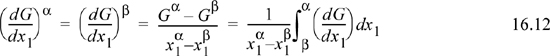
Eqn. 16.12 is analogous to Eqn 9.49 and implementation follows the analogous procedure: Find the spinodals, guess the value of (dG/dx₁)^α, solve for x₂^α and x₁^β, compute the next guess for (dG/dx₁)^α, and repeat to convergence. One practical note for polymer systems would be to search for spinodals based on volume fraction since dG/dΦ₁ = 0 when dG/dx₁ = 0, and using volume fraction spreads the concentration range over more reasonable values for polymer systems. Advantages of the EAR approach include (1) relatively few derivative properties are required; (2) a stability test is an inherent part of the procedure; and (3) convergence is stable, even near the critical point.

Experimental Studies of Homologous Series

One way to understand the progression of phase behavior is to review literature measurements which classify the phase behaviors. Classifications are based on experimental studies and may require revision if additional phase transitions are found to occur.¹⁶,¹⁷ Types I or II occur when the molecules are fairly similar in structure or critical properties. Van Konynenburg and Scott found the van der Waals equation predicted the progression II ⇒ V ⇒ III for increasing molecular asymmetry in systems with an endothermic low-temperature heat of mixing, and they found the progression I ⇒ V for increasing asymmetry in systems with an exothermic low-temperature heat of mixing. Most nonpolar systems are expected to have endothermic heats of mixing (e.g., ethane-butane, benzene-hexane) and might be expected to be Type II by theory; however, they are classified as based on experimental measurements, and most are Type I. Type II phase behavior includes a liquid-liquid immiscibility below the critical temperature of both components. The liquid-liquid behavior is often relatively insensitive to pressure when the liquids are incompressible far below the critical temperature. In the liquid-liquid region, as the temperature is increased, the liquids become increasingly miscible in each other until they become identical at the UCEP. The UCEP occurs at extremely low temperatures for small endothermic heats of mixing, and is frequently not found experimentally due to lack of experimental exploration at low temperatures or due to freezing of the liquids before they become immiscible. While a significant number of liquid-liquid experiments have been performed to locate liquid-liquid UCEPs at atmospheric pressure,¹⁸ phase behavior characterization near the critical point of the lighter component is necessary to permit classification as Type II or IV. A summary of some homologous series is provided below to explore the progressions of phase behavior. To study the series, the asymmetry of the systems is systematically increased by varying the molecular weight of the heavier component by one functional group at a time, and observing the trends in the location of critical points and the class of phase behavior.

Ethane/n-Alkane Series Trends

Studies of the ethane family are summarized by Peters, et al.,¹⁶ and Miller and Luks.⁶, Type I behavior exists up through n-heptadecane because a UCEP has not been reported, possibly because the components freeze before they become immiscible. Beginning with n-octadecane, a liquid-liquid-vapor region develops near the ethane critical point characteristic of Type V. Once again, a UCEP is not found experimentally. This phase behavior continues through n-tricosane. With n-tetracosane and n-pentacosane a modification of Type V or III occurs where the s_Bl₂v line interferes with the fluid behavior as shown in Fig. 16.7(a). The three phase s_Bl₂v line extends from the triple point of the heavier component and intersects the llv line at a quadruple point Q where four phases coexist. Beginning with n-hexacosane, the s_Bl₂v line moves to temperatures above the K point and the Fig. 16.7(d) phase behavior begins.¹⁶ In Fig. 16.7, the line labeled s_Bl₂v denotes the conditions where the solid melts over some composition ranges.⁸ Schneider reports that squalane, a branched C₃₀, exhibits Type III,⁹ which does not fit the pattern of n-alkanes at the same carbon number.

Figure 16.7. Pressure-temperature projections of phase behavior when the triple point of B is in the vicinity of the critical point of A. Symbols are the same as Fig. 16.3, except as noted.

CO₂/n-Alkane Series Trends

Studies of the CO₂ family are summarized by Schneider,^7,9 Miller and Luks,⁶ and Enick et al.¹⁷ Pure CO₂ freezes at a relatively high reduced temperature (T_r = 0.712) while ethane freezes at a comparatively low reduced temperature (T_r = 0.295). Therefore, it may initially seem less likely to observe liquid-liquid immiscibility in CO₂ systems because the systems might freeze before the liquid-liquid critical point, U, is reached; however, the opposite is found, and although the liquid-liquid region is not seen for the lightest alkanes, n-heptane clearly shows Type II behavior.⁶ Type II behavior continues through n-dodecane. Enick, et al.,¹⁷ show that n-tridecane is Type IV, and that beginning with n-tetradecane, the type of Fig. 16.7(a) emerges. Schneider⁹ reports the type of Fig. 16.7(a) for n-hexadecane. The type of Fig. 16.7(a) is exhibited at n-heneicosane¹⁹ and the type of Fig. 16.7(d) appears with n-docosane.⁶,²⁰ Schneider⁹ reports that squalane, a branched C₃₀, is Type III, and as with ethane, varies from the pattern with n-alkanes.

The homologous series of n-alkanes with CO₂ exhibits liquid-liquid behavior at much higher reduced temperatures compared to ethane.²¹ This may be understood by considering the heat of mixing using the propane system as an example. The low temperature heat of mixing is estimated from the van der Waals equation by

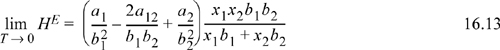
where the a’s and b’s are the van der Waals’ parameters. Using Eqn. 16.13 to approximate the low temperature heat of mixing and the normal van der Waals’ geometric mean combining rule for the cross parameter a₁₂, both the ethane/propane and CO₂/propane systems are endothermic; however, the heat of mixing in the CO₂/propane system is roughly 100 times the heat of mixing for ethane/propane. Therefore, the excess Gibbs energy of mixing will also be considerably larger and liquid-liquid behavior is expected to occur to higher temperatures. In general, the n-alkane series with CO₂ shows greater asymmetry than the same ethane series, as might be expected. Therefore, the solubilities are lower at a given temperature and pressure, and the progression of behavior from Type II to the type of Fig. 16.7(d) occurs at lower carbon numbers, even though the critical temperatures of ethane and CO₂ are approximately the same.

CO₂ and N₂O Series Trends

CO₂/alcohols: Schneider⁹ reports 2-hexanol and 2-octanol as Type II and 2,5-hexanediol and 1-dodecanol⁷ as Type III. As expected, the addition of hydroxyls on component B increases the asymmetry of the system and the same carbon number by raising the critical point of B, and lowers the carbon numbers for transitions between the phase behavior types.

CO₂/aromatics and ethane/aromatics: Both CO₂ and ethane have been studied with n-alkylbenzenes through C₂₁ and C₂₀, respectively.⁶ The over-all trends in behavior are very similar to the comparisons made in the n-alkane series. Polycyclic aromatics have also been studied, and are typically the type of Fig. 16.7(d).⁸

N₂O/n-alkanes: Nitrous oxide has been studied with the n-alkanes, and the phase behavior is very similar to the ethane series³ in both the carbon number where phase behavior changes, and the critical endpoint temperature values.

CO₂/triglycerides/fatty acids: Many common triglycerides and fatty acids are solids at 30°C, and thus exhibit the type of Fig. 16.7(a) or Fig. 16.7(d) behavior in binaries with CO₂. Compounds which are normally liquids will probably be Type III, IV, or V. Relatively few studies of model systems are available and in all studies only solubilities are reported.²²,²³,²⁴,²⁵ Bamberger, et al.²⁵ did determine that lauric and myristic acid, trilaurin, and trimyristin melted at the average pressure of their experiments, but the experiments were insufficient to characterize the phase behavior types as Fig. 16.7(a) or (d). Tripalmitin is reported to remain a solid although the triple point is only 5°C greater than trimyristin. Also, most of the mixtures involving tripalmitin were reported to remain solid, which would not be expected if the solids formed an eutectic mixture.⁸ The other publications have not provided any characterization of the melting behavior of the solids. Unfortunately, disagreements of up to an order of magnitude exist in a few of the solubility measurements. The disagreements have been attributed in part to purity of materials.^23,24 Nilsson, et al.²⁴ report solubility data for mono- and di-glycerides. One interesting conclusion from the analysis of Czubryt, et al.²⁶ is that stearic acid appears to be dimerized in the CO₂ phase. Phase behavior of oil mixtures will be discussed in the section regarding solubility behavior.

Propane/Triglycerides/Fatty Acids Series Trends

Hixson, et al. published most of the available information on these systems in the 1940’s,²⁷,²⁸,²⁹ and recently, more complete information has been published on the propane/tripalmitin system.³⁰ Propane refining of oils was practiced industrially as the Solexol process and descriptions are available.³¹ Similar to the case of stearic acid in CO₂ discussed above, the acids appear to dimerize in the fluid phase. This hypothesis is supported by the correlation of phase behavior with the effective molecular weight, which is double the molecular weight of an acid and equal to the molecular weight of an ester or triglyceride. (See the trend for the LCEP in Fig. 16.8). Binary mixtures of propane with lighter molecular weight acids and esters is Type I (a UCEP has not been located), while the triglycerides and heavier acids and esters exhibit Type IV. For lauric acid (effective M.W. = 400.6) and for myristic acid (effective M.W. = 456.7) a lower critical end point (LCEP) has not been located at propane concentrations between 25 and 95 wt%.²⁹ Tricaprylin (M.W. = 470.7) and higher molecular weight compounds exhibit Type IV. The correlation in Fig. 16.8 is based on only saturated and mono-unsaturated compounds. Conjugation of unsaturation may have a dramatic effect as exhibited by abietic acid which does not show an LCEP above 30°C.²⁸

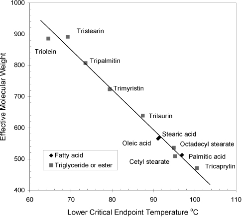
Figure 16.8. Trend in the lower critical endpoint (LCEP) for components in binary mixtures with propane (Type IV systems).

The Solexol process is based on refining of the oils using the llv region in Type IV or V systems between the LCEP and the vapor-liquid critical endpoint, K. The phases of interest are the two liquid phases, and Hixson and coworkers did not measure the vapor phase solubilities. As might be expected, the compounds with the lowest effective molecular weight have the greatest solubility in the propane-rich liquid, and for a given chain length solubility increases with decreasing effective molecular weight: triglyceride - fatty acid - ester. Hixson’s studies concentrate on the measurement of l-l solubilities on the three-phase llv line in binaries and extension of the measurements to model ternary systems. Hixson’s publications address the incorporation of staged countercurrent flow, the importance of density differences for counter-current flow, and internal column recycle using temperature gradients which have been discussed recently in applications with CO₂ extractions.³²,³³ These engineering concepts remain important in industrial applications of high pressure technology. In the Solexol process, virtually all the feed oil leaves the top of the first tower dissolved in propane, and the stream is then fractionated by molecular weight and saturation. The majority of color bodies leave the bottom of the first column. The conjugated unsaturated components are in general less soluble than the saturated or mono-unsaturated components. One of the distinct capabilities of the Solexol process was the concentration of vitamin A but, as alternative methods for obtaining vitamin A became available, the process was abandoned.

Assimilation of Experimental Data on Homologous Series

Schneider⁷ suggests that Types II, IV, and III follow a trend which can be understood if the phase behaviors are considered as a result of effects that are superimposed on each other and can be best visualized on Fig. 16.3. When a homologous series of systems is studied, with only the heavier compound varying, the first system to exhibit Type III behavior has a strong maximum and minimum in the critical line extending from the heavier component critical point. If this strong minimum exists for less dissimilar systems, it is expected to intersect the llv line in two places, giving Type IV behavior. These trends also appear consistent with the calculations of Chai³⁴ using the Peng-Robinson equation. Another trend is obvious which supports this theory. As the dissimilarity of components increases, the UCEP temperature at U increases which tends to decrease the difference in the temperatures of U and L of Type IV systems until they merge and Type III results (Fig. 16.9). It is also possible for the phase behavior to progress directly from Type II to Type III.¹⁰

Figure 16.9. Illustration of trends in critical endpoint temperatures as the molecular asymmetry of systems increases for carbon dioxide + n-alkyl benzenes (diamonds, triangle, filled circles) and carbon dioxide + n-paraffins (x’s, o, filled squares) as compiled by Miller and Luks.¹¹ In both series, the systems are Type II below C13, Type IV for C13, then Type III above C13.

Critical Phase Behavior Summary

Phase behavior is determined by the degree of molecular asymmetry. A range of phase behavior exists, and a natural progression of phase behaviors occurs as the asymmetry of the system is increased. This progression can be visualized with two-dimensional master phase maps that represent sections through a three-dimensional space characterized by asymmetry in size, solvation, and energy density. These asymmetries can explain five of the six types of phase diagram observed in nature. The sixth type of diagram seems to be peculiar to aqueous systems and presumably may require explicit accounting for hydrogen bonding. Trends in critical phase behavior suggest that organic acids dimerize in nonpolar solvents.

P-T projections are specific to the type of phase behavior and summarize conditions where various processes are feasible or infeasible.

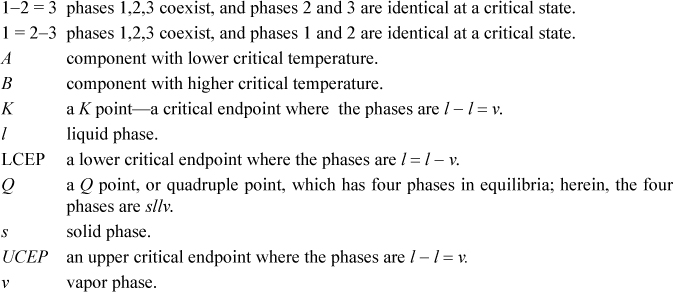
List of Special Symbols for This Section

16.3. Residue Curves

Distillation is among the most highly developed and reliable separation techniques for the chemical industry, so it is usually among the first separation techniques considered during process design. Design of multicomponent distillation columns can be complicated by azeotropes and heteroazeotropes. Shortcut distillation techniques are useful for distillation column screening, but azeotrope systems require modified shortcut equations and relative volatilities.³⁵ Design of multicomponent steady-state distillation columns is usually performed by process simulators; nevertheless, many design hours are saved if the phase behavior is explored using residue curves before working with the detailed column calculations. In this section, residue curves for ternary systems with a single feed and one distillate product and one bottoms product will be covered.³⁶ Residue curve analysis for ternary systems, under these conditions, involves the following concepts that will be described below.

1. The steady-state column feed, distillate, and bottoms compositions are co-linear on ternary diagrams in accordance with the lever rule.

2. Two combined streams may be represented by a mixing point co-linear with the feed streams at a point between the streams given by the lever rule.

3. Binary and ternary azeotropes are connected on ternary diagrams by boundary lines called separatrices. (A single boundary is called a separatrix.)

4. Separatrices divide the ternary residue curve map diagram into regions.

5. As a reliable rule, the distillate, feed, and bottoms compositions will all be in the same residue curve map region.³⁷

6. Residue curves begin and end in a single region—they do not cross separatrices.

Therefore, only certain composition regions in a ternary system describe possible products for a given feed, and the residue curves provide the guide to attainable compositions.

Residue curves represent the trace of liquid-phase (the residue) composition during a single-stage constant-pressure batch distillation. Single-stage batch distillation calculations are not complex, and will be introduced below using the VLE K-ratios that have been the topics of earlier chapters. As the batch is distilled, the boiling point of the residue will increase until the composition reaches either a maximum boiling azeotrope or the pure composition of the highest boiling component. The residue curves will terminate at these compositions. The residue compositions will move away from any minimum boiling azeotropes and/or the pure composition of the lowest boiling component. The residue curves originate at these compositions. In the diagrams in this section, we use the letter o to represent the low boiling point residue curves’ origin and the letter t to represent the high boiling point residue curves’ terminus.

The Bow-Tie Approximation

Let us begin analysis by considering residue curves for a ternary system without azeotropes, propane + butane + pentane. As this ternary mixture boils, bubble-point calculations show that propane and butane are the most prevalent vapor species. As the vapor is removed, the residue becomes increasingly rich in pentane. Residue curves calculated with the Peng-Robinson equation are shown in Fig. 16.10(a). Starting from any initial composition, the curves on the diagram can be used to follow the trace of the residue composition. The residue from any ternary composition in this system will become increasingly rich in pentane. The residue curve map has a single region, and the residue curves originate at pure propane (the lowest boiling composition in the region) and terminate at pentane (the highest boiling point in the region). Residue curves are helpful in the design of steady-state continuous flow distillation columns because the accessible compositions of distillate and bottoms products from a steady-state distillation column can be found by studying the region of the residue curve map that contains the feed. The distillate of a one-feed steady-state column will tend to approach the origin of the residue curves, and bottoms of the column will tend to approach the terminus of the residue curves within the restrictions summarized in points (1) through (6) above.

Figure 16.10. (a) Residue curves for the system propane + n-butane + n-pentane as calculated with the Peng-Robinson equation at 1 bar; (b) methanol + acetone + water as modeled with the UNIQUAC equation at 1 bar; (c) methanol + ethanol + benzene as modeled with the UNIQUAC equation at 1 bar. Calculations performed using Aspen Plus ver. 9.2.

Recognize the importance of point 1, that the feed, distillate, and bottoms for a ternary system must be colinear when plotted. Consider the implications for the propane + butane + pentane system shown in Fig. 16.10(a). When a column is designed for a specified feed, F, the distillate or bottoms composition may be specified also, but not both. For a feed, F, if the bottoms product of a distillation column is B₁, the distillate (top product), D₁, must also be colinear on the plot, and F must fall between B₁ and D₁ to satisfy the lever rule material balance, D₁/F + B₁/F = 1, and . Another option for operating the column is to achieve pure propane distillate, D₂. In this case, the feed must lie on a line between D₂ and B₂. The first approximation of reachable compositions is given by the bow-tie shaped region D₁-D₂-B₂-B₁.³⁸ The distillate and bottoms compositions are not required to be on the boundary of the region as we have chosen to show in the figures, but the colinearity and lever rule must be followed. Note that it is not possible to simultaneously obtain pure propane and pure pentane in a single-feed, two-product (distillate and bottoms) column from feed F. Note that products near pure butane are unattainable, so design can focus on other alternatives. The bow-tie shaped region is an approximation that will be adequate for the screening introduction intended here.

Azeotropes

When one azeotrope exists in a ternary system, the residue curve map will still be a single region, but the azeotrope will be an origin or a terminus for the residue curves. Maximum boiling azeotropes may become the terminus of some residue curves, and minimum boiling azeotropes may become the origin of some residue curves. For example, in the methanol + acetone + water system shown in Fig. 16.10(b), the methanol + acetone system forms a minimum boiling azeotrope that becomes an origin for the residue curves because it is the lowest boiling point in the region. The distillate product for any steady-state column with a feed in the region will tend toward this composition. The highest boiling point in the region is the terminus of the residue curves at the composition of pure water, and the steady-state column bottoms will tend toward this composition. The bow-tie approximation of attainable compositions is shown for a feed F, and note that a distillate composition of pure methanol or pure acetone is not attainable because the residue curves’ origin is the azeotrope. The lever rule concepts apply as in nonazeotropic systems.

When two or more azeotropes exist, the residue curve map will often be divided into two or more regions of residue curves. The residue curve maps show the distillation regions of attainable compositions, and the location of the separatrices. For example, residue curves for methanol + ethanol + benzene are shown in Fig. 16.10(c). In the left region, ethanol is the high boiling point (residue curve terminus) and the methanol + benzene azeotrope is the low boiling point (residue curve origin). In the right region, the methanol + benzene azeotrope is also the residue curve origin (low boiling point) and benzene is the residue curve terminus (high boiling point). The ethanol + benzene azeotrope is at an intermediate temperature between the origin and terminus of each region, and therefore, is neither an origin nor a terminus, and is called a saddle point. Two different arbitrary feed compositions are plotted on the diagram, and the corresponding bow-tie shaped regions of approximate accessible compositions are shown. Since the design rule is that a single column cannot cross a separatrix, the practical boundary for distillate compositions from the feed F₁ is approximated by the region F₁-D₁-D₂. For a feed of composition F₂, the practical region of attainable distillate compositions is approximated by the region F₁-D₁-D₃. Although an example with a maximum boiling azeotrope is not shown, systems with these azeotropes can be screened using the same lever rule techniques; however, the bottoms of the column will be affected by the azeotropes.

Heteroazeotropes — Systems with LLE

Ternary systems exhibiting LLE form minimum-boiling heteroazeotropes and can often be separated in a system of two columns as shown in Fig. 16.11. The LLE behavior often spans a separatrix on the residue curve map. This means that an overhead stream, D_M, can be condensed in a decanter, and one of the liquid phases will be on the same side of the separatrix as D₁ and can be returned into that column (left in the figure). The other decanter liquid phase will be on the other side of the separatrix and can be used as a feed to another column (right in the figure). An example of this procedure is given by the separation of ethanol + water using benzene. In this case, benzene is intentionally added to break the azeotrope and permit water to be recovered from one column and ethanol from the other column. The system involves an ethanol + benzene minimum boiling azeotrope, an ethanol + water minimum boiling azeotrope, and a benzene + water minimum boiling heteroazeotrope. The system has three separatrices. The ternary azeotrope, o, is the lowest boiling point in the system and it is the origin of the residue curves for all three regions. The left column operates in the right region of the residue curve map, and the right column operates in the upper left region. Care is taken to avoid having F₂ fall in the lower left region of the residue curve map; such a feed would result in a bottoms of benzene rather than ethanol. Illustrative material balance lines are provided on the diagram, and the LLE curve is superimposed on the residue curve map to clearly show how the tie lines span the separatrices. For this example, the residue curve origin can be moved farther into the LLE region by increasing the system pressure.

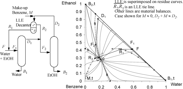
Figure 16.11. Illustration of the column configuration, residue curves, and LLE behavior for the separation of ethanol and water using benzene. Residue curves calculated using Aspen Plus ver. 9.2 with UNIQUAC at 760 mmHg, LLE data at 25°C from Chang, Y.-I., Moultron, R. W. 1953. Ind. Eng. Chem. 45:2350. LLE tie lines are not plotted to avoid clutter, but tie-line data are represented by pairs of points along the binodal line.

Generating Residue Curves

Residue curves are generated by a bubble-temperature algorithm for a simple single-stage batch distillation without reflux. If the total moles vaporized from a multicomponent mixture is dn^L, the moles of component i leaving are calculated by the composition of the vapor phase, dn_i = y_idn^L. For component i in the liquid phase, dn_i = d(x_in^L) = n^Ldx_i + x_idn^L. Equating the vapor and liquid expressions for dn_i,

Rearranging,

which may be written

where K_i values can be calculated by any appropriate bubble-temperature method from Chapters 10–14 for the system at composition x_i. To generate residue curves in an N-component mixture, differential values of d(ln[n^L]) may be chosen arbitrarily to generate differential values of dx_i. Only N – 1 values of dx_i are required since

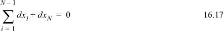
From an arbitrarily selected initial composition, the trace of x_i values yields the residue curve. Special care should be taken to include liquid-liquid behavior, if present in the system, requiring a three-phase bubble-temperature calculation as illustrated in Chapter 14. Table 16.1 presents the first few residue curve calculations for the n-pentane(1) + n-hexane(2) + n-heptane(3) system at 0.1013 MPa via Eqn. 16.16 using the shortcut K-ratio method to calculate the K_i values. The initial composition for the residue curve is arbitrarily selected as x₁ = 0.1, x₂ = 0.6 and x₃ = 0.3 denoted in cells with double ruling in Table 16.1. The step size for Eqn. 16.16 is arbitrarily selected as d(ln[n^L]) = –0.15 to generate the dx_i values listed in the table. Eqn. 16.16 is used directly as a finite difference formula to provide a quick estimate as x_i^new = x_i^old + dx_i^old to move down the table from the initial point. The residue curve is generated towards the increasing n-pentane liquid compositions by moving up the table from the initial point and using x_i^new = x_i^old – dx_i^old. More accurate finite difference methods can be employed for important applications. Residue curves are calculated in other composition ranges by selecting other initial compositions. The location of the separatrices is obvious after generating enough residue curves. Residue curve calculations are offered by some process simulation software due to the importance of screening separations in the chemical industry. More detailed discussions are available.³⁹

Table 16.1. Example Calculation of Residue Curves for n-butane(1) + n-hexane(2) + n-heptane(3) as Predicted by the Shortcut K-ratio Method

Residue Curve Summary

Residue curves provide useful tools for designing separation schemes. Although a single feed column with one overhead and one bottoms product cannot cross a separatrix, a separation scheme can be constructed using multiple columns to achieve most separations. The residue curve maps are useful in screening additives for selection of the most promising systems. Residue curve calculations for homogeneous liquids are straightforward, and an algorithm has been presented.

16.4. Practice Problems

P16.1. Consider the methanol(1) + water(2) + acetone(3) system with a feed shown in Figure 16.10(a). Rate each of the following products as impossible or possible, and explain.

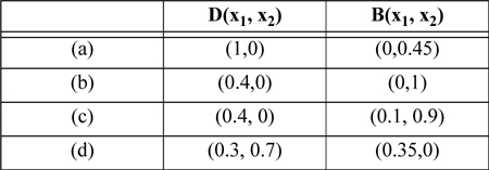
(ANS. impossible; impossible; possible; impossible.)

16.5. Homework Problems

Phase Behavior

16.1. A binary mixture obeys a simple one-term equation for excess Gibbs energy, G^E = Ax₁x₂, where A is a function of temperature: A = 2930 + 5.02E5/T(K) J/mol.

a. Does this system exhibit partial immiscibility? If so, over what temperature range?

b. Suppose component 1 has a normal boiling temperature of 310 K, and component 2 has a normal boiling temperature of 345 K. The enthalpies of vaporization are equal, both being 4475 cal/mol. Sketch a qualitatively correct T-x-y diagram including all LLE, VLE behavior at 1 bar.

16.2. As the research scientist of a company where phase equilibria is under study, you are approached by a laboratory technician with the most recent (and incomplete) high pressure phase equilibria results. The technician expresses concern that the data have not been collected correctly, or that some of the samples may have been mislabeled for some of the runs, or there is a problem with the automated equipment, because the data appear different from what he has seen before. The most recent results are summarized on the two P-x-y diagrams over the same P range shown below at T₁ and T₂, where T₁< T₂. The circles and triangles give coexisting phase compositions at each pressure. What is your response?

16.3. Using the value k_ij = 0.084 fitted to the system methanol(1) + benzene(2), use the Peng-Robinson equation to plot P-x-y behavior of the system at the following temperatures: 350 K, 500 K, 520 K. Plot the T-x-y behavior at the following pressures: 0.15 MPa, 2 MPa, 5.5 MPa. Sketch the P-T projection of the system.

16.4. Use UNIFAC to model the methanol(1) + methylcyclohexane(2) system. Provide a P-x-y diagram at 60°C and 90°C, and a T-x-y at 0.1013 MPa.

16.5. Use UNIFAC to model the methanol(1) + hexane(2) system. Provide a P-x-y diagram at 50°C and 25°C, and a T-x-y at 0.1013 MPa.

16.6. Model the system CO₂(1) + tetralin(2) using k_ij = 0.10. Generate a P-x-y diagram at 20°C, 45°C, and a T-x-y at 12 MPa and 22 MPa. What type of phase behavior does the system exhibit?⁴⁰

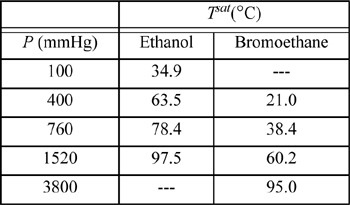
16.7. The system ethanol(1) + bromoethane(2) forms an azeotrope containing 93.2 mol% bromoethane and having a minimum boiling point of 37.0°C at 760 mmHg. The following vapor pressure data are available:

a. Use all of the available data to determine coefficients for equation log₁₀ P^sat = A + B/T by performing a linear regression to find the coefficients A and B. Be sure to use temperature in Kelvin.

b. Use the azeotropic point to determine the parameters for the van Laar equation.

c. Generate a P-x-y diagram at 100°C. Tabulate the data used to plot the diagram.

d. Generate a T-x-y diagram at 760 mmHg. Assume that the activity coefficients are independent of temperature over the range of temperature involved. (This is the type of calculation necessary for generating an x-y diagram for a distillation at 760 mmHg.)

e. Experimentally, the system is found to have a homogeneous maximum pressure azeotrope (Smyth, C.P., Engel, E.W. 1929. J. Am. Chem. Soc., 51:2660). How does this compare with your findings?

16.8. Benzaldehyde is known in the flavor industry as bitter almond oil. It has a cherry or almond essence. It may be possible to recover it using CO₂ for a portion of the processing. Explore the phase behavior of the CO₂(1) + benzaldehyde(2) system, using the Peng-Robinson equation to categorize the system among the types discussed in this chapter. Experimental data are not available, so use an interaction coefficient k_ij = 0.1, which has been fitted to the CO₂-benzene system. Calculate P-x-y diagrams at 295 K and 323 K. Also determine T-x-y diagrams at 34.5 bar and 206.9 bar. Note that 34.5 bar is below the critical pressure of both substances. If a bubble calculation fails, try a dew, and vice versa.

Residue Curves

16.9. For the systems specified below, obtain residue curve maps and plot the range of possible distillate and bottoms compositions for the given feeds. UNIQUAC parameters are provided.

a. methanol(1) + ethanol(2) + ethyl acetate(3), z₁ = 0.25, z₂ = 0.25, r = [1.4311, 2.1055, 3.4786], q = [1.432, 1.972, 3.116], a parameters (in K); a₁₂ = –91.226, a₂₁ = 124.485, a₁₃ = –74.2746, a₃₁ = 389.285, a₂₃ = –31.5531, a₃₂ = 183.154.0
Note: Aspen 2006 gives poor VLE using LLE parameters for this system. Use the provided parameters.

b. Solve part (a), but use z₁ = 0.4, z₂ = 0.4, z₃ = 0.2.

c. methanol(1) + 2-propanol(2) + water(3), z₁ = 0.2, z₂ = 0.6, z₃ = 0.2, r = [1.4311, 2.7791, 0.92], q = [1.432, 2.508, 1.4], a parameters (in K); a₁₂ = 39.717, a₂₁ = –26.6935, a₁₃ = –112.697, a₃₁ = 176.077, a₂₃ = 151.061, a₃₂ = 55.1272.

d. Solve part (c), but use z₁ = 0.6, z₂ = 0.2, z₃ = 0.2.

e. methanol(1) + ethanol(2) + benzene(3), z₁ = 0.25, z₂ = 0.25, z₃ = 0.5, r = [1.4311, 2.1055, 3.1878], q = [1.432, 1.972, 2.4], a parameters (in K); a₁₂ = –91.2264, a₂₁ = 124.485, a₁₃ = –27.2253, a₃₁ = 559.486, a₂₃ = –42.6567, a₃₂ = 337.739.

f. Solve part (e), but use z₁ = 0.4, z₂ = 0.4, z₃ = 0.2.

16.10. Consider an equimolar mixture of methanol(1) + water(2) + acetone(3). Demonstrate that it is not possible to obtain pure acetone as distillate from a single-feed column by generating a residue curve map and applying the bow-tie approximation.⁴¹ What compositions are attainable from this feed? Data: r = [1.4311, 0.92, 2.5735], q = [1.432, 1.4, 2.3360], = a parameters (in K); a₁₂ = –112.697, a₁₃ = –50.9396, a₂₁ = 176.077, a₂₃ = 29.1681, a₃₁ = 218.872, a₃₂ = 228.990.