6. Exploring Data with Simple Charts
The greatest value of a picture is when it forces us to notice what we never expected to see.
—John W. Tukey, Exploratory Data Analysis
The famous statistician John W. Tukey once wrote that exploring data is “graphical detective work.”1
1 These are the first lines in Tukey’s 1977 classic Exploratory Data Analysis.
Tukey created an entire branch of data analysis almost singlehandedly. He called it exploratory data analysis. He explained that, before you can even begin testing your ideas against the evidence, it’s essential to get a good feel for what your data look like. And the best way of doing so involves graphical displays, not just numerical summaries.
It would be presumptuous on my part to assume that I can explain everything about how to explore data. For that, you’ll need to refer to the bibliography at the end of each chapter. However, I’d like to at least give you a glimpse of how it works and how exciting it can be. If you’ve ever thought that statistics is boring,2 get ready for a pretty pleasant surprise.
2 I hated statistics when I was in college. I later came to believe that this happened because some teachers tend to focus just on the more formal side of its methods rather than explaining the underlying logic of those methods, which is a much more interesting approach.
Before we start, some advice: there’s no better way of learning than doing. Think of a subject you care about and find data related to it. I’m interested in poverty, inequality, and educational attainment, so I’ll be exploring related data sets in the following pages. In your case, it can be sports, science, the environment, politics, or whatever. It won’t be hard to find tons of good data in the websites of governmental institutions, international organizations (the UN, the World Bank, the IMF, and so on), and even private companies.
Most of the data I’ll be using can be found on my website, www.thefunctionalart.com. The simple calculations I’ll discuss can be done in a few minutes with any decent software tool like LibreOffice or R (which are both open source and free), Tableau, Microsoft Excel, Apple’s Numbers, JMP, and others. I’ve used R, Tableau, and Adobe Illustrator myself. On my website you’ll also find video tutorials in which I explain how to design some of the charts in this book.
The Norm and the Exceptions
The process of visually exploring data can be summarized in a single sentence: find patterns and trends lurking in the data and then observe the deviations from those patterns. Interesting stories may arise from both the norm—also called the smooth—and the exceptions.
Let’s begin with a simple data set. Every two years, the Brazilian Ministry of Education releases the Ideb, an index that measures quality in basic education in the country. The Ideb, a score between 0 and 10 assigned to each school, is based on formulas that take into account factors like infrastructure, teacher training, student tests, and so on.3
3 Read more about the Ideb here: http://portal.inep.gov.br/web/portal-ideb (use Google Translate if you don’t understand Portuguese).
On a slow, boring Sunday a few weeks ago, I downloaded the 2009 Ideb scores. Why 2009? That was the year I moved to Brazil, where I lived until 2012, so the answer is just sheer curiosity. The spreadsheet, which you can partially see in Figure 6.1, has 19,387 rows, so it’s hardly something you can extract meaning from by eyeballing it, unless you’re some sort of replicant from Blade Runner.
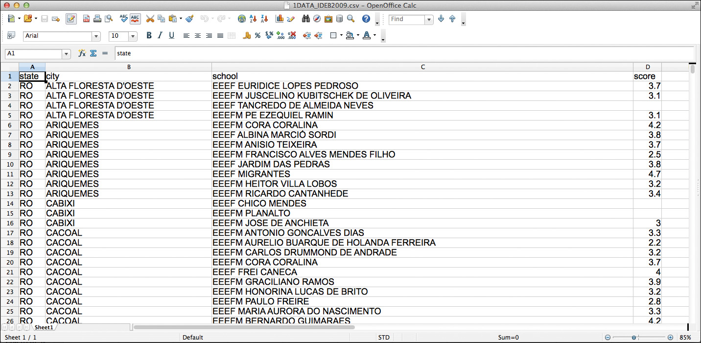
The last column of the spreadsheet is the Ideb score. To refer to all values together I’ll use the term distribution.
OK, we’ve got the data. Now, where to begin?
The Mode, the Median, and the Mean
Insights can arise simply by calculating measures of central tendency. In exploratory data analysis, these are sometimes called the level of the distribution, as they give you an idea of the average size of your numbers and of what their center point is.4
4 I’m following B. H. Erikson’s and T. A. Nosanchuk’s Understanding Data (1992) in this section.
The simplest measure of central tendency is the mode. The mode is the value that appears most often in your distribution. Imagine that these are our Ideb scores:
1.2, 1.4, 1.8, 2.1, 2.1, 2.4, 2.7, 3.6, 3.8, 3.8, 4.0, 4.0, 4.0, 4.1, 4.5, 4.8, 4.9, 5.2, 5.6
The mode, highlighted above, is 4.0. That’s the score that appears the most often. It appears three times. As it turns out, 4.0 also happens to be the mode of the Ideb variable in the actual data set.
Distributions that have just one mode are called unimodal. It may happen that two or more scores are equally—or nearly equally—common, in which case we’d talk about a bimodal, trimodal, or even multimodal distribution.
The second statistic5 we can calculate is the median. This is the value that divides our values in two halves. Going back to the scores before:
5 A brief note on terminology: a number that summarizes or describes an entire population is usually called a “parameter.” If we then draw a sample of that population and calculate exactly the same number—its mean, for instance—we have a “statistic.” For the sake of brevity, I will use just the word “statistic” in this chapter.
1.2, 1.4, 1.8, 2.1, 2.1, 2.4, 2.7, 3.6, 3.8, 3.8, 4.0, 4.0, 4.0, 4.1, 4.5, 4.8, 4.9, 5.2, 5.6
There are 19 scores in that list. Therefore, the median will be the score that has nine scores below and nine above. That position in the distribution is occupied by 3.8, so that’s our median.6
6 A note of caution is needed: the Brazilian Ministry of Education doesn’t calculate the mode, median, or mean for all scores together. They first divide the schools into grades and calculate measures of central tendency for each of them. If you find the 2009 data, you’ll see that there are discrepancies between what’s shown in this book and the official statistics. When in doubt, trust their figures, not mine.
The mean, commonly known as the “average,” is the result of adding up all the values and dividing the result by the total count. In other words:
Mean = Sum of all values / Total count of values
When describing a distribution, you can easily calculate the mode, the median, and the mean, but which one should you report, if you were to report just one? It depends. What you need to remember is that the mean is very sensitive to extreme values, while the median is not. The median is a resistant statistic.7
7 John Tukey was an advocate for the use of resistant statistics in exploratory data analysis. I’ll explain how to use resistant statistics (like the median and quantiles) and non-resistant ones (like the mean and the standard deviation).
To understand the notion of resistant statistics, imagine that you’re analyzing the historical starting salaries of people graduating from the University of North Carolina at Chapel Hill. You calculate the mean of all students, and you discover that geography alumni make a whopping average of nearly $740,000 a year. Now, that’s interesting!
But it’d be hardly a surprise if you knew that Michael Jordan, the basketball player, was a geography major at UNC decades ago.8 His initial salary was probably in the millions of dollars, compared to the few tens of thousands that his peers made. That distorts the mean. Michael Jordan’s salary is an outlier, a value that is so far from the norm—the level of our distribution—that it twists our understanding of the data if we aren’t careful enough.
8 I was a professor at UNC-Chapel Hill between 2005 and 2009. Someone told me a story similar to this one, although I don’t remember the exact figures. Apparently, this calculation was done once, to the amusement of students and administrators alike.
Imagine that these were the first-year annual salaries of all geography graduates from UNC-Chapel Hill, in 2015 U.S. dollars:
$20,000, $22,000, $25,000, $30,000, $32,000, $40,000, $5,000,000
The mean of the series is $738,428. On the other hand, the median, which is the value that divides the salary distribution in half ($30,000), is a much better summary. As B. H. Erickson and T. A. Nosanchuk wrote in their book Understanding Data, when exploring variables like salaries and incomes, you shouldn’t focus on how much people earn on average but on how much the average person earns. If you read that sentence again, you’ll notice that it isn’t a pun.
We say that the median is resistant because even if we added one outrageous value at the lower end of the series of values—say, 10 bucks a year—or increased Michael Jordan’s annual salary to 100 billion dollars, the median would remain untouched, while the mean would go bananas.
Comparing the median to the mean and noticing that they differ a lot is one of the first warning signs of a skewed distribution. In the case of the Ideb scores I’m playing with right now, the median of all schools is 3.8 and the mean is 3.78, so they are almost identical. If we round the mean up, the result will also be 3.8.
Weighting Means
Before we continue, let me make an aside about how careful we need to be when calculating these very simple measures and how important it is to understand our data well before we manipulate them.
Imagine that the Ideb wasn’t an index assigned to each school by one of the branches of the Ministry of Education, based on weighing different factors. Instead, let’s suppose that the score for each school is the result of calculating the mean of the grades that all students in that school get in a certain test. If we wanted to obtain the national mean (a mean of means, also called a grand mean), it would be risky to average the school scores.
To understand why, see Figure 6.2, where we are comparing four schools of different sizes.

School 1 is the largest (10 students), and School 4 is the smallest, with just three students. We can first obtain the mean for each school. Then we calculate the mean of school means. The result is 4.01.
If, instead, we calculate the mean of all students together, regardless of the school they attend, the result is 3.82.
Why do we get this discrepancy? There are a lot of students in School 1, and most of them performed rather poorly in the test. By calculating the mean of each school and then the grand mean of all schools, rather than the mean of all students, small schools are given the same weight as bigger schools. Calculating a grand mean—a mean of school means—would be appropriate only if all schools had a similar number of students.
But what if it’s impossible to access the entire data set of millions and millions of test grades, one per student? In that case, we need to take school size into consideration to calculate a weighted mean. The formula for this is shown in Figure 6.3. Remember it the next time you need to calculate mean scores of groups of different sizes—schools, cities, counties, states, countries, or whatever. And be aware that this is one of the many techniques used by people who are fond of lying with statistics.

Range
Calculating the median, mean, and mode is a good place to start when exploring data. Sometimes, they alone will lead you to interesting stories. But they won’t be enough in most cases.
The challenge we face if we just rely on measures of central tendency to summarize our data is that we don’t really know if most values in our data set are close to them or if they are widely spread apart. This is critical information.
In the case of the Ideb, we could first look at the highest and the lowest values. The difference between the maximum and the minimum value of a distribution is called the range. Figure 6.4 shows it, along with all other statistics we have found so far, and a new one: the 6.0 minimum goal that the Brazilian government wants most schools to achieve in the future.
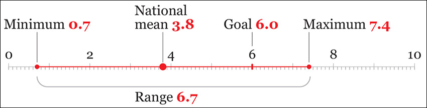
We now know that there are some terrible schools (0.7!) and some very good ones. But how many bad and good schools are there, really? How many are clustered around the national mean? And how many are close to the 6.0 goal or even surpass it?
To find out, we need to take a more detailed look at our data. Let’s create a plot that shows how many schools have obtained good and bad scores. It will also reveal the shape of our distribution. We call this a histogram (Figure 6.5). In a histogram, values are aggregated into bins—ranges of Ideb scores, in this case. In Figure 6.5, the bins have a range of 0.1 score-points.
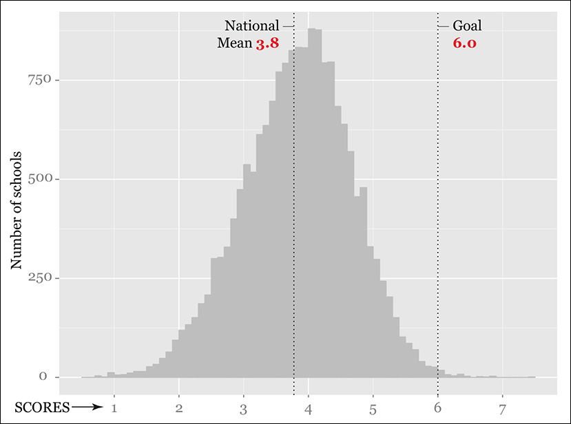
In a histogram, the height of each bar corresponds to the number of records or scores (school counts here) within each bin. A histogram is intended to show the frequency of each value, or of groups of values, within a data set. The higher the bar, the higher the frequency of the values aggregated in each bin.
When doing exploratory work, it’s usually a good idea to design not just one histogram but many, changing the bin size just to get a clearer picture of the relative densities of the distribution. You can see several histograms of different bin sizes on Figure 6.6.
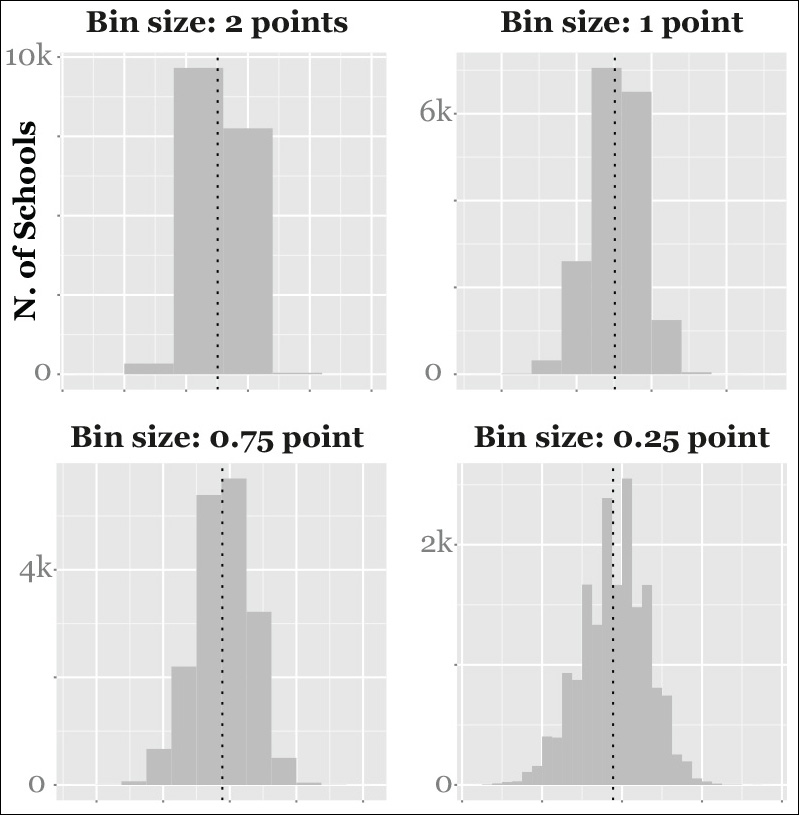
Histograms can cast light on features of the data that we may have overlooked. To begin with, we can see that most schools are close to the national mean, but just a tiny fraction of them are above the 6.0 threshold. Our distribution is almost symmetrical, and it’s close to being normal (more about this later).
Our distribution could well have been asymmetrical. For instance, income levels don’t usually follow a normal distribution but a highly skewed one, with a lot of people on the lower end of the curve and just a few individuals or families on the rightmost end of the long tail (Figure 6.7). The skew of a distribution can be a fruitful source for further exploration.9
9 Statisticians use many other measures to describe the shape of data. For instance, the peakedness of a distribution is called kurtosis, a word that, for some reason, I have always thought could be a great name for an ancient Greek hero.
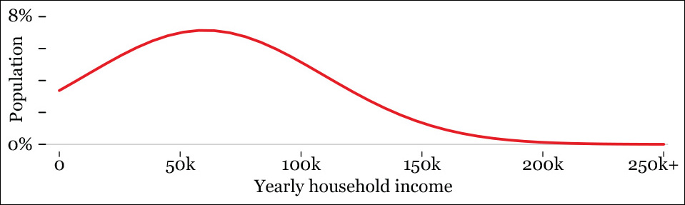
Figure 6.7 A smoothed histogram based on fictional data: the X-axis is household income, and the Y-axis is the percentage of households.
Some Fun with Ranges
Finding stories is sometimes a matter of repeatedly asking ourselves what would happen if we plot our data in a different way. We have learned about some important terms in data exploration, so let’s pause to catch our breath and play for a bit. What if we design multiple range and frequency plots, one for each of the 27 states of Brazil, and see what they tell us? Many software tools will let us do this quite quickly.
In case you’re not familiar with Brazil’s geography, I’ve designed a handy map of all 27 states and the five regions the country is divided into (Figure 6.8).
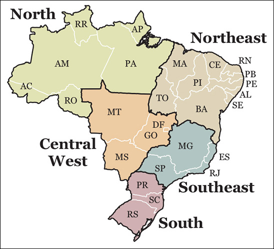
Figure 6.8 Map of Brazil. States in the north and the northeast are much poorer than those in the south and southeast.
Now, let’s roll up our sleeves and get our hands dirty.
Let’s begin with a very simple range chart (Figure 6.9) which divides our original distribution into 27, one per state in Brazil. I have arranged the states by region. Each vertical line shows the maximum, minimum, and mean score of each distribution.

Immediately, I can start writing down ideas for potential stories and infographics. There are clear differences between poor states (those in the north and the northeast) and rich states (the ones in the southeast and the south of the country).
If we focus on certain states, we’ll also notice striking facts. For instance, what’s going on in Rio de Janeiro (RJ)? It has the widest range: bad schools are among the worst overall, and its best schools are the best in the country. After consulting with experts in education, you may learn that Rio de Janeiro has the most unequal school system in Brazil, by far. We have just uncovered the evidence for that assertion.
We could go much further. Any visualization hides as much as it shows. This is certainly true of my range chart. We cannot really see any detail in it, just a crude summary of each of the 27 distributions. To understand our data well, we may want to explore them in all its glorious detail.
What if we design a chart plotting the score of each of the nearly 20,000 schools? How about a strip plot (Figure 6.10). It looks cool, I know, but don’t give me credit. Thank R, the software that I used. It took a single line of code and 10 seconds of computer processing to generate that. Then I styled it a bit in Adobe Illustrator.
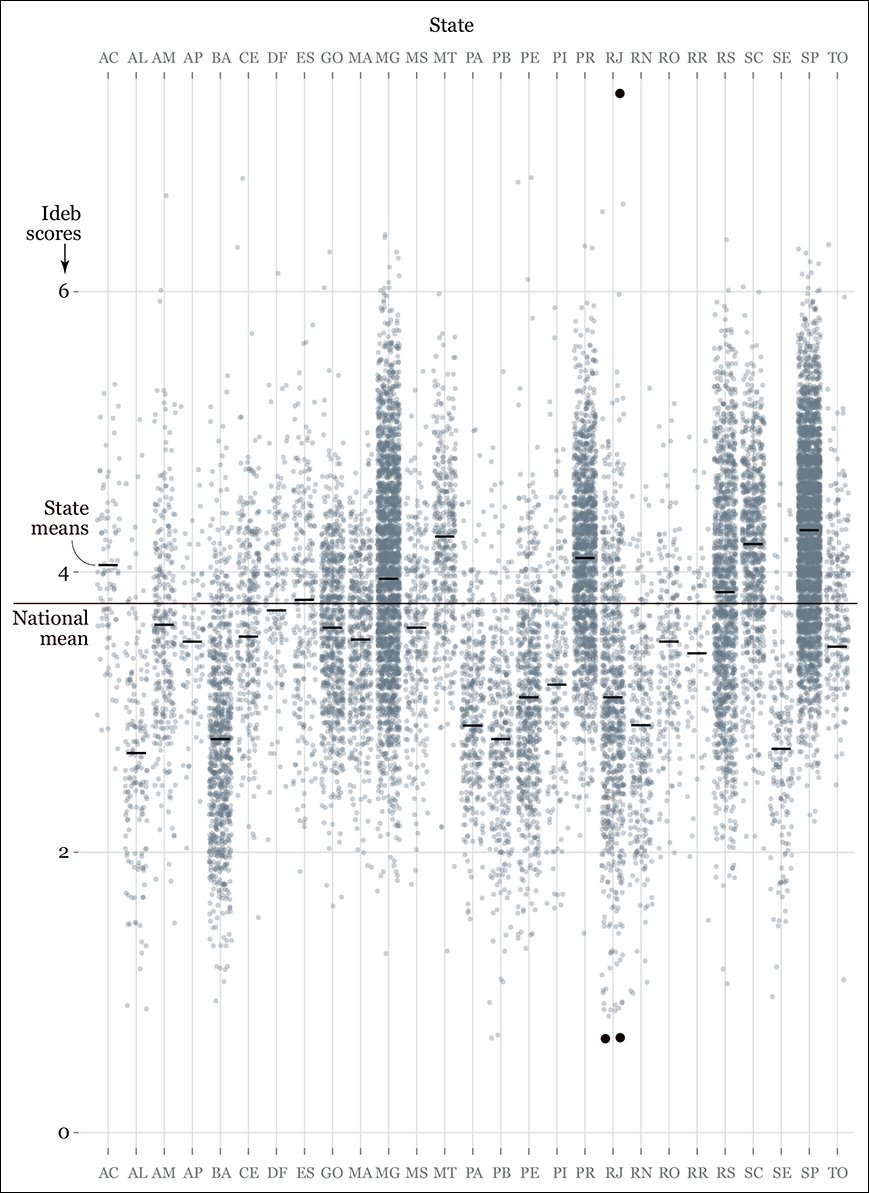
I arranged the states alphabetically because I wanted to focus on individual cases. Organizing the states in different ways (alphabetically, by region, from highest to lowest mean, and so on) could lead us to more insights, more questions to ask of our data set, and more potential stories to tell, after we corroborate them.
The black dots in the chart are the schools I highlighted for additional reporting. Perhaps I could send someone to interview the principals, or consult with the Ministry of Education about why that school at the top of the scale in Rio de Janeiro is performing so well, or what is going on with the ones at the bottom.
And this is just if I’m interested in Rio de Janeiro. I may be a citizen in the state of Ceará (CE), in which case I could zoom in on the chart to analyze its outliers. There are quite a few very visible ones. The strip plot works well when we want to compare schools at the extremes of the distribution with the norm, those schools close to the national or state means.
The histogram, the lollipop chart, and the strip plot are three ways of visualizing the spread and shape of the same distributions at different levels of detail. This is usually the best strategy: a visualization designer should never rely on a single statistic or a single chart or map when doing exploratory work.
That’s why, as you can see in Figure 6.11, I also created a histogram and a violin plot (also called a “bean plot”) for each state. These two charts may be clearer than the strip plot if our goal was to get a clear sense of frequencies, instead of visualizing each single school.
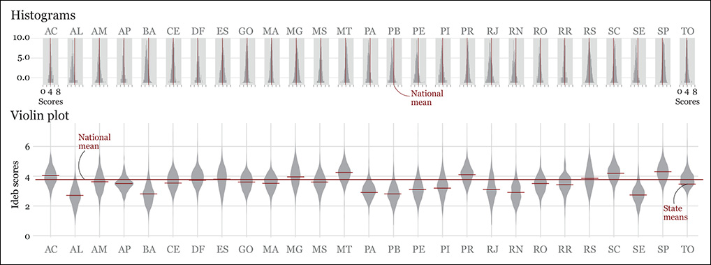
Figure 6.11 Two ways of visualizing distributions: histograms and violin plots. A violin plot is like a two-sided vertical histogram: the thickness of the color strips is proportional to counts.
Which one of these charts is better? There’s no “better.” It all depends on what we want to see. For instance, if I had to visualize the number of schools above or below the national mean on each state, I’d choose the histograms, although I’d make them much bigger. But the violin plot works great as an overview, in my opinion (besides being really pretty!). The distributions of the more equal states are very fat in the middle, as many schools are clustered around the state mean; the skinnier distributions correspond to the most unequal states, as there are few schools in the middle and more on the extremes.
Finally—and just to see what would happen—I made R generate a second strip plot of all schools in each Brazilian city. This is completely unreadable, but it certainly looks curious (Figure 6.12). It would be much more useful if we kept just a few cities and we compared them to their state or national means. Still, I have noticed some interesting facts in this mess, so I have added notes to the chart, just as a reminder to myself. They might be worth examining, who knows?
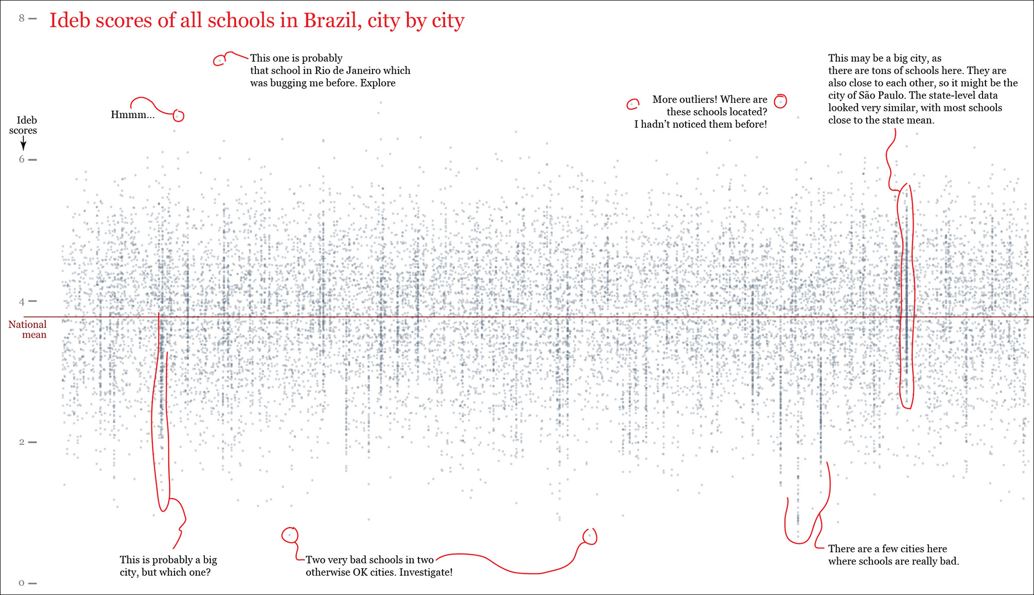
Figure 6.12 A strip plot of all schools in Brazil. Each dot represents one school, and each column of dots is a city. The annotations mimic what I do in a real project, which is to write down reminders of things that look promising in the data.
To Learn More
• Caldwell, Sally. Statistics Unplugged, 4th ed. New York, NY: Cengage Learning, 2013. If I had to recommend just one introduction to statistics book, it’d be this one.
• Hartwig, Frederick, and Brian E. Dearing. Exploratory Data Analysis. Newbury Park, CA: SAGE Publications, 1979. A concise introduction to the techniques favored by John W. Tukey.
• Wheelan, Charles. Naked Statistics: Stripping the Dread from the Data. New York, NY: W. W. Norton & Company, 2013. A pain-free overview of the core principles of statistics.