10. Catalysis and Catalytic Reactors
It isn’t that they can’t see the solution. It is that they can’t see the problem.
—G. K. Chesterton
10.1 Catalysts
Catalysts have been used by humankind for over 2000 years.1 The first observed uses of catalysts were in the making of wine, cheese, and bread. It was found that it was always necessary to add small amounts of the previous batch to make the current batch. However, it wasn’t until 1835 that Berzelius began to tie together observations of earlier chemists by suggesting that small amounts of a foreign substance could greatly affect the course of chemical reactions. This mysterious force attributed to the substance was called catalytic. In 1894, Ostwald expanded Berzelius’s explanation by stating that catalysts were substances that accelerate the rate of chemical reactions without being consumed during the reaction. During the 180 years since Berzelius’s work, catalysts have come to play a major economic role in the world market. In the United States alone, sales of process catalysts will reach over $20 billion by 2018, the major uses being in petroleum refining and in chemical production.
1 S. T. Oyama and G. A. Somorjai, J. Chem. Educ., 65, 765 (1986).
10.1.1 Definitions
A catalyst is a substance that affects the rate of a reaction but emerges from the process unchanged. A catalyst usually changes a reaction rate by promoting a different molecular path (“mechanism”) for the reaction. For example, gaseous hydrogen and oxygen are virtually inert at room temperature, but react rapidly when exposed to platinum. The reaction coordinate (cf. Chapter 3) shown in Figure 10-1 is a measure of the progress along the reaction path as H2 and O2 approach each other and pass over the activation energy barrier to form H2O. Catalysis is the occurrence, study, and use of catalysts and catalytic processes. Commercial chemical catalysts are immensely important. Approximately one-third of the material gross national product of the United States involves a catalytic process somewhere between raw material and finished product.2 The development and use of catalysts is a major part of the constant search for new ways of increasing product yield and selectivity from chemical reactions. Because a catalyst makes it possible to obtain an end product by a different pathway with a lower energy barrier, it can affect both the yield and the selectivity.
2 V. Haensel and R. L. Burwell, Jr., Sci. Am., 225(10), 46.

Catalysts can accelerate the reaction rate but cannot change the equilibrium.
Normally when we talk about a catalyst, we mean one that speeds up a reaction, although strictly speaking, a catalyst can either accelerate or slow the formation of a particular product species. A catalyst changes only the rate of a reaction; it does not affect the equilibrium.
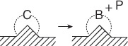
The 2007 Nobel Prize for Chemistry was awarded to Gerhard Ertl for his pioneering work on heterogeneous catalytic reactions. A heterogeneous catalytic reaction involves more than one phase; usually the catalyst is a solid and the reactants and products are in liquid or gaseous form. One example is the production of benzene, which is mostly manufactured today from the dehydrogenation of cyclohexane (obtained from the distillation of petroleum crude oil) using platinum-on-alumina as the catalyst:
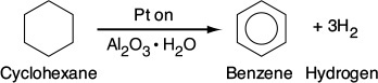
The simple and complete separation of the fluid product mixture from the solid catalyst makes heterogeneous catalysis economically attractive, especially because many catalysts are quite valuable and their reuse is demanded.
A heterogeneous catalytic reaction occurs at or very near the fluid–solid interface. The principles that govern heterogeneous catalytic reactions can be applied to both catalytic and noncatalytic fluid–solid reactions. The two other types of heterogeneous reactions involve gas–liquid and gas–liquid–solid systems. Reactions between gases and liquids are usually mass-transfer limited.
Ten grams of this catalyst possess more surface area than a U.S. football field
Catalyst types:
• Porous
• Molecular sieves
• Monolithic
• Supported
• Unsupported
Typical zeolite catalyst
High selectivity to para-xylene
10.1.2 Catalyst Properties
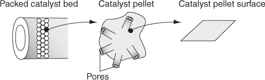
Because a catalytic reaction occurs at the fluid–solid interface, a large interfacial area is almost always essential in attaining a significant reaction rate. In many catalysts, this area is provided by an inner porous structure (i.e., the solid contains many fine pores, and the surface of these pores supplies the area needed for the high rate of reaction), see Figures 10-4(b) and 10-9. The area possessed by some porous catalysis materials is surprisingly large. A typical silica-alumina cracking catalyst has a pore volume of 0.6 cm3/g and an average pore radius of 4 nm. The corresponding surface area is 300 m2/g of these porous catalysts. Examples include the Raney nickel used in the hydrogenation of vegetable and animal oils, platinum-on-alumina used in the reforming of petroleum naphthas to obtain higher octane ratings, and promoted iron used in ammonia synthesis. Sometimes pores are so small that they will admit small molecules but prevent large ones from entering. Materials with this type of pore are called molecular sieves, and they may be derived from natural substances such as certain clays and zeolites, or they may be totally synthetic, such as some crystalline aluminosilicates (see Figure 10-2). These sieves can form the basis for quite selective catalysts; the pores can control the residence time of various molecules near the catalytically active surface to a degree that essentially allows only the desired molecules to react. One example of the high selectivity of zeolite catalysts is the formation of para-xylene from toluene and methane shown in Figure 10-2(b).3 Here, benzene and toluene enter through the zeolite pore and react on the interior surface to form a mixture of ortho-, meta-, and para-xylenes. However, the size of the pore mouth is such that only para-xylene can exit through the pore mouth, as meta- and orthoxylene with their methyl group on the side cannot fit through the pore mouth. There are interior sites that can isomerize ortho-xylene and meta-xylene to para-xylene. Hence, we have a very high selectivity to form para-xylene.
3 R. I. Masel, Chemical Kinetics and Catalysis (New York: Wiley Interscience, 2001), p. 741.

Figure 10-2 (a) Framework structures and (b) pore cross sections of two types of zeolites. (a) Faujasite-type zeolite has a three-dimensional channel system with pores at least 7.4 Å in diameter. A pore is formed by 12 oxygen atoms in a ring. (b) Schematic of reaction CH4 and C6H5CH3. (Note that the size of the pore mouth and the interior of the zeolite are not to scale.) [(a) from N. Y. Chen and T. F. Degnan, Chem. Eng. Prog., 84(2), 33 (1988). Reproduced by permission of the American Institute of Chemical Engineers. Copyright © 1988 AIChE. All rights reserved.]
In some cases a catalyst consists of minute particles of an active material dispersed over a less-active substance called a support. The active material is frequently a pure metal or metal alloy. Such catalysts are called supported catalysts, as distinguished from unsupported catalysts. Catalysts can also have small amounts of active ingredients added called promoters, which increase their activity. Examples of supported catalysts are the packed-bed catalytic converter in an automobile, the platinum-on-alumina catalyst used in petroleum reforming, and the vanadium pentoxide on silica used to oxidize sulfur dioxide in manufacturing sulfuric acid. On the other hand, platinum gauze for ammonia oxidation, promoted iron for ammonia synthesis, and the silica–alumina dehydrogenation catalyst used in butadiene manufacture typify unsupported catalysts.
10.1.3 Catalytic Gas-Solid Interactions
For the moment, let us focus our attention on gas-phase reactions catalyzed by solid surfaces. For a catalytic reaction to occur, at least one and frequently all of the reactants must become attached to the surface. This attachment is known as adsorption and takes place by two different processes: physical adsorption and chemisorption. Physical adsorption is similar to condensation. The process is exothermic, and the heat of adsorption is relatively small, being on the order of 1 to 15 kcal/mol. The forces of attraction between the gas molecules and the solid surface are weak. These van der Waals forces consist of interaction between permanent dipoles, between a permanent dipole and an induced dipole, and/or between neutral atoms and molecules. The amount of gas physically adsorbed decreases rapidly with increasing temperature, and above its critical temperature only very small amounts of a substance are physically adsorbed.
The type of adsorption that affects the rate of a chemical reaction is chemisorption. Here, the adsorbed atoms or molecules are held to the surface by valence forces of the same type as those that occur between bonded atoms in molecules. As a result, the electronic structure of the chemisorbed molecule is perturbed significantly, causing it to be extremely reactive. Interaction with the catalyst causes bonds of the adsorbed reactant to be stretched, making them easier to break.
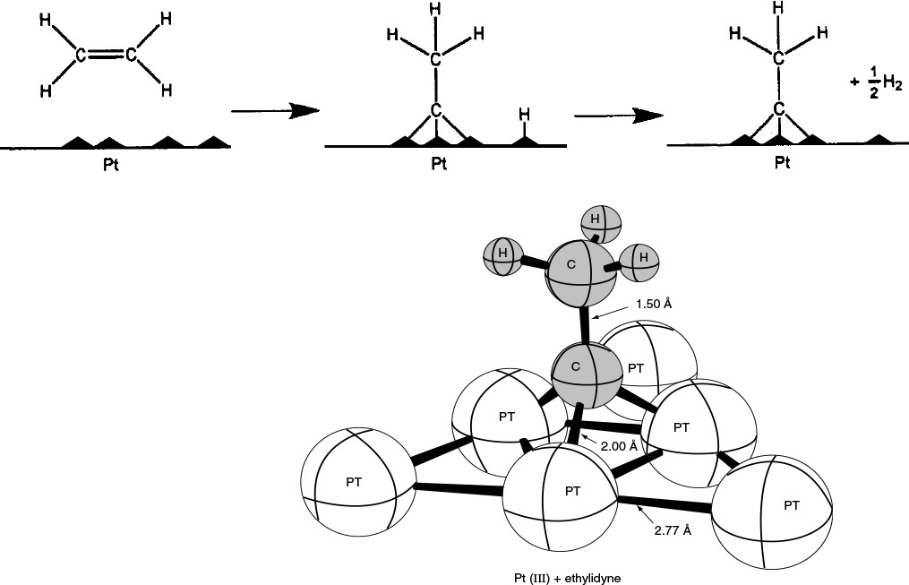
Figure 10-3 Ethylidyne chemisorbed on platinum. (Adapted from G. A. Somorjai, Introduction to Surface Chemistry and Catalysis. © 1994 John Wiley & Sons, Inc. Reprinted by permission of John Wiley & Sons, Inc. All rights reserved.)
Figure 10-3 shows the bonding from the adsorption of ethylene on a platinum surface to form chemisorbed ethylidyne. Like physical adsorption, chemisorption is an exothermic process, but the heats of adsorption are generally of the same magnitude as the heat of a chemical reaction (i.e., 40 to 400 kJ/mol). If a catalytic reaction involves chemisorption, it must be carried out within the temperature range where chemisorption of the reactants is appreciable.
In a landmark contribution to catalytic theory, Taylor suggested that a reaction is not catalyzed over the entire solid surface but only at certain active sites or centers.4 He visualized these sites as unsaturated atoms in the solids that resulted from surface irregularities, dislocations, edges of crystals, and cracks along grain boundaries. Other investigators have taken exception to this definition, pointing out that other properties of the solid surface are also important. The active sites can also be thought of as places where highly reactive intermediates (i.e., chemisorbed species) are stabilized long enough to react. This stabilization of a reactive intermediate is key in the design of any catalyst. Consequently, for our purposes we will define an active site as a point on the catalyst surface that can form strong chemical bonds with an adsorbed atom or molecule.
4 H. S. Taylor, Proc. R. Soc. London, A108, 105 (1928).
Chemisorption on active sites is what catalyzes the reaction.
One parameter used to quantify the activity of a catalyst is the turnover frequency (TOF), f. It is the number of molecules reacting per active site per second at the conditions of the experiment. When a metal catalyst such as platinum is deposited on a support, the metal atoms are considered active sites. The TOFs for a number of reactions are shown in Professional Reference Shelf R10.1. The dispersion, D, of the catalyst is the fraction of the metal atoms deposited on a catalyst that are on the surface.
10.1.4 Classification of Catalysts
One common way to classify catalysts is in terms of the type of reaction they catalyze.
Table 10-1 gives a list of representative reactions and their corresponding catalysts. Further discussion of each of these reaction classes and the materials that catalyze them can be found on the CRE Web site’s Professional Reference Shelf R10.1.

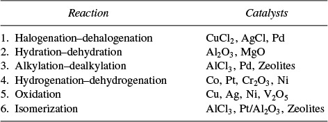
If, for example, we were to form styrene from an equimolar mixture of ethylene and benzene, we could first carry out an alkylation reaction to form ethyl benzene, which is then dehydrogenated to form styrene. We need both an alkylation catalyst and a dehydrogenation catalyst:
10.2 Steps in a Catalytic Reaction
A photograph of different types and sizes of catalysts is shown in Figure 10-4a. A schematic diagram of a tubular reactor packed with catalytic pellets is shown in Figure 10-4b. The overall process by which heterogeneous catalytic reactions proceed can be broken down into the sequence of individual steps shown in Table 10-2 and pictured in Figure 10-5 for an isomerization reaction.
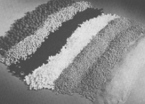
Figure 10-4a Catalyst particles of different shapes (spheres, cylinders) and sizes (0.1 cm to 1 cm). (Photo courtesy of the Engelhard Corporation.)
Each step in Table 10-2 is shown schematically in Figure 10-5.
A reaction takes place on the surface, but the species involved in the reaction must get to and from the surface.
The overall rate of reaction is limited by the rate of the slowest step in the sequence. When the diffusion steps (1, 2, 6, and 7 in Table 10-2) are very fast compared with the surface reaction-rate steps (3, 4, and 5), the concentrations in the immediate vicinity of the active sites are indistinguishable from those in the bulk fluid. In this situation, the transport or diffusion steps do not affect the overall rate of the reaction. In other situations, if the reaction steps are very fast compared with the diffusion steps, mass transport does affect the reaction rate. In systems where diffusion from the bulk gas or liquid to the external catalyst surface or to the mouths of catalyst pores affects the rate, i.e., steps 1 and 7, changing the flow conditions past the catalyst should change the overall reaction rate (see Chapter 14). Once inside the porous catalysts, on the other hand, diffusion within the catalyst pores, i.e., steps 2 and 6, may limit the rate of reaction and, as a result, the overall rate will be unaffected by external flow conditions even though diffusion affects the overall reaction rate (see Chapter 15).
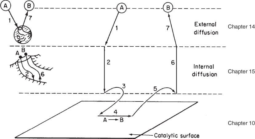
1. Mass transfer (diffusion) of the reactant(s) (e.g., species A) from the bulk fluid to the external surface of the catalyst pellet
2. Diffusion of the reactant from the pore mouth through the catalyst pores to the immediate vicinity of the internal catalytic surface
3. Adsorption of reactant A onto the catalyst surface
4. Reaction on the surface of the catalyst (e.g., ![]() )
)
5. Desorption of the products (e.g., B) from the surface
6. Diffusion of the products from the interior of the pellet to the pore mouth at the external surface
7. Mass transfer of the products from the external pellet surface to the bulk fluid
TABLE 10-2 STEPS IN A CATALYTIC REACTION
There are many variations of the situation described in Table 10-2. Sometimes, of course, two reactants are necessary for a reaction to occur, and both of these may undergo the steps listed above. Other reactions between two substances may have only one of them adsorbed.
In this chapter we focus on:
3. Adsorption
4. Surface reaction
5. Desorption
With this introduction, we are ready to treat individually the steps involved in catalytic reactions. In this chapter, only steps 3, 4, and 5—i.e., adsorption, surface reaction, and desorption—are considered as we assume that the diffusion steps (1, 2, 6, and 7) are very fast so that the overall reaction rate is not affected by mass transfer in any fashion. Further treatment of the effects involving diffusion limitations is provided in Chapters 14 and 15.
Where Are We Heading?† As we saw in Chapter 7, one of the tasks of a chemical reaction engineer is to analyze rate data and to develop a rate law that can be used in reactor design. Rate laws in heterogeneous catalysis seldom follow power-law models and hence are inherently more difficult to formulate from the data. To develop an in-depth understanding and insight as to how the rate laws are formed from heterogeneous catalytic data, we are going to proceed in somewhat of a reverse manner than what is normally done in industry when one is asked to develop a rate law. That is, we will postulate catalytic mechanisms and then derive rate laws for the various mechanisms. The mechanism will typically have an adsorption step, a surface reaction step, and a desorption step, one of which is usually rate-limiting. Suggesting mechanisms and rate-limiting steps is not the first thing we normally do when presented with data. However, by deriving equations for different mechanisms, we will observe the various forms of the rate law one can have in heterogeneous catalysis. Knowing the different forms that catalytic rate equations can take, it will be easier to view the trends in the data and deduce the appropriate rate law. This deduction is usually what is done first in industry before a mechanism is proposed. Knowing the form of the rate law, one can then numerically evaluate the rate-law parameters and postulate a reaction mechanism and rate-limiting step that are consistent with the rate data. Finally, we use the rate law to design catalytic reactors. This procedure is shown in Figure 10-6. The dashed lines represent feedback to obtain new data in specific regions (e.g., concentrations, temperature) to evaluate the rate-law parameters more precisely or to differentiate between reaction mechanisms.
† “If you don’t know where you are going, you’ll probably wind up someplace else.” Yogi Berra
An algorithm

We will discuss each of the steps shown in Figure 10-5 and Table 10-2. As mentioned earlier, this chapter focuses on Steps 3, 4, and 5 (the adsorption, surface reaction and desorption steps) by assuming that Steps 1, 2, 6, and 7 are very rapid. Consequently, to understand when this assumption is valid, we shall give a quick overview of Steps 1, 2, 6, and 7. These steps involve diffusion of the reactants to and within the catalyst pellet. While these diffusion steps are covered in detail in Chapters 14 and 15, it is worthwhile to give a brief description of these two mass-transfer steps to better understand the entire sequence of steps. If you have had the core course in Mass Transfer or Transport Phenomena you can skip Sections 10.2.1 and 10.2.2, and go directly to Section 10.2.3.
Chance Card: Do not pass go proceed directly to Section 10.2.3.

10.2.1 Step 1 Overview: Diffusion from the Bulk to the External Surface of the Catalyst
For the moment let’s assume that the transport of A from the bulk fluid to the external surface of the catalyst is the slowest step in the sequence. We lump all the resistance to transfer from the bulk fluid to the surface in the mass-transfer boundary layer surrounding the pellet. In this step the reactant A, which is at a bulk concentration CAb must travel (diffuse) through the boundary layer of thickness δ to the external surface of the pellet where the concentration is CAs, as shown in Figure 10-7. The rate of transfer (and hence rate of reaction, ![]() ) for this slowest step is
) for this slowest step is
Rate = kC (CAb – CAs)
External and internal mass transfer in catalysis are covered in detail in Chapters 14 and 15.
where the mass-transfer coefficient, kC, is a function of the hydrodynamic conditions, namely the fluid velocity, U, and the particle diameter, Dp.
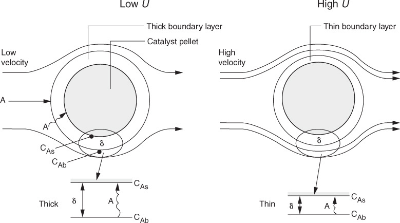
Figure 10-7 Diffusion through the external boundary layer (also see Figure 14-3).
External mass transfer
“The thick and thin of it.”
As we see (Chapter 14), the mass-transfer coefficient is inversely proportional to the boundary layer thickness, δ, and directly proportional to the diffusion coefficient (i.e., the diffusivity DAB).
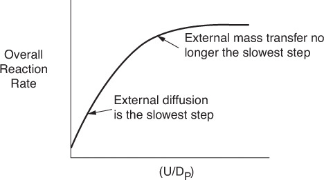
At low velocities of fluid flow over the pellet, the boundary layer across which A and B must diffuse is thick, and it takes a long time for A to travel to the surface, resulting in a small mass-transfer coefficient kC. As a result, mass transfer across the boundary layer is slow and limits the rate of the overall reaction. As the velocity over the pellet is increased, the boundary layer becomes thinner and the mass-transfer rate is increased. At very high velocities, the boundary layer thickness, δ, is so small it no longer offers any resistance to the diffusion across the boundary layer. As a result, external mass transfer no longer limits the rate of reaction. This external resistance also decreases as the particle size is decreased. As the fluid velocity increases and/or the particle diameter decreases, the mass-transfer coefficient increases until a plateau is reached, as shown in Figure 10-8. On this plateau, CAb ≈ CAs, and one of the other steps in the sequence, i.e., Steps 2 through 6, is the slowest step and limits the overall reaction rate. Further details on external mass transfer are discussed in Chapter 14.
10.2.2 Step 2 Overview: Internal Diffusion
Now consider that we are operating at a fluid velocity where external diffusion is no longer the rate-limiting step and that internal diffusion is the slowest step. In Step 2 the reactant A diffuses from the external pellet surface at a concentration CAs into the pellet interior, where the concentration is CA. As A diffuses into the interior of the pellet, it reacts with catalyst deposited on the sides of the catalyst pellet’s pore walls.
For large pellets, it takes a long time for the reactant A to diffuse into the interior, compared to the time that it takes for the reaction to occur on the interior pore surface. Under these circumstances, the reactant is only consumed near the exterior surface of the pellet and the catalyst near the center of the pellet is wasted catalyst. On the other hand, for very small pellets it takes very little time to diffuse into and out of the pellet interior and, as a result, internal diffusion no longer limits the rate of reaction. When internal mass transfer no longer limits the rate of reaction, the rate law can be expressed as
Rate = kr CAs
where CAs is the concentration at the external pellet surface and kr is an overall rate constant, which is a function of particle size. The overall rate constant, kr, increases as the pellet diameter decreases. In Chapter 15, we show that Figure 15-5 can be combined with Equation (15-34) to arrive at the plot of kr as a function of DP, shown in Figure 10-9(b).
We see in Figure 10-9 that at small particle sizes, internal diffusion is no longer the slow step and that the surface reaction sequence of adsorption, surface reaction, and desorption (Steps 3, 4, and 5 in Figure 10-5) limit the overall rate of reaction. Consider now one more important point about internal diffusion and surface reaction. These steps (2 through 6) are not at all affected by flow conditions external to the pellet.
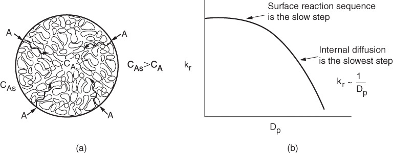
Figure 10-9 Effect of particle size on the overall reaction-rate constant. (a) Branching of a single pore with deposited metal; (b) decrease in rate constant with increasing particle diameter. (See the CRE Web site, Chapter 12.)
Internal mass transfer
In the material that follows, we are going to choose our pellet size and external fluid velocity such that neither external diffusion nor internal diffusion is limiting as discussed in Chapters 14 and 15. Instead, we assume that either Step 3 (adsorption), Step 4 (surface reaction), or Step 5 (desorption), or a combination of these steps, limits the overall rate of reaction.
10.2.3 Adsorption Isotherms
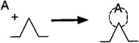
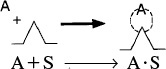
Because chemisorption is usually a necessary part of a catalytic process, we shall discuss it before treating catalytic reaction rates. The letter S will represent an active site; alone, it will denote a vacant site, with no atom, molecule, or complex adsorbed on it. The combination of S with another letter (e.g., A ·S) will mean that one unit of species A will be chemically adsorbed on the site S. Species A can be an atom, molecule, or some other atomic combination, depending on the circumstances. Consequently, the adsorption of A on a site S is represented by
The total molar concentration of active sites per unit mass of catalyst is equal to the number of active sites per unit mass divided by Avogadro’s number and will be labeled Ct (mol/g-cat). The molar concentration of vacant sites, Cv (mol/g-cat), is the number of vacant sites per unit mass of catalyst divided by Avogadro’s number. In the absence of catalyst deactivation, we assume that the total concentration of active sites, Ct, remains constant. Some further definitions include
Pi = partial pressure of species i in the gas phase, (atm or kPa)
Ci·S = surface concentration of sites occupied by species i, (mol/g-cat)
A conceptual model depicting species A and B adsorbed on two different sites is shown in Figure 10-10.
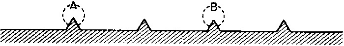
For the system shown in Figure 10-10, the total concentration of sites is
Site balance
This equation is referred to as a site balance. A typical value for the total concentration of sites could be the order of 1022 sites/g-cat.
Now consider the adsorption of a nonreacting gas onto the surface of a catalyst. Adsorption data are frequently reported in the form of adsorption isotherms. Isotherms portray the amount of a gas adsorbed on a solid at different pressures at a given temperature.
Postulate models; then see which one(s) fit(s) the data.
First, an adsorption mechanism is proposed, and then the isotherm (see Figure 10-11, page 413) obtained from the mechanism is compared with the experimental data. If the isotherm predicted by the model agrees with the experimental data, the model may reasonably describe what is occurring physically in the real system. If the predicted curve does not agree with the experimental data, the model fails to match the physical situation in at least one important characteristic and perhaps more.
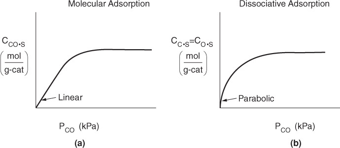
We will consider two types of adsorption: molecular adsorption and dissociative adsorption. To illustrate the difference between molecular adsorption and dissociative adsorption, we will postulate two models for the adsorption of carbon monoxide on metal surfaces. In the molecular adsorption model, CO is adsorbed as molecules, CO,
as is the case on nickel
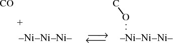
Two models:
1. Adsorption as CO
2. Adsorption as C and O
In the dissociative adsorption model, carbon monoxide is adsorbed as oxygen and carbon atoms instead of molecular CO
as is the case on iron5
5 R. I. Masel, Principles of Adsorption and Reaction on Solid Surfaces (New York: Wiley, 1996).

The former is called molecular or nondissociated adsorption (e.g., CO) and the latter is called dissociative adsorption (e.g., C and O). Whether a molecule adsorbs nondissociatively or dissociatively depends on the surface.
The adsorption of carbon monoxide molecules will be considered first. Because the carbon monoxide does not react further after being adsorbed, we need only to consider the adsorption process:
Molecular Adsorption
In obtaining a rate law for the rate of adsorption, the reaction in Equation (10-2) can be treated as an elementary reaction. The rate of attachment of the carbon monoxide molecules to the active site on the surface is proportional to the number of collisions that these molecules make with a surface active site per second. In other words, a specific fraction of the molecules that strike the surface become adsorbed. The collision rate is, in turn, directly proportional to the carbon monoxide partial pressure, PCO. Because carbon monoxide molecules adsorb only on vacant sites and not on sites already occupied by other carbon monoxide molecules, the rate of attachment is also directly proportional to the concentration of vacant sites, Cv. Combining these two facts means that the rate of attachment of carbon monoxide molecules to the surface is directly proportional to the product of the partial pressure of CO and the concentration of vacant sites; that is,
Rate of attachment = kAPCOCv
The rate of detachment of molecules from the surface can be a first-order process; that is, the detachment of carbon monoxide molecules from the surface is usually directly proportional to the concentration of sites occupied by the adsorbed molecules (e.g., CCO ·S):
Rate of detachment = k–ACCO·S
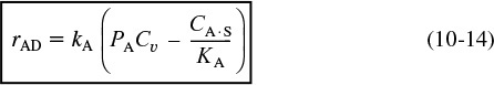
The net rate of adsorption is equal to the rate of molecular attachment to the surface minus the rate of detachment from the surface. If kA and k–A are the constants of proportionality for the attachment and detachment processes, then
The ratio KA = kA/k–A is the adsorption equilibrium constant. Using KA to rearrange Equation (10-3) gives
Adsorption

The adsorption rate constant, kA, for molecular adsorption is virtually independent of temperature, while the desorption constant, k–A, increases exponentially with increasing temperature. Consequently, the equilibrium adsorption constant KA decreases exponentially with increasing temperature.
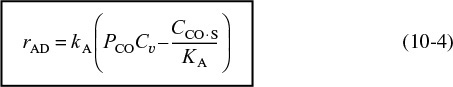
Because carbon monoxide is the only material adsorbed on the catalyst, the site balance gives
At equilibrium, the net rate of adsorption equals zero, i.e., rAD ≡ 0. Setting the left-hand side of Equation (10-4) equal to zero and solving for the concentration of CO adsorbed on the surface, we get
Using Equation (10-5) to give Cv in terms of CCO ·S and the total number of sites Ct, we can solve for the equilibrium value of CCO·S in terms of constants and the pressure of carbon monoxide
CCO · S = KA Cv PCO = KAPCO(Ct – CCO · S)
Rearranging gives us
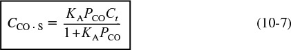

This equation thus gives the equilibrium concentration of carbon monoxide adsorbed on the surface, CCO ·S, as a function of the partial pressure of carbon monoxide, and is an equation for the adsorption isotherm. This particular type of isotherm equation is called a Langmuir isotherm.6 Figure 10-11(a) shows the Langmuir isotherm for the amount of CO adsorbed per unit mass of catalyst as a function of the partial pressure of CO. For the case of dissociative adsorption, Equation (10-11), Figure 10-11(b), shows the concentration of the atoms C and O adsorbed per unit mass of catalyst.
6 Named after Irving Langmuir (1881–1957), who first proposed it. He received the Nobel Prize in 1932 for his discoveries in surface chemistry.
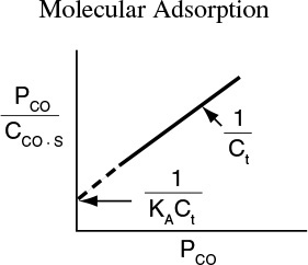
One method of checking whether a model (e.g., molecular adsorption versus dissociative adsorption) predicts the behavior of the experimental data is to linearize the model’s equation and then plot the indicated variables against one another. For example, the molecular adsorption isotherm, Equation (10-7), may be arranged in the form
and the linearity of a plot of PCO/CCO ·S as a function of PCO will determine if the data conform to molecular adsorption, i.e., a Langmuir single-site isotherm.
Next, we derive the isotherm for carbon monoxide disassociating into separate atoms as it adsorbs on the surface, i.e.,
Dissociative adsorption
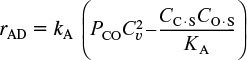
When the carbon monoxide molecule dissociates upon adsorption, it is referred to as the dissociative adsorption of carbon monoxide. As in the case of molecular adsorption, the rate of adsorption is proportional to the pressure of carbon monoxide in the system because this rate is governed by the number of gaseous collisions with the surface. For a molecule to dissociate as it adsorbs, however, two adjacent vacant active sites are required, rather than the single site needed when a substance adsorbs in its molecular form. The probability of two vacant sites occurring adjacent to one another is proportional to the square of the concentration of vacant sites. These two observations mean that the rate of adsorption is proportional to the product of the carbon monoxide partial pressure and the square of the vacant-site concentration, ![]() .
.
For desorption to occur, two occupied sites must be adjacent, meaning that the rate of desorption is proportional to the product of the occupied-site concentration, (C · S) × (O · S). The net rate of adsorption can then be expressed as
Factoring out kA, the equation for dissociative adsorption is
where
Rate of dissociative adsorption
For dissociative adsorption, both kA and k–A increase exponentially with increasing temperature, while the adsorption equilibrium constant KA decreases with increasing temperature.
At equilibrium, rAD ≡ 0, and
For CC·S = CO·S
Substituting for CC·S and CO·S in a site balance equation (10-1),

Solving for Cv
Cv = Ct/(1+2(KCOPCO)1/2)
This value may be substituted into Equation (10-10) to give an expression that can be solved for the equilibrium value of CO·S. The resulting equation for the isotherm shown in Figure 10-11(b) is

Langmuir isotherm for carbon monoxide dissociative adsorption as atomic carbon and oxygen
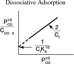
Taking the inverse of both sides of the equation, then multiplying through by (PCO)1/2, yields
If dissociative adsorption is the correct model, a plot of ![]() ver sus
ver sus ![]() should be linear with slope (2/Ct).
should be linear with slope (2/Ct).
When more than one substance is present, the adsorption isotherm equations are somewhat more complex. The principles are the same, though, and the isotherm equations are easily derived. It is left as an exercise to show that the adsorption isotherm of A in the presence of another adsorbate B is given by the relationship

When the adsorption of both A and B are first-order processes, the desorptions are also first order, and both A and B are adsorbed as molecules. The derivations of other Langmuir isotherms are relatively easy.
In obtaining the Langmuir isotherm equations, several aspects of the adsorption system were presupposed in the derivations. The most important of these, and the one that has been subject to the greatest doubt, is that a uniform surface is assumed. In other words, any active site has the same attraction for an impinging molecule as does any other active site. Isotherms different from the Langmuir isotherm, such as the Freundlich isotherm, may be derived based on various assumptions concerning the adsorption system, including different types of nonuniform surfaces.
Note assumptions in the model and check their validity.
is given by
Surface reaction models
After a reactant has been adsorbed onto the surface, i.e., A · S, it is capable of reacting in a number of ways to form the reaction product. Three of these ways are:
1. Single site. The surface reaction may be a single-site mechanism in which only the site on which the reactant is adsorbed is involved in the reaction. For example, an adsorbed molecule of A may isomerize (or perhaps decompose) directly on the site to which it is attached, such as

The pentane isomerization can be written in generic form as

Each step in the reaction mechanism is elementary, so the surface reaction rate law is

Single Site ![]()
Ks = (dimensionless)
where KS is the surface-reaction equilibrium constant KS = kS/k–S
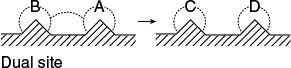
2. Dual site. The surface reaction may be a dual-site mechanism in which the adsorbed reactant interacts with another site (either unoccupied or occupied) to form the product.
First type of dual-site mechanism

For example, adsorbed A may react with an adjacent vacant site to yield a vacant site and a site on which the product is adsorbed, or as in the case of the dehydration of butanol, the products may adsorb on two adjacent sites.

C4H9OH · S + S → C4Hg · S + H2O · S

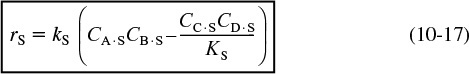
For the generic reaction
the corresponding surface-reaction rate law is

Dual Site
A second dual-site mechanism is the reaction between two adsorbed species, such as the reaction of CO with O.
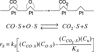
For the generic reaction
the corresponding surface-reaction rate law is
A third dual-site mechanism is the reaction of two species adsorbed on different types of sites S and S’, such as the reaction of CO with O.
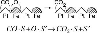
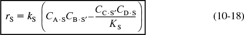
For the generic reaction

the corresponding surface-reaction rate law is
Reactions involving either single- or dual-site mechanisms, which were described earlier, are sometimes referred to as following Langmuir–Hinshelwood kinetics.
Langmuir–Hinshelwood kinetics
3. Eley–Rideal. A third mechanism is the reaction between an adsorbed molecule and a molecule in the gas phase, such as the reaction of propylene and benzene (cf. the reverse reaction in Figure 10-13)
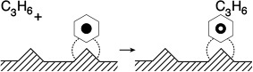
For the generic reaction
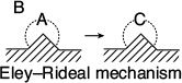
the corresponding surface-reaction rate law is
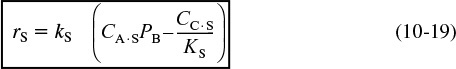
This type of mechanism is referred to as an Eley–Rideal mechanism.
10.2.5 Desorption
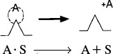
In each of the preceding cases, the products of the surface reaction adsorbed on the surface are subsequently desorbed into the gas phase. For the desorption of a species (e.g., C)

the rate of desorption of C is
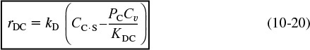
where KDC is the desorption equilibrium constant with units of atm. Now let’s look at the above adsorption from right to left. We note that the desorption step for C is just the reverse of the adsorption step. Consequently, the rate of desorption of C, rDC, is just opposite in sign to the rate of adsorption of C, rADC
rDC = –rADC
In addition, we see that the desorption equilibrium constant KDC is just the reciprocal of the adsorption equilibrium constant for C, KC

in which case the rate of desorption of C can be written
In the material that follows, the form of the equation for the desorption step that we will use to develop our rate laws will be similar to Equation (10-21).
10.2.6 The Rate-Limiting Step
When heterogeneous reactions are carried out at steady state, the rates of each of the three reaction steps in series (adsorption, surface reaction, and desorption) are equal to one another
However, one particular step in the series is usually found to be ratelimiting or rate-controlling. That is, if we could make that particular step go faster, the entire reaction would proceed at an accelerated rate. Consider the analogy to the electrical circuit shown in Figure 10-12. A given concentration of reactants is analogous to a given driving force or electromotive force (EMF). The current I (with units of Coulombs/s) is analogous to the rate of

reaction, ![]() (mol/s · g-cat), and a resistance Ri is associated with each step in the series. Because the resistances are in series, the total resistance Rtot is just the sum of the individual resistances, for adsorption (RAD), surface reaction (RS), and desorption (RD). The current, I, for a given voltage, E, is
(mol/s · g-cat), and a resistance Ri is associated with each step in the series. Because the resistances are in series, the total resistance Rtot is just the sum of the individual resistances, for adsorption (RAD), surface reaction (RS), and desorption (RD). The current, I, for a given voltage, E, is
Because we observe only the total resistance, Rtot, it is our task to find which resistance is much larger (say, 100 Ω) than the other two resistances (say, 0.1 Ω). Thus, if we could lower the largest resistance, the current I (i.e., ![]() ), would be larger for a given voltage, E. Analogously, we want to know which step in the adsorption–reaction–desorption series is limiting the overall rate of reaction.
), would be larger for a given voltage, E. Analogously, we want to know which step in the adsorption–reaction–desorption series is limiting the overall rate of reaction.
The concept of a rate-limiting step
Who is slowing us down?
The approach in determining catalytic and heterogeneous mechanisms is usually termed the Langmuir–Hinshelwood approach, since it is derived from ideas proposed by Hinshelwood based on Langmuir’s principles for adsorption.7 The Langmuir–Hinshelwood approach was popularized by Hougen and Watson and occasionally includes their names.8 It consists of first assuming a sequence of steps in the reaction. In writing this sequence, one must choose among such mechanisms as molecular or atomic adsorption, and single- or dual-site reaction. Next, rate laws are written for the individual steps as shown in the preceding section, assuming that all steps are reversible. Finally, a rate-limiting step is postulated, and steps that are not rate-limiting are used to eliminate all coverage-dependent terms. The most questionable assumption in using this technique to obtain a rate law is the hypothesis that the activity of the surface is essentially uniform as far as the various steps in the reaction are concerned.
7 C. N. Hinshelwood, The Kinetics of Chemical Change (Oxford: Clarendon Press, 1940).
8 O. A. Hougen and K. M. Watson, Ind. Eng. Chem., 35, 529 (1943).
Industrial Example of Adsorption-Limited Reaction
An example of an adsorption-limited reaction is the synthesis of ammonia from hydrogen and nitrogen
over an iron catalyst that proceeds by the following mechanism:9
9 From the literature cited in G. A. Somorjai, Introduction to Surface Chemistry and Catalysis (New York: Wiley, 1994), p. 482.
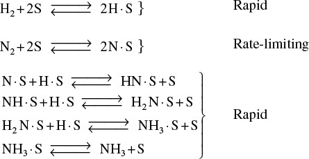
Dissociative adsorption of N2 is rate-limiting
The rate-limiting step is believed to be the adsorption of the N2 molecule as an N atom.
Industrial Example of Surface-Limited Reaction
An example of a surface-limited reaction is the reaction of two noxious automobile exhaust products, CO and NO
carried out over a copper catalyst to form environmentally acceptable products, N2 and CO2
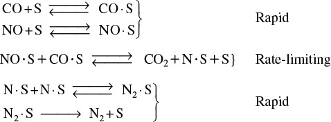
Surface reaction is rate-limiting
Analysis of the rate law suggests that CO2 and N2 are weakly adsorbed, i.e., have infinitesimally small adsorption constants (see Problem P10-9B).
10.3 Synthesizing a Rate Law, Mechanism, and Rate-Limiting Step
We now wish to develop rate laws for catalytic reactions that are not diffusion-limited. In developing the procedure to obtain a mechanism, a rate-limiting step, and a rate law consistent with experimental observation, we shall discuss a particular catalytic reaction, the decomposition of cumene to form benzene and propylene. The overall reaction is
A conceptual model depicting the sequence of steps in this platinum-catalyzed reaction is shown in Figure 10-13. Figure 10-13 is only a schematic representation of the adsorption of cumene; a more realistic model is the formation of a complex of the π orbitals of benzene with the catalytic surface, as shown in Figure 10-14.
• Adsorption
• Surface reaction
• Desorption
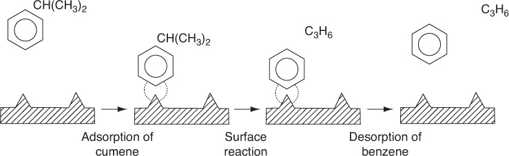

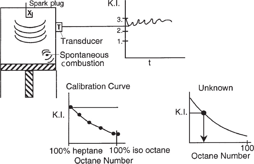
The nomenclature in Table 10-3 will be used to denote the various species in this reaction: C = cumene, B = benzene, and P = propylene. The reaction sequence for this decomposition is shown in Table 10-3.

These three steps represent the mechanism for cumene decomposition.
Equations (10-22) through (10-24) represent the mechanism proposed for this reaction.
When writing rate laws for these steps, we treat each step as an elementary reaction; the only difference is that the species concentrations in the gas phase are replaced by their respective partial pressures
Ideal gas law PC = CCRT
There is no theoretical reason for this replacement of the concentration, CC, with the partial pressure, PC; it is just the convention initiated in the 1930s and used ever since. Fortunately, PC can be calculated easily and directly from CC using the ideal gas law (i.e., PC = CCRT).
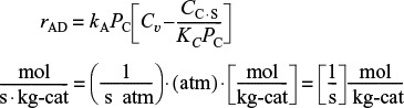
The rate expression for the adsorption of cumene as given in Equation (10-22) is
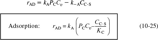
If rAD has units of (mol/g-cat·s) and CC·S has units of (mol cumene adsorbed/g-cat), then typical units of kA, k–A, and KC would be

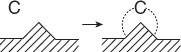
The rate law for the surface-reaction step producing adsorbed benzene and propylene in the gas phase
is
rS = kS CC·S – k–SPPCB·S
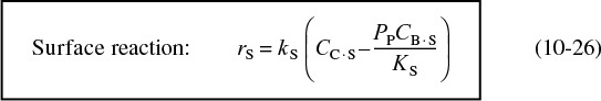
with the surface reaction equilibrium constant being
Typical units for kS and KS are s–1 and kPa, respectively.
Propylene is not adsorbed on the surface. Consequently, its concentration on the surface is zero.
CP·S = 0
The rate of benzene desorption [see Equation (10-24)] is


Typical units of kD and KDB are s–1 and kPa, respectively. By viewing the desorption of benzene
from right to left, we see that desorption is just the reverse of the adsorption of benzene. Consequently, as mentioned earlier, it is easily shown that the benzene adsorption equilibrium constant KB is just the reciprocal of the benzene desorption constant KDB
and Equation (10-28) can be written as
Because there is no accumulation of reacting species on the surface, the rates of each step in the sequence are all equal as discussed in Figure 10-12:
For the mechanism postulated in the sequence given by Equations (10-22) through (10-24), we wish to determine which step is rate-limiting. We first assume one of the steps to be rate-limiting (rate-controlling) and then formulate the reaction-rate law in terms of the partial pressures of the species present. From this expression we can determine the variation of the initial reaction rate with the initial partial pressures and the initial total pressure. If the predicted rate varies with pressure in the same manner as the rate observed experimentally, the implication is that the assumed mechanism and rate-limiting step are correct.
We will first start our development of the rate laws with the assumption that the adsorption step is rate-limiting and derive the rate law, and then proceed to assume that each of the other two steps’ surface reaction and desorption limit the overall rate and then derive the rate law for each of these other two limiting cases.
10.3.1 Is the Adsorption of Cumene Rate-Limiting?
To answer this question we shall assume that the adsorption of cumene is indeed rate-limiting, derive the corresponding rate law, and then check to see if it is consistent with experimental observation. By postulating that this (or any other) step is rate-limiting, we are assuming that the reaction-rate constant of this step (in this case kA) is small with respect to the specific rates of the other steps (in this case kS and kD).10 The rate of adsorption is
10 Strictly speaking, one should compare the product kA PC with kS and kD.
Dividing rAD by kAPC, we note ![]() . The reason we do this is that in order to compare terms, the ratios
. The reason we do this is that in order to compare terms, the ratios ![]() , and
, and ![]() must all have the same units
must all have the same units ![]() . Luckily for us, the end result is the same, however.
. Luckily for us, the end result is the same, however.

Need to express Cv and CC·S in terms of PC, PB, and PP
Because we cannot measure either Cv or CC·S, we must replace these variables in the rate law with measurable quantities for the equation to be meaningful.
For steady-state operation we have
For adsorption-limited reactions, kA is very small and kS and kD are very, very large by comparison. Consequently, the ratios rS/kS and rD/kD are very small (approximately zero), whereas the ratio rAD/kA is relatively large.
The surface reaction-rate law is

Again, for adsorption-limited reactions, the surface-specific reaction rate kS is large by comparison, and we can set
and solve Equation (10-31) for CC·S
To be able to express CC·S solely in terms of the partial pressures of the species present, we must evaluate CB·S. The rate of desorption of benzene is
However, for adsorption-limited reactions, kD is large by comparison, and we can set
Using ![]() to find CB·S and CC·S in terms of partial pressures
to find CB·S and CC·S in terms of partial pressures
and then solve Equation (10-29) for CB·S
After combining Equations (10-33) and (10-35), we have
Replacing CC·S in the rate equation by Equation (10-36) and then factoring Cv, we obtain

Let’s look at how the thermodynamic constant pressure equilibrium constant, KP, found its way into Equation (10-37) and how we can find its value for any reaction. First we observe that at equilibrium rAD = 0, Equation (10-37) rearranges to
We also know from thermodynamics (Appendix C) that for the reaction
also at equilibrium (![]() ), we have the following relationship for partial pressure equilibrium constant KP
), we have the following relationship for partial pressure equilibrium constant KP
Consequently, the following relationship must hold

The equilibrium constant can be determined from thermodynamic data and is related to the change in the Gibbs free energy, ΔG°, by the equation (see Appendix C)
where R is the ideal gas constant and T is the absolute temperature.
The concentration of vacant sites, Cv, can now be eliminated from Equation (10-37) by utilizing the site balance to give the total concentration of sites, Ct, which is assumed constant11
11 Some (I won’t mention any names) prefer to write the surface reaction rate in terms of the fraction of the surface of sites covered (i.e., fA) rather than the number of sites CA · S covered, the difference being the multiplication factor of the total site concentration, Ct. In any event, the final form of the rate law is the same because Ct, KA, kS, and so on, are all lumped into the reaction-rate constant, k.
Because cumene and benzene are adsorbed on the surface, the concentration of occupied sites is (CC·S + CB·S), and the total concentration of sites is
Site balance
Substituting Equations (10-35) and (10-36) into Equation (10-40), we have
Solving for Cv, we have
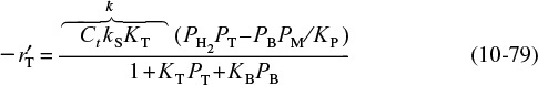
Combining Equations (10-41) and (10-37), we find that the rate law for the catalytic decomposition of cumene, assuming that the adsorption of cumene is the rate-limiting step, is
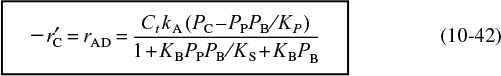
Cumene reaction rate law if adsorption were the limiting step
We now wish to sketch a plot of the initial rate of reaction as a function of the partial pressure of cumene, PC0. Initially, no products are present; consequently, PP = PB = 0. The initial rate is given by
If the cumene decomposition is adsorption rate limited, then from Equation (10-43) we see that the initial rate will be linear with the initial partial pressure of cumene, as shown in Figure 10-15.
Before checking to see if Figure 10-15 is consistent with experimental observation, we shall derive the corresponding rate laws for the other possible rate-limiting steps and then develop corresponding initial rate plots for the case when the surface reaction is rate-limiting and then for the case when the desorption of benzene is rate-limiting.
If adsorption were rate-limiting, the data should show ![]() increasing linearly with PCO.
increasing linearly with PCO.

10.3.2 Is the Surface Reaction Rate-Limiting?
The rate of surface reaction is

Single-site mechanism
Since we cannot readily measure the concentrations of the adsorbed species, we must utilize the adsorption and desorption steps to eliminate CC·S and CB·S from this equation.
From the adsorption rate expression in Equation (10-25) and the condition that kA and kD are very large by comparison with kS when the surface reaction is limiting (i.e., rAD/kA ![]() 0),12 we obtain a relationship for the surface concentration for adsorbed cumene
0),12 we obtain a relationship for the surface concentration for adsorbed cumene
12 See footnote 10 on page 424.
CC⋅S = KCPCCv
In a similar manner, the surface concentration of adsorbed benzene can be evaluated from the desorption rate expression, Equation (10-29), together with the approximation
Using ![]() to find CB·S and CC·S in terms of partial pressures
to find CB·S and CC·S in terms of partial pressures
then we get the same result for CB·S as before when we had adsorption limitation, i.e.,
CB⋅S = KBPBCv
Substituting for CB·S and CC·S in Equation (10-26) gives us

where the thermodynamic equilibrium constant was used to replace the ratio of surface reaction and adsorption constants, i.e.,
The only variable left to eliminate is Cv and we use a site balance to accomplish this, i.e.,
Site balance
Substituting for concentrations of the adsorbed species, CB·S, and CC·S, factoring out CV, and rearranging yields
Substituting for CV in Equation (10-26a)
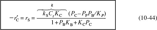
Cumene rate law for surface-reaction-limiting
The initial rate of reaction is

Figure 10-16 shows the initial rate of reaction as a function of the initial partial pressure of cumene for the case of surface-reaction-limiting.
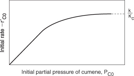
At low partial pressures of cumene
and we observe that the initial rate will increase linearly with the initial partial pressure of cumene:
At high partial pressures
and Equation (10-45) becomes
If surface reaction were rate-limiting, the data would show this behavior.
and the initial rate is independent of the initial partial pressure of cumene.
10.3.3 Is the Desorption of Benzene Rate-Limiting?
The rate expression for the desorption of benzene is
From the rate expression for surface reaction, Equation (10-26), we set
For desorption-limited reactions, both kA and kS are very large compared with kD, which is small.
to obtain
Similarly, for the adsorption step, Equation (10-25), we set
to obtain
CC·S = KCPCCv
then substitute for CC·S in Equation (10-46) to obtain
Combining Equations (10-26b), (10-29), and (10-47) gives us
where KC is the cumene adsorption constant, KS is the surface-reaction equilibrium constant, and KP is the thermodynamic gas-phase equilibrium constant, Equation (10-38), for the reaction. The expression for Cv is obtained from a site balance:
After substituting for the respective surface concentrations, we solve the site balance for Cv
Replacing Cv in Equation (10-48) by Equation (10-49) and multiplying the numerator and denominator by PP, we obtain the rate expression for desorption control
Cumene decomposition rate law if desorption were limiting
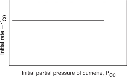
To determine the dependence of the initial rate of reaction on the initial partial pressure of cumene, we again set PP = PB = 0, and the rate law reduces to
If desorption limits, the initial rate is independent of the initial partial pressure of cumene.
with the corresponding plot of ![]() shown in Figure 10-17. If desorption were rate limiting, we would see that the initial rate of reaction would be independent of the initial partial pressure of cumene.
shown in Figure 10-17. If desorption were rate limiting, we would see that the initial rate of reaction would be independent of the initial partial pressure of cumene.
10.3.4 Summary of the Cumene Decomposition
The experimental observations of ![]() as a function of PC0 are shown in Figure 10-18. From the plot in Figure 10-18, we can clearly see that neither adsorption nor desorption is rate-limiting. For the reaction and mechanism given by
as a function of PC0 are shown in Figure 10-18. From the plot in Figure 10-18, we can clearly see that neither adsorption nor desorption is rate-limiting. For the reaction and mechanism given by
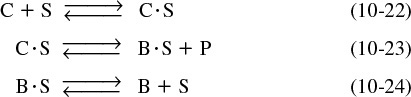
Cumene decomposition is surface-reaction-limited
Surface-reaction-limited mechanism is consistent with experimental data.
the rate law derived by assuming that the surface reaction is rate-limiting agrees with the data.
The rate law for the case of no inerts adsorbing on the surface is

The forward cumene decomposition reaction is a single-site mechanism involving only adsorbed cumene, while the reverse reaction of propylene in the gas phase reacting with adsorbed benzene is an Eley–Rideal mechanism.
If we were to have an adsorbing inert in the feed, the inert would not participate in the reaction but would occupy active sites on the catalyst surface:
Our site balance is now
Because the adsorption of the inert is at equilibrium, the concentration of sites occupied by the inert is
Substituting for the inert sites in the site balance, the rate law for surface reaction control when an adsorbing inert is present is
Adsorbing inerts
One observes that the rate decreases as the partial pressure of adsorbing inerts increases.
10.3.5 Reforming Catalysts
We now consider a dual-site mechanism, which is a reforming reaction found in petroleum refining to upgrade the octane number of gasoline.
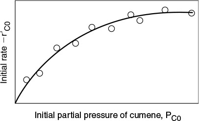
Side Note: Octane Number. Fuels with low octane numbers can produce spontaneous combustion in the car cylinder before the air/fuel mixture is compressed to its desired volume and ignited by the spark plug. The following figure shows the desired combustion wave front moving down from the spark plug and the unwanted spontaneous combustion wave in the lower right-hand corner. This spontaneous combustion produces detonation waves, which constitute engine knock. The lower the octane number, the greater the chance of spontaneous combustion and engine knock.
The octane number of a gasoline is determined from a calibration curve relating knock intensity to the % iso-octane in a mixture of iso-octane and heptane. One way to calibrate the octane number is to place a transducer on the side of the cylinder to measure the knock intensity (K.I.) (pressure pulse) for various mixtures of heptane and iso-octane. The octane number is the percentage of iso-octane in this mixture. That is, pure iso-octane has an octane number of 100, 80% iso-octane/20% heptane has an octane number of 80, and so on. The knock intensity is measured for this 80/20 mixture and recorded. The relative percentages of iso-octane and heptane are changed (e.g., 90/10), and the test is repeated. After a series of experiments, a calibration curve is constructed. The gasoline to be calibrated is then used in the test engine, where the standard knock intensity is measured. Knowing the knock intensity, the octane rating of the fuel is read off the calibration curve. A gasoline with an octane rating of 92 means that it matches the performance of a mixture of 92% iso-octane and 8% heptane. Another way to calibrate the octane number is to set the knock intensity and increase the compression ratio. A fixed percentage of iso-octane and heptane is placed in a test engine and the compression ratio (CR) is increased continually until spontaneous combustion occurs, producing an engine knock. The compression ratio and the corresponding composition of the mixture are then recorded, and the test is repeated to obtain the calibration curve of compression ratio as a function of % iso-octane. After the calibration curve is obtained, the unknown is placed in the cylinder, and the compression ratio (CR) is increased until the set knock intensity is exceeded. The CR is then matched to the calibration curve to find the octane number.
The more compact the hydrocarbon molecule, the less likely it is to cause spontaneous combustion and engine knock. Consequently, it is desired to isomerize straight-chain hydrocarbon molecules into more compact molecules through a catalytic process called reforming.
The more compact the molecule, the greater the octane number.
In the U.S., the higher the octane number the greater the cost of a gallon (liter) of gasoline. However, because of government regulations, the cost of a gallon (liter) of gasoline in Jofostan is the same for all octane numbers.
Catalyst manufacture
One common reforming catalyst is platinum on alumina. Platinum on alumina (Al2O3) (see SEM photo in Figure 10-19) is a bifunctional catalyst that can be prepared by exposing alumina pellets to a chloroplatinic acid solution, drying, and then heating in air at 775 K to 875 K for several hours. Next, the material is exposed to hydrogen at temperatures around 725 K to 775 K to produce very small clusters of Pt on alumina. These clusters have sizes on the order of 10 Å, while the alumina pore sizes on which the Pt is deposited are on the order of 100 Å to 10,000 Å (i.e., 10 nm to 1000 nm).
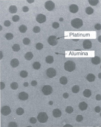
Figure 10-19 Platinum on alumina. (Masel, Richard. Chemical Kinetics and Catalysis, p. 700. © John Wiley & Sons, Inc. Reprinted by permission of John Wiley & Sons, Inc. All rights reserved.)
As an example of catalytic reforming, we shall consider the isomerization of n-pentane to i-pentane
Gasoline

Normal pentane has an octane number of 62, while iso-pentane, which is more compact, has an octane number of 90! The n-pentane adsorbs onto the platinum, where it is dehydrogenated to form n-pentene. The n-pentene desorbs from the platinum and adsorbs onto the alumina, where it is isomerized to i-pentene, which then desorbs and subsequently adsorbs onto platinum, where it is hydrogenated to form i-pentane. That is
We shall focus on the isomerization step to develop the mechanism and the rate law

The procedure for formulating a mechanism, rate-limiting step, and corresponding rate law is given in Table 10-4.
Isomerization of n-pentene (N) to i-pentene (I) over alumina
Step 1. Select a mechanism. (Let’s choose a Dual Site Mechanism)

Treat each reaction step as an elementary reaction when writing rate laws.
Reforming reaction to increase octane number of gasoline
Step 2. Assume a rate-limiting step. We choose the surface reaction first, because more than 75% of all heterogeneous reactions that are not diffusion-limited are surface-reaction-limited. We note that the PSSH must be used when more than one step is limiting (see Section 10.3.6). The rate law for the surface reaction step is
Step 3. Find the expression for concentration of the adsorbed species Ci·S. Use the other steps that are not limiting to solve for Ci·S (e.g., CN ·S and CI·S). For this reaction


Step 4. Write a site balance.
Ct = Cv + CN·S + CI·S
Step 5. Derive the rate law. Combine Steps 2, 3, and 4 to arrive at the rate law
Step 6. Compare with data. Compare the rate law derived in Step 5 with experimental data. If they agree, there is a good chance that you have found the correct mechanism and rate-limiting step. If your derived rate law (i.e., model) does not agree with the data:
a. Assume a different rate-limiting step and repeat Steps 2 through 6.
b. If, after assuming that each step is rate-limiting, none of the derived rate laws agrees with the experimental data, select a different mechanism (e.g., a single-site mechanism)

and then proceed through Steps 2 through 6.
The single-site mechanism turns out to be the correct one. For this mechanism, the rate law is
c. If two or more models agree, the statistical tests discussed in Chapter 7 (e.g., comparison of residuals) should be used to discriminate between them (see the Supplementary Reading).
We note that in Table 10-4 for the dual-site mechanism, the denominator of the rate law for –![]() is squared (i.e., in Step 5 [1/( )2)]), while for a single-site mechanism, it is not squared (i.e., Step 6 [1/( )]). This fact is useful when analyzing catalyzed reactor data.
is squared (i.e., in Step 5 [1/( )2)]), while for a single-site mechanism, it is not squared (i.e., Step 6 [1/( )]). This fact is useful when analyzing catalyzed reactor data.
TABLE 10-4 ALGORITHM FOR DETERMINING THE REACTION MECHANISM AND RATE-LIMITING STEP
Table 10-5 gives rate laws for different reaction mechanisms that are irreversible and surface-reaction-limited.

We need a word of caution at this point. Just because the mechanism and rate-limiting step may fit the rate data does not imply that the mechanism is correct.13 Usually, spectroscopic measurements are needed to confirm a mechanism absolutely. However, the development of various mechanisms and rate-limiting steps can provide insight into the best way to correlate the data and develop a rate law.
13 R. I. Masel, Principles of Adsorption and Reaction on Solid Surfaces (New York: Wiley, 1996), p. 506, www.masel.com. This is a terrific book.

10.3.6 Rate Laws Derived from the Pseudo-Steady-State Hypothesis (PSSH)
In Section 9.1 we discussed the PSSH, where the net rate of formation of reactive intermediates was assumed to be zero. An alternative way to derive a catalytic rate law rather than setting
is to assume that each species adsorbed on the surface is a reactive intermediate. Consequently, the net rate of formation of species i adsorbed on the surface will be zero
The PSSH is primarly used when more than one step is rate-limiting. The isomerization example shown in Table 10-4 is reworked using the PSSH in the Chapter 10 Expanded Material on the CRE Web site.
10.3.7 Temperature Dependence of the Rate Law
Consider a surface-reaction-limited irreversible isomerization
in which both A and B are adsorbed on the surface, and the rate law is
The specific reaction rate, k, will usually follow an Arrhenius temperature dependence and increase exponentially with temperature. However, the adsorption of all species on the surface is exothermic. Consequently, the higher the temperature, the smaller the adsorption equilibrium constant. That is, as the temperature increases, KA and KB decrease resulting in less coverage of the surface by A and B. Therefore, at high temperatures, the denominator of catalytic rate laws approaches 1. That is, at high temperatures (low coverage)
The rate law could then be approximated as
Neglecting the adsorbed species at high temperatures
or for a reversible isomerization we would have

Algorithm
Deduce
Rate law
Find
Mechanism
Evaluate
Rate-law parameters
Design
PBR
CSTR
The algorithm we can use as a start in postulating a reaction mechanism and rate-limiting step is shown in Table 10-4. Again, we can never really prove a mechanism to be correct by comparing the derived rate law with experimental data. Independent spectroscopic experiments are usually needed to confirm the mechanism. We can, however, prove that a proposed mechanism is inconsistent with the experimental data by following the algorithm in Table 10-4. Rather than taking all the experimental data and then trying to build a model from the data, Box et al. describe techniques of sequential data collection and model building.14
14 G. E. P. Box, W. G. Hunter, and J. S. Hunter, Statistics for Engineers (New York: Wiley, 1978).
10.4 Heterogeneous Data Analysis for Reactor Design
In this section we focus on four operations that chemical reaction engineers need to be able to accomplish:
(1) Developing an algebraic rate law consistent with experimental observations,
(2) Analyzing the rate law in such a manner that the rate-law parameters (e.g., k, KA) can readily be determined from the experimental data,
(3) Finding a mechanism and rate-limiting step consistent with the experimental data
(4) Designing a catalytic reactor to achieve a specified conversion
We shall use the hydrodemethylation of toluene to illustrate these four operations.
Hydrogen and toluene are reacted over a solid mineral catalyst containing clinoptilolite (a crystalline silica-alumina) to form methane and benzene15
15 J. Papp, D. Kallo, and G. Schay, J. Catal., 23, 168.
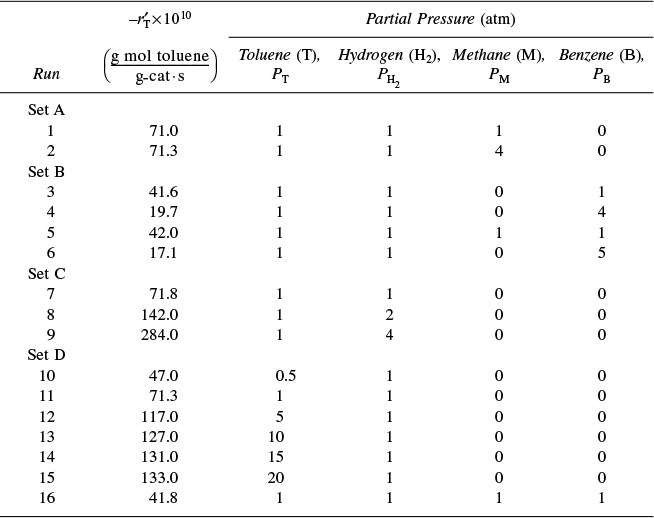
We wish to design a packed-bed reactor and a fluidized CSTR to process a feed consisting of 30% toluene, 45% hydrogen, and 25% inerts. Toluene is fed at a rate of 50 mol/min at a temperature of 640°C and a pressure of 40 atm (4052 kPa). To design the PBR, we must first determine the rate law from the differential reactor data presented in Table 10-6. In this table, we are given the rate of reaction of toluene as a function of the partial pressures of hydrogen (H2), toluene (T), benzene (B), and methane (M). In the first two runs, methane was introduced into the feed together with hydrogen and toluene, while the other product, benzene, was fed to the reactor together with the reactants only in runs 3, 4, and 6. In runs 5 and 16, both methane and benzene were introduced in the feed. In the remaining runs, none of the products was present in the feedstream. Because the conversion was less than 1% in the differential reactor, the partial pressures of the products, methane and benzene, formed in these runs were essentially zero, and the reaction rates were equivalent to initial rates of reaction.
Unscramble the data to find the rate law
10.4.1 Deducing a Rate Law from the Experimental Data
First, let’s look at run 3. In run 3, there is no possibility of the reverse reaction taking place because the concentration of methane is zero, i.e., PM = 0, whereas in run 5 the reverse reaction could take place because all products are present. Comparing runs 3 and 5, we see that the initial rate is essentially the same for both runs, and we can assume that the reaction is essentially irreversible.
We now ask what qualitative conclusions can be drawn from the data about the dependence of the rate of disappearance of toluene, ![]() , on the partial pressures of toluene, hydrogen, methane, and benzene.
, on the partial pressures of toluene, hydrogen, methane, and benzene.
1. Dependence on the product methane. If methane were adsorbed on the surface, the partial pressure of methane would appear in the denominator of the rate expression and the rate would vary inversely with methane concentration

However, comparing runs 1 and 2 we observe that a fourfold increase in the pressure of methane has little effect on ![]() . Consequently, we assume that methane is either very weakly adsorbed (i.e., KMPM
. Consequently, we assume that methane is either very weakly adsorbed (i.e., KMPM ![]() 1) or goes directly into the gas phase in a manner similar to propylene in the cumene decomposition previously discussed.
1) or goes directly into the gas phase in a manner similar to propylene in the cumene decomposition previously discussed.
If it is in the denominator, it is probably on the surface.
2. Dependence on the product benzene. In runs 3 and 4, we observe that, for fixed concentrations (partial pressures) of hydrogen and toluene, the rate decreases with increasing concentration of benzene. A rate expression in which the benzene partial pressure appears in the denominator could explain this dependency
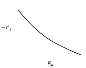
The type of dependence of ![]() on PB given by Equation (10-68) suggests that benzene is adsorbed on the clinoptilolite surface.
on PB given by Equation (10-68) suggests that benzene is adsorbed on the clinoptilolite surface.
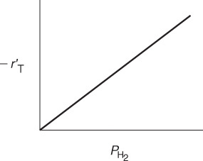
3. Dependence on toluene. At low concentrations of toluene (runs 10 and 11), the rate increases with increasing partial pressure of toluene, while at high toluene concentrations (runs 14 and 15), the rate is virtually independent of the toluene partial pressure. A form of the rate expression that would describe this behavior is

A combination of Equations (10-68) and (10-69) suggests that the rate law may be of the form
4. Dependence on hydrogen. When we compare runs 7, 8, and 9 in Table 10-6, we see that the rate increases linearly with increasing hydrogen concentration, and we conclude that the reaction is first order in H2. In light of this fact, hydrogen is either not adsorbed on the surface or its coverage of the surface is extremely low (1 » KH2PH2) for the pressures used. If H2 were adsorbed, ![]() would have a dependence on PH2 analogous to the dependence of
would have a dependence on PH2 analogous to the dependence of ![]() on the partial pressure of toluene, PT [see Equation (10-69)]. For first-order dependence on H2,
on the partial pressure of toluene, PT [see Equation (10-69)]. For first-order dependence on H2,
Combining Equations (10-67) through (10-71), we find that the rate law
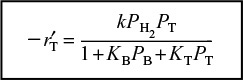
is in qualitative agreement with the data shown in Table 10-6.
10.4.2 Finding a Mechanism Consistent with Experimental Observations
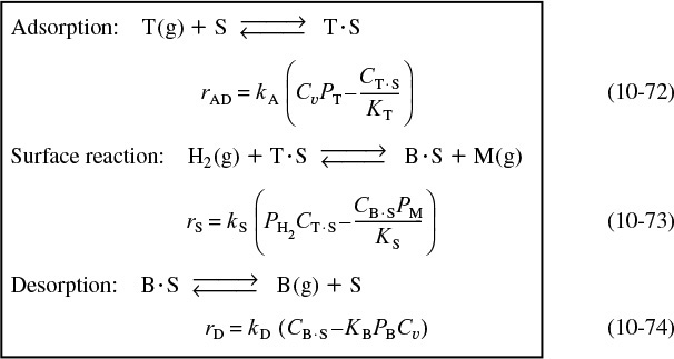
We now propose a mechanism for the hydrodemethylation of toluene. We assume that the reaction follows an Eley-Rideal mechanism where toluene is adsorbed on the surface and then reacts with hydrogen in the gas phase to produce benzene adsorbed on the surface and methane in the gas phase. Benzene is then desorbed from the surface. Because approximately 75% to 80% of all heterogeneous reaction mechanisms are surface-reaction-limited rather than adsorption- or desorption-limited, we begin by assuming the reaction between adsorbed toluene and gaseous hydrogen to be reaction-rate-limited. Symbolically, this mechanism and associated rate laws for each elementary step are
Approximately 75% of all heterogeneous reaction mechanisms are surface-reaction-limited.
Proposed Mechanism
Eley–Rideal mechanism
For surface-reaction-limited mechanisms
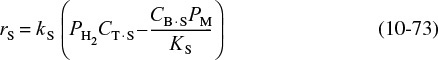
we see that we need to replace CT·S and CB·S in Equation (10-73) by quantities that we can measure.
For surface-reaction-limited mechanisms, we use the adsorption rate Equation (10-72) for toluene to obtain CT·S16, i.e.,
16 See footnote 10 on page 424.
Then
and we use the desorption rate Equation (10-74) for benzene to obtain CB·S:
Then
The total concentration of sites is
Perform a site balance to obtain Cv.
Substituting Equations (10-75) and (10-76) into Equation (10-77) and rearranging, we obtain
Next, substitute for CT·S and CB·S, and then substitute for Cv in Equation (10-73) to obtain the rate law for the case when the reaction is surface-reaction-rate-limited
We have shown by comparing runs 3 and 5 that we can neglect the reverse reaction, i.e., the thermodynamic equilibrium constant KP is very, very large. Consequently, we obtain

Rate law for Eley–Rideal surface-reaction-limited mechanism
Again we note that the adsorption equilibrium constant of a given species is exactly the reciprocal of the desorption equilibrium constant of that species.
10.4.3 Evaluation of the Rate-Law Parameters
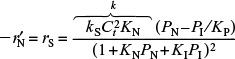
In the original work on this reaction by Papp et al.,17 over 25 models were tested against experimental data, and it was concluded that the preceding mechanism and rate-limiting step (i.e., the surface reaction between adsorbed toluene and H2 gas) is the correct one. Assuming that the reaction is essentially irreversible, the rate law for the reaction on clinoptilolite is
17 Ibid.

We now wish to determine how best to analyze the data to evaluate the rate-law parameters, k, KT, and KB. This analysis is referred to as parameter estimation.18 We now rearrange our rate law to obtain a linear relationship between our measured variables. For the rate law given by Equation (10-80), we see that if both sides of Equation (10-80) are divided by PH2PT and the equation is then inverted
18 See the Supplementary Reading (page 492) for a variety of techniques for estimating the rate-law parameters.
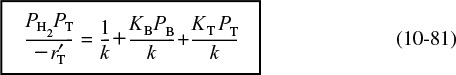
Linearize the rate equation to extract the rate-law parameters.
The regression techniques described in Chapter 7 could be used to determine the rate-law parameters by using the equation
A linear least-squares analysis of the data shown in Table 10-6 is presented on the CRE Web site.
One can use the linearized least-squares analysis (PRS 7.3) to obtain initial estimates of the parameters k, KT, KB, in order to obtain convergence in nonlinear regression. However, in many cases it is possible to use a nonlinear regression analysis directly, as described in Sections 7.5 and 7.6, and in Example 10-1.
Example 10–1 Nonlinear Regression Analysis to Determine the Model Parameters k, KB, and KT
(a) Use nonlinear regression, as discussed in Chapter 7, along with the data in Table 10-6, to find the best estimates of the rate-law parameters k, KB, and KT in Equation (10-80).
(b) Write the rate law solely as a function of the partial pressures.
(c) Find the ratio of the sites occupied by toluene, CT•S, to those occupied by benzene, CB•S, at 40% conversion of toluene.
Solution
The data from Table 10-6 were entered into the Polymath nonlinear least-squares program with the following modification. The rates of reaction in column 1 were multiplied by 1010, so that each of the numbers in column 1 was entered directly (i.e., 71.0, 71.3, ...). The model equation was

Following the step-by-step regression procedure in Chapter 7 and on the CRE Web site Summary Notes, we arrive at the following parameter values shown in Table E10-1.1.

(a) The best estimates are shown in the upper-right-hand box of Table E10-1.1.
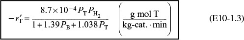
(b) Converting the rate law to kilograms of catalyst and minutes,
we have
Ratio of sites occupied by toluene to those occupied by benzene
(c) After we have the adsorption constants, KT and KB, we can calculate the ratio of sites occupied by the various adsorbed species. For example, taking the ratio of Equation (10-75) to Equation (10-76), the ratio of toluene-occupied sites to benzeneoccupied sites at 40% conversion is
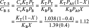
We see that at 40% conversion there are approximately 12% more sites occupied by toluene than by benzene. This fact is common knowledge to every chemical engineering student at Jofostan University, Riça, Jofostan.
Analysis: This example shows once again how to determine the values of rate-law parameters from experimental data using Polymath regression. It also shows how to calculate the different fraction of sites, both vacant and occupied, as a function of conversion.
10.4.4 Reactor Design
Our next step is to express the partial pressures PT, PB, and PH2 as a function of X, combine the partial pressures with the rate law, ![]() , as a function of conversion, and carry out the integration of the packed-bed design equation
, as a function of conversion, and carry out the integration of the packed-bed design equation
Example 10–2 Catalytic Reactor Design
The hydrodemethylation of toluene is to be carried out in a PBR catalytic reactor.
The molar feed rate of toluene to the reactor is 50 mol/min, and the reactor inlet is at 40 atm and 640°C. The feed consists of 30% toluene, 45% hydrogen, and 25% inerts. Hydrogen is used in excess to help prevent coking. The pressure-drop parameter, α, is 9.8 × 10⁻⁵ kg–1.
(a) Plot and analyze the conversion, the pressure ratio, p, and the partial pressures of toluene, hydrogen, and benzene as a function of PBR catalyst weight.
(b) Determine the catalyst weight in a fluidized CSTR with a bulk density of 400 kg/m3 (0.4 g/cm3) to achieve 65% conversion.
Solution
(a) PBR with pressure drop
1. Mole Balance:

Balance on toluene (T)
2. Rate Law: From Equation (E10-1.1) we have
with k = 0.00087 mol/atm2/kg-cat/min, KB = 1.39 atm–1, and KT = 1.038 atm–1.
3. Stoichiometry:

Relating Toluene (T) Benzene (B) Hydrogen (H2)
Because ε = 0, we can use the integrated form of the pressure-drop term.

P0 = total pressure at the entrance
Note that PT0 designates the inlet partial pressure of toluene. In this example, the inlet total pressure is designated P0 to avoid any confusion. The inlet mole fraction of toluene is 0.3 (i.e., yT0 = 0.3), so that the inlet partial pressure of toluene is
PT0 = (0.3)(40) = 12 atm
Pressure drop in PBRs is discussed in Section 5.5.
We now calculate the maximum catalyst weight we can have, such that the exiting pressure will not fall below atmospheric pressure (i.e., 1.0 atm) for the specified feed rate. This weight is calculated by substituting the entering pressure of 40 atm and the exiting pressure of 1 atm into Equation (5-33), i.e.,

4. Evaluate: Consequently, we will set our final weight at 10,000 kg and determine the conversion profile as a function of catalyst weight up to this value. Equations (E10-2.1) through (E10-2.5) are shown in the Polymath program in Table E10-2.1. The conversion is shown as a function of catalyst weight in Figure E10-2.1, and profiles of the partial pressures of toluene, hydrogen, and benzene are shown in Figure E10-2.2. We note that the pressure drop causes (cf. Equation E10-2.5) the partial pressure of benzene to go through a maximum as one traverses the reactor.
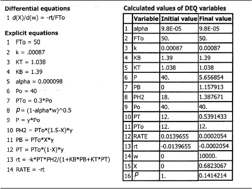
Conversion profile down the packed bed
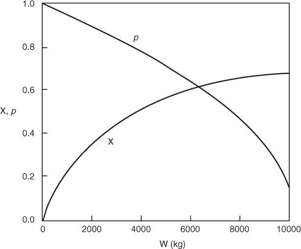

Note the partial pressure of benzene goes through a maximum. Why?
PBR Analysis: For the case of no pressure drop, the conversion that would have been achieved with 10,000 kg of catalyst would have been 79%, compared with 68.2% when there is pressure drop in the reactor. To carry out this calculation, use the Living Example Program (LEP) on the CRE Web site and simply multiply the pressure-drop parameter by zero, i.e., line (5) would read α = 0.00098*0. For the feed rate given, eliminating or minimizing pressure drop would increase the production of benzene by up to 61 million pounds per year! Finally, we note in Figure E10-2.2 that the partial pressure of benzene (PB) goes through a maximum. This maximum can be explained by recalling that PB is just the product of the benzene mole fraction (yB) times the total pressure (P) [i.e., PB = yBPT]. Near the middle to end of the bed, benzene is no longer being formed so that yB stops increasing. However, because of the pressure drop, the total pressure decreases and, as a result, so does PB.
If one had neglected ΔP it could have been very embarrassing.
See YouTube video, “Reaction Engineering Gone Wrong,” accessible from the CRE Web site home page.
(b) Fluidized CSTR
We will now calculate the fluidized CSTR catalyst weight necessary to achieve the same (ca.) conversion as in the packed-bed reactor at the same operating conditions. The bulk density in the fluidized reactor is 0.4 g/cm3. The design equation is
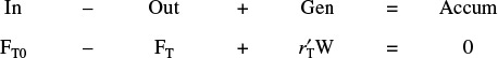
Rearranging
Fluidized CSTR
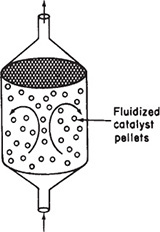
2. Rate Law and 3. Stoichiometry same as in part (a) PBR calculation
4. Combine and Evaluate: Writing Equation (E10-2.2) in terms of conversion (E10-2.3) and then substituting X = 0.65 and PT0 = 12 atm, we have
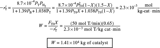
The corresponding reactor volume is
Analysis: This example used real data and the CRE algorithm to design a PBR and CSTR. An important point is that it showed how one could be embarrassed by not including pressure drop in the design of a packed-bed reactor. We also note that for both the PBR and fluidized CSTR, the values of the catalyst weight and reactor volume are quite high, especially for the low feed rates given. Consequently, the temperature of the reacting mixture should be increased to reduce the catalyst weight, provided that side reactions and catalyst decay do not become a problem at higher temperatures.
How can the weight of catalyst be reduced? Raise the temperature?
Example 10-2 illustrated the major activities pertinent to catalytic reactor design described earlier in Figure 10-6. In this example, the rate law was extracted directly from the data and then a mechanism was found that was consistent with experimental observation. Conversely, developing a feasible mechanism may guide one in the synthesis of the rate law.
10.5 Reaction Engineering in Microelectronic Fabrication
10.5.1 Overview
We now extend the principles of the preceding sections to one of the emerging technologies in chemical engineering. Chemical engineers are now playing an important role in the electronics industry. Specifically, they are becoming more involved in the manufacture of electronic and photonic devices, recording materials, and especially medical lab-on-a-chip devices.

Surface reactions play an important role in the manufacture of microelectronic devices. One of the single most important developments of the twentieth century was the invention of the integrated circuit. Advances in the development of integrated circuitry have led to the production of circuits that can be placed on a single semiconductor chip the size of a pinhead and perform a wide variety of tasks by controlling the electron flow through a vast network of channels. These channels, which are made from semiconductors such as silicon, gallium arsenide, indium phosphide, and germanium, have led to the development of a multitude of novel microelectronic devices. Examples of microelectronic sensing devices manufactured using chemical reaction engineering principles are shown in the left-hand margin.
The manufacture of an integrated circuit requires the fabrication of a network of pathways for electrons. The principal reaction engineering steps of the fabrication process include depositing material on the surface of a material called a substrate (e.g., by chemical vapor deposition, abbreviated as CVD), changing the conductivity of regions of the surface (e.g., by boron doping or ion inplantation), and removing unwanted material (e.g., by etching). By applying these steps systematically, miniature electronic circuits can be fabricated on very small semiconductor chips. The fabrication of microelectronic devices may include as few as 30 or as many as 200 individual steps to produce chips with up to 109 elements per chip.

An abbreviated schematic of the steps involved in producing a typical metal-oxide, semiconductor, field-effect transistor (MOSFET) device is shown in Figure 10-20. Starting from the upper left, we see that single-crystal silicon ingots are grown in a Czochralski crystallizer, sliced into wafers, and chemically and physically polished. These polished wafers serve as starting materials for a variety of microelectronic devices. A typical fabrication sequence is shown for processing the wafer, beginning with the formation of an SiO2 layer on top of the silicon. The SiO2 layer may be formed either by oxidizing a silicon layer or by laying down a SiO2 layer by chemical vapor deposition (CVD). Next, the wafer is masked with a polymer photoresist, a template with the pattern to be etched onto the SiO2 layer is placed over the photoresist, and the wafer is exposed to ultraviolet irradiation. If the mask is a positive photoresist, the light will cause the exposed areas of the polymer to dissolve when the wafer is placed in the developer. On the other hand, when a negative photoresist mask is exposed to ultraviolet irradiation, cross-linking of the polymer chains occurs, and the unexposed areas dissolve in the developer. The undeveloped portion of the photoresist (in either case) will protect the covered areas from etching.
Chemical engineering principles are involved in virtually every step!
After the exposed areas of SiO2 are etched to form trenches (either by wet etching or by plasma etching), the remaining photoresist is removed. Next, the wafer is placed in a furnace containing gas molecules of the desired dopant, which then diffuse into the exposed silicon. After diffusion of dopant to the desired depth in the wafer, the wafer is removed and then SiO2 is removed by etching. The sequence of masking, etching, CVD, and metallization continues until the desired device is formed. A schematic of a final chip is shown in the lower-right-hand corner of Figure 10-20. In Section 10.5.2, we discuss one of the key processing steps, CVD.
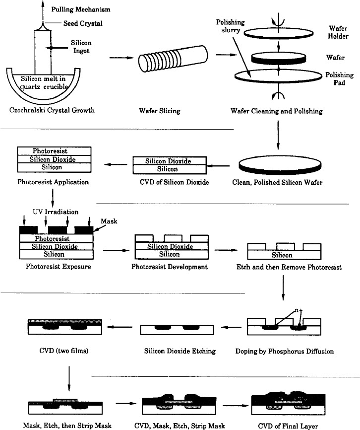
10.5.2 Chemical Vapor Deposition
The mechanisms by which CVD occurs are very similar to those of heterogeneous catalysis discussed earlier in this chapter. The reactant(s) adsorbs on the surface and then reacts on the surface to form a new surface. This process may be followed by a desorption step, depending on the particular reaction.
Ge used in solar cells
The growth of a germanium epitaxial film as an interlayer between a gallium arsenide layer and a silicon layer has received attention in the microelectronics industry.19 Epitaxial germanium is also an important material in the fabrication of tandem solar cells. The growth of germanium films can be accomplished by CVD. A proposed mechanism is
19 H. Ishii and Y. Takahashi, J. Electrochem. Soc., 135, p. 1539.
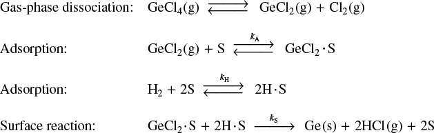
Mechanism
At first it may appear that a site has been lost when comparing the right- and left-hand sides of the surface reaction step. However, the newly formed germanium atom on the right-hand side is a site for the future adsorption of H2 (g) or GeCl2 (g), and there are three sites on both the right- and left-hand sides of the surface reaction step. These sites are shown schematically in Figure 10-21.

The surface reaction between adsorbed molecular hydrogen and germanium dichloride is believed to be rate-limiting. The reaction follows an elementary rate law with the rate being proportional to the fraction of the surface covered by GeCl2 times the square of the fraction of the surface covered by molecular hydrogen.

Rate law for rate-limiting step
The deposition rate (film growth rate) is usually expressed in nanometers per second and is easily converted to a molar rate (mol/m2 · s) by multiplying by the molar density of solid germanium (mol/m3).
The difference between developing CVD rate laws and rate laws for catalysis is that the site concentration (e.g., Cv) is replaced by the fractional surface area coverage (e.g., the fraction of the surface that is vacant, fv). The total fraction of surface available for adsorption should, of course, add up to 1.0.
Area balance
We will first focus our attention on the adsorption of GeCl2. The rate of jumping on to the surface is proportional to the partial pressure of GeCl2, PGeCl2, and the fraction of the surface that is vacant, fv. The net rate of GeCl2 adsorption is
Since the surface reaction is rate-limiting, in a manner analogous to catalysis reactions, we have for the adsorption of GeCl2
Adsorption of GeCl2 not rate-limiting
Solving Equation (10-84) for the fractional surface coverage of GeCl2 gives

For the dissociative adsorption of hydrogen on the Ge surface, the equation analogous to Equation (10-84) is
Since the surface reaction is rate-limiting
Adsorption of H2 is not rate-limiting
Then
Recalling the rate of deposition of germanium, we substitute for fGeCl2 and fH in Equation (10-82) to obtain
We solve for fv in an identical manner to that for Cv in heterogeneous catalysis. Substituting Equations (10-85) and (10-87) into Equation (10-83) gives
Rearranging yields

Finally, substituting for fv in Equation (10-88), we find that

and lumping KA, KH, and kS into a specific reaction rate k’ yields
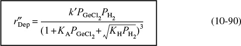
Rate of deposition of Ge
We now need to relate the partial pressure of GeCl2 to the partial pressure of GeCl4 in order to calculate the conversion of GeCl4. If we assume that the gas-phase reaction
Equilibrium in gas phase
is in equilibrium, we have

and if hydrogen is weakly adsorbed (![]() ), we obtain the rate of deposition as
), we obtain the rate of deposition as
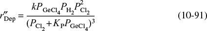
Rate of deposition of Ge when H2 is weakly adsorbed
We now can use stoichiometry to express each of the species’ partial pressures in terms of conversion and the entering partial pressure of GeCl4, PGeCl4,0, and then proceed to calculate the conversion.
It should also be noted that it is possible that GeCl2 may also be formed by the reaction of GeCl4 and a Ge atom on the surface, in which case a different rate law would result.
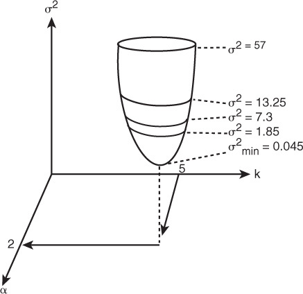
Regression
10.6 Model Discrimination
We have seen that for each mechanism and each rate-limiting step we can derive a rate law. Consequently, if we had three possible mechanisms and three rate-limiting steps for each mechanism, we would have nine possible rate laws to compare with the experimental data. We will use the regression techniques discussed in Chapter 7 to identify which model equation best fits the data by choosing the one with the smaller sums of squares and/or carrying out an F-test. We could also compare the residual plots for each model, which not only show the error associated with each data point but also show if the error is randomly distributed or if there is a trend in the error. If the error is randomly distributed, this result is an additional indication that the correct rate law has been chosen.
We need to raise a caution here about choosing the model with the smallest sums of squares. The caution is that the model parameter values that give the smallest sum must be realistic. In the case of heterogeneous catalysis, all values of the adsorption equilibrium constants must be positive. In addition, if the temperature dependence is given, because adsorption is exothermic, the adsorption equilibrium constant must decrease with increasing temperature. To illustrate these principles, let’s look at the following example.
Example 10–3 Hydrogenation of Ethylene to Ethane
The hydrogenation (H) of ethylene (E) of form ethane (EA),
H2 + C2H4 → C2H6
is carried out over a cobalt molybdenum catalyst [Collect. Czech. Chem. Commun., 51, 2760 (1988)]. Carry out a nonlinear regression analysis on the data given in Table E10-3.1, and determine which rate law best describes the data.

Procedure
• Enter data
• Enter model
• Make initial estimates of parameters
• Run regression
• Examine parameters and variance
• Observe error distribution
• Choose model
Determine which of the following rate laws best describes the data in Table E10-3.1.
(a) ![]()
(b) ![]()
(c) ![]()
(d) ![]()

Solution
Polymath was chosen as the software package to solve this problem. The data in Table E10-3.1 were entered into the program. A screen-shot-by-screen-shot set of instructions on how to carry out the regression is given on the CRE Web site, at the end of the Summary Notes for Chapter 7. After entering the data and following the step-by-step procedures, the results shown in Table E10-3.2 were obtained.

Model (a) Single site, surface-reaction, rate-limited with hydrogen weakly adsorbed
From Table E10-3.2 data, we can obtain
We now examine the sums of squares (variance) and range of variables themselves. The sums of squares is reasonable and, in fact, the smallest of all the models at 0.0049. However, let’s look at KEA. We note that the value for the 95% confidence limit of ±0.0636 is greater than the nominal value of KEA = 0.043 atm–1 itself (i.e., KEA = 0.043 ± 0.0636). The 95% confidence limit means that if the experiment were run 100 times and then 95 times it would fall within the range (–0.021) < KEA < (0.1066). Because KEA can never be negative, we are going to reject this model. Consequently, we set KEA = 0 and proceed to Model (b).
Model (b) Single site, surface-reaction, rate-limited with ethane and hydrogen weakly adsorbed
From Table E10-3.2 we can obtain
The value of the adsorption constant KE = 2.1 atm–1 is reasonable and is not negative within the 95% confidence limit. Also, the variance is small at ![]() .
.
Model (c) Dual site, surface-reaction, rate-limited with hydrogen and ethane weakly adsorbed
From Table E10-3.2 we can obtain

While KE is small, it never goes negative within the 95% confidence interval. The variance of this model at ![]() is much larger than the other models. Comparing the variance of model (c) with model (b)
is much larger than the other models. Comparing the variance of model (c) with model (b)
We see that the ![]() is an order of magnitude greater than
is an order of magnitude greater than ![]() , and therefore we eliminate model (c).20
, and therefore we eliminate model (c).20
20 See G. F. Froment and K. B. Bishoff, Chemical Reaction Analysis and Design, 2nd ed. (New York: Wiley, 1990), p. 96.
Model (d) Empirical
Similarly for the power law model, we obtain from Table E10-3.2
As with model (c), the variance is quite large compared to model (b)
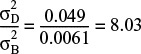
So we also eliminate model (d). For heterogeneous reactions, Langmuir-Hinshelwood rate laws are preferred over power-law models.
Analysis: Choose the Best Model. In this example, we were presented with four rate laws and were asked which law best fits the data. Because all the parameter values are realistic for model (b) and the sums of squares are significantly smaller for model (b) than for the other models, we choose model (b). We note again that there is a caution we need to point out regarding the use of regression! One cannot simply carry out a regression and then choose the model with the lowest value of the sums of squares. If this were the case, we would have chosen model (a), which had the smallest sums of squares of all the models with σ2 = 0.0049. However, one must consider the physical realism of the parameters in the model. In model (a) the 95% confidence interval was greater than the parameter itself, thereby yielding negative values of the parameter, KAE, which is physically impossible.
10.7 Catalyst Deactivation
In designing fixed and ideal fluidized-bed catalytic reactors, we have assumed up to now that the activity of the catalyst remains constant throughout the catalyst’s life. That is, the total concentration of active sites, Ct, accessible to the reaction does not change with time. Unfortunately, Mother Nature is not so kind as to allow this behavior to be the case in most industrially significant catalytic reactions. One of the most insidious problems in catalysis is the loss of catalytic activity that occurs as the reaction takes place on the catalyst. A wide variety of mechanisms have been proposed by Butt and Petersen, to explain and model catalyst deactivation.21
21 J. B. Butt and E. E. Petersen, Activation, Deactivation and Poisoning of Catalysts (New York: Academic Press, 1988).
Catalytic deactivation adds another level of complexity to sorting out the reaction rate law parameters and pathways. In addition, we need to make adjustments for the decay of the catalysts in the design of catalytic reactors. However, please don’t worry, this adjustment is usually made by a quantitative specification of the catalyst’s activity, a (t). In analyzing reactions over decaying catalysts, we divide the reactions into two categories: separable kinetics and nonseparable kinetics. In separable kinetics, we separate the rate law and activity
Separable kinetics: –![]() = a (Past history) × –
= a (Past history) × –![]() (Fresh catalyst)
(Fresh catalyst)
When the kinetics and activity are separable, it is possible to study catalyst decay and reaction kinetics independently. However, nonseparability
Nonseparable kinetics: –![]() = –
= –![]() (Past history, fresh catalyst)
(Past history, fresh catalyst)
must be accounted for by assuming the existence of a nonideal surface or by describing deactivation by a mechanism composed of several elementary steps.22
22 D. T. Lynch and G. Emig, Chem. Eng. Sci., 44(6), 1275–1280 (1989).
We shall consider only separable kinetics and define the activity of the catalyst at time t, a (t), as the ratio of the rate of reaction on a catalyst that has been used for a time t to the rate of reaction on a fresh catalyst (t = 0):
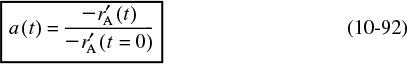
a (t): catalyst activity
Because of the catalyst decay, the activity decreases with time and a typical curve of the activity as a function of time is shown in Figure 10-22.
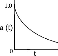
Combining Equations (10-92) and (3-2), the rate of disappearance of reactant A on a catalyst that has been utilized for a time t is

Reaction rate law accounting for catalyst activity

The rate of catalyst decay, rd, can be expressed in a rate law analogous to Equation (10-93)
Catalyst decay rate law
where p[a(t)] is some function of the catalyst activity, kd is the specific decay constant, and h (Ci) is the functionality of rate of decay, rd, on the reacting species concentrations. For the cases presented in this chapter, this functionality either will be independent of concentration (i.e., h = 1) or will be a linear function of species concentration (i.e., h = Ci).
e.g., p[a(t)] = [a(t)]2
The functionality of the activity term, p[a(t)], in the decay law can take a variety of forms. For example, for a first-order decay
and for a second-order decay
The particular function, p (a), will vary with the gas catalytic system being used and the reason or mechanism for catalytic decay.
10.7.1 Types of Catalyst Deactivation
There are three categories into which the loss of catalytic activity can traditionally be divided: sintering or aging, fouling or coking, and poisoning.
• Sintering
• Fouling
• Poisoning
Deactivation by Sintering (Aging).23 Sintering, also referred to as aging, is the loss of catalytic activity due to a loss of active surface area resulting from the prolonged exposure to high gas-phase temperatures. The active surface area may be lost either by crystal agglomeration and growth of the metals deposited on the support or by narrowing or closing of the pores inside the catalyst pellet. A change in the surface structure may also result from either surface recrystallization or the formation or elimination of surface defects (active sites). The reforming of heptane over platinum on alumina is an example of catalyst deactivation as a result of sintering.
23 See G. C. Kuczynski, ed., Sintering and Catalysis, vol. 10 of Materials Science Research (New York: Plenum Press, 1975).
Figure 10-23 shows the loss of surface area resulting from the flow of the solid porous catalyst support at high temperatures to cause pore closure. Figure 10-24 shows the loss of surface area by atomic migration and agglomeration of small metal sites deposited on the surface into a larger site where the interior atoms are not accessible to the reaction. Sintering is usually negligible at temperatures below 40% of the melting temperature of the solid.24
24 R. Hughes, Deactivation of Catalysts (San Diego: Academic Press, 1984).
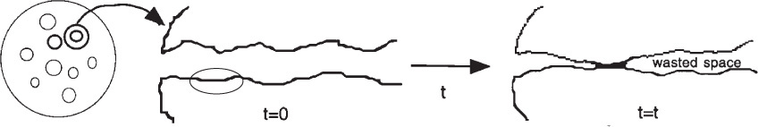
The catalyst support becomes soft and flows, resulting in pore closure.
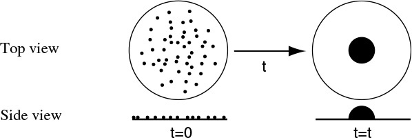
Figure 10-24 Decay by sintering: agglomeration of deposited metal sites; loss of reactive surface area.
The atoms move along the surface and agglomerate.
Deactivation by sintering may in some cases be a function of the mainstream gas concentration. Although other forms of the sintering decay rate laws exist, one of the most commonly used decay laws is second order with respect to the present activity
Integrating, with a = 1 at time t = 0, yields
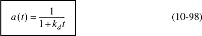
Sintering: second-order decay
The amount of sintering is usually measured in terms of the active surface area of the catalyst Sa
The sintering decay constant, kd, follows the Arrhenius equation
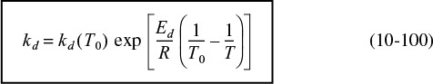
The decay activation energy, Ed, for the reforming of heptane on Pt/Al2O3 is on the order of 70 kcal/mol, which is rather high. As mentioned earlier, sintering can be reduced by keeping the temperature below 0.3 to 0.4 times the metal’s melting point.
Minimizing sintering
We will now stop and consider reactor design for a fluid–solid system with decaying catalyst. To analyze these reactors, we only add one step to our algorithm; that is, determine the catalyst decay law. The sequence is shown here.

The algorithm
Example 10–4 Calculating Conversion with Catalyst Decay in Batch Reactors
The first-order isomerization
is being carried out isothermally in a batch reactor on a catalyst that is decaying as a result of aging. Derive an equation for conversion as a function of time.
Solution
1. Mol Balance:
where Xd is the conversion of A when the catalyst is decaying.
2. Reaction-Rate Law:
3. Decay Law: For second-order decay by sintering:
One extra step (number 3) is added to the algorithm.
4. Stoichiometry:
5. Combining gives us
Let k = k’W/V. Substituting for catalyst activity a, we have
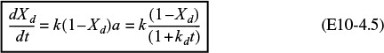
where Xd is the conversion when there is decay. We want to compare the conversion with and without catalyst decay.
For no decay kd = 0
The Polymath program and a comparison of the conversion with decay Xd and without decay X are shown below.
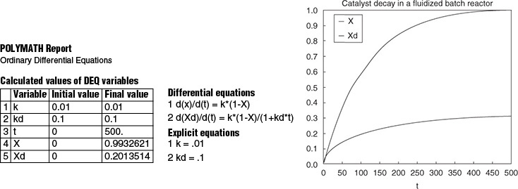
One can also obtain an analytical solution for this reaction order and low decay. Separating variables and integrating yields

6. Solving for the conversion Xd at any time t, we find that
the analytical solution without decay
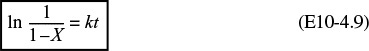
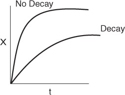
Analysis: One observes that for long times the conversion with decay approaches a rather flat plateau and reaches conversion of about 30%. This is the conversion that will be achieved in a batch reactor for a first-order reaction when the catalyst decay law is second order. By comparison, we obtain virtually complete conversion in 500 minutes when there is no decay. The purpose of this example was to demonstrate the algorithm for isothermal catalytic reactor design for a decaying catalyst. In problem P10-1B(d) you are asked to sketch the temperature–time trajectories for various values of k and kd.
Deactivation by Coking or Fouling. This mechanism of decay (see Figures 10-25 and 10-26) is common to reactions involving hydrocarbons. It results from a carbonaceous (coke) material being deposited on the surface of a catalyst.
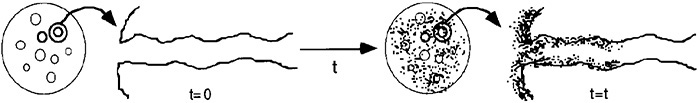
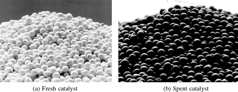
Figure 10-26 Decay by coking. (Photos courtesy of Engelhard catalyst, copyright by Michael Gaffney Photographer, Mendham, NJ.)
The amount of coke on the surface after a time t has been found to obey the following empirical relationship
where CC is the concentration of carbon on the surface (g/m2) and n and A are fouling parameters, which can be functions of the feed rate. This expression was originally developed by Voorhies and has been found to hold for a wide variety of catalysts and feed streams.25 Representative values of A and n for the cracking of East Texas light gas oil yield26
25 A. Voorhies, Ind. Eng. Chem., 37, 318 (1945).
26 C. O. Prater and R. M. Lago, Adv. Catal., 8, 293 (1956).
Different functionalities between the activity and amount of coke on the surface have been observed. One commonly used form is
or, in terms of time, we combine Equations (10-101) and (10-102)
For light Texas gas oil being cracked at 750°F over a synthetic catalyst for short times, the decay law is

where t is in seconds.
Activity for deactivation by coking
Other commonly used forms are
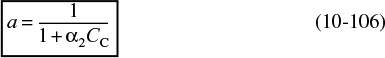
A dimensionless fouling correlation has been developed by Pacheco and Petersen.27
27 M. A. Pacheco and E. E. Petersen, J. Catal., 86, 75 (1984).
When possible, coking can be reduced by running at elevated pressures (2000 to 3000 kPa) and hydrogen-rich streams. A number of other techniques for minimizing fouling are discussed by Bartholomew.28 Catalysts deactivated by coking can usually be regenerated by burning off the carbon.
28 R. J. Farrauto and C. H. Bartholomew, Fundamentals of Industrial Catalytic Processes, 2nd edition (New York: Blackie Academic and Professional, 2006). This book is one of the most definitive resources on catalyst decay.
Minimizing coking
Deactivation by Poisoning. Deactivation by this mechanism occurs when the poisoning molecules become irreversibly chemisorbed to active sites, thereby reducing the number of sites available for the main reaction. The poisoning molecule, P, may be a reactant and/or a product in the main reaction, or it may be an impurity in the feed stream.
It’s going to cost you.
Poison in the Feed. Many petroleum feed stocks contain trace impurities such as sulfur, lead, and other components that are too costly to remove, yet poison the catalyst slowly over time. For the case of an impurity, P, in the feed stream, such as sulfur, for example, in the reaction sequence
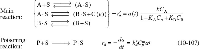
the surface sites would change with time as shown in Figure 10-27.

Progression of sites being poisoned
If we assume the rate of removal of the poison, rP⋅S, from the reactant gas stream onto the catalyst sites is proportional to the number of sites that are unpoisoned (Ct0 – CP·S) and the concentration of poison in the gas phase is CP then
rP·S = kd (Ct0 – CP·S)CP
where CP · S is the concentration of poisoned sites and Ct0 is the total number of sites initially available. Because every molecule that is adsorbed from the gas phase onto a site is assumed to poison the site, this rate is also equal to the rate of removal of total active sites (Ct) from the surface
Dividing through by Ct0 and letting f be the fraction of the total number of sites that have been poisoned yields
The fraction of sites available for adsorption (1 – f) is essentially the activity a(t). Consequently, Equation (10-108) becomes

A number of examples of catalysts with their corresponding catalyst poisons are given by Farrauto and Bartholomew.29
29 Ibid.
Packed-Bed Reactors. In packed-bed reactors where the poison is removed from the gas phase by being adsorbed on the specific catalytic sites, the deactivation process can move through the packed bed as a wave front. Here, at the start of the operation, only those sites near the entrance to the reactor will be deactivated because the poison (which is usually present in trace amounts) is removed from the gas phase by the adsorption; consequently, the catalyst sites farther down the reactor will not be affected. However, as time continues, the sites near the entrance of the reactor become saturated, and the poison must travel farther downstream before being adsorbed (removed) from the gas phase and attaching to a site to deactivate it. Figure 10-28 shows the corresponding activity profile for this type of poisoning process. We see in Figure 10-28 that by time t4 the entire bed has become deactivated. The corresponding overall conversion at the exit of the reactor might vary with time as shown in Figure 10-29.


The partial differential equations that describe the movement of the reaction front shown in Figure 10-28 are derived and solved in an example on the CRE Web site, at the very end of the Summary Notes for Chapter 10.
Poisoning by Either Reactants or Products. For the case where the main reactant also acts as a poison, the rate laws are

An example where one of the reactants acts as a poison is in the reaction of CO and H2 over ruthenium to form methane, with
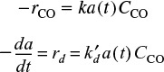
Similar rate laws can be written for the case when the product B acts as a poison.
For separable deactivation kinetics resulting from contacting a poison at a constant concentration CP0 and no spatial variation

Separable deactivation kinetics
The solution to this equation for the case of first-order decay, n = 1
is
Empirical Decay Laws. Table 10-7 gives a number of empirical decay laws along with the reaction systems to which they apply.
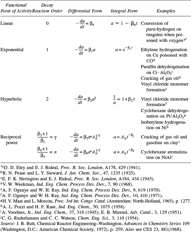
Examples of reactions with decaying catalysts and their decay laws
One should also see Fundamentals of Industrial Catalytic Processes, by Farrauto and Bartholomew, which contains rate laws similar to those in Table 10-7, and also gives a comprehensive treatment of catalyst deactivation.30
30 Ibid.
Key resource for catalyst deactivation
10.7.2 Reactors That Can Be Used to Help Offset Catalyst Decay
We will now consider three reaction systems that can be used to handle systems with decaying catalyst. We will classify these systems as those having slow, moderate, and rapid losses of catalytic activity. To offset the decline in chemical reactivity of decaying catalysts in continuous-flow reactors, the following three methods are commonly used:
• Slow decay – Temperature–Time Trajectories (10.7.3)
• Moderate decay – Moving-Bed Reactors (10.7.4)
• Rapid decay – Straight-Through Transport Reactors (10.7.5)
Matching the reactor type with speed of catalyst decay
10.7.3 Temperature–Time Trajectories
In many large-scale reactors, such as those used for hydrotreating, and reaction systems where deactivation by poisoning occurs, the catalyst decay is relatively slow. In these continuous flow systems, constant conversion is usually necessary in order that subsequent processing steps (e.g., separation) are not upset. One way to maintain a constant conversion with a decaying catalyst in a packed or fluidized bed is to increase the reaction rate by steadily increasing the feed temperature to the reactor. Operation of a “fluidized” bed in this manner is shown in Figure 10-30.
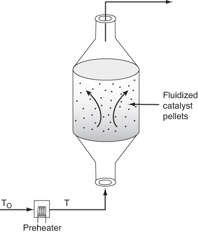
We are going to increase the feed temperature in such a manner that the reaction rate remains constant with time:
For a first-order reaction we have
k(T0)CA = a(t, T)k(T)CA
We will neglect any variations in concentration so that the product of the activity (a) and specific reaction rate (k) is constant and equal to the specific reaction rate, k0 at time t = 0 and temperature T0; that is
Slow rate of catalyst decay
The goal is to find how the temperature should be increased with time (i.e., the temperature–time trajectory) to maintain constant conversion. Using the Arrhenius equation to substitute for k in terms of the activation energy, EA, gives
Solving for 1/T yields

Gradually raising the temperature can help offset effects of catalyst decay.
The decay law also follows an Arrhenius-type temperature dependence

Substituting Equation (10-115) into (10-116) and rearranging yields

Integrating with a = 1 at t = 0 for the case n ≠ (1 + Ed/EA), we obtain

Solving Equation (10-114) for a and substituting in (10-118) gives

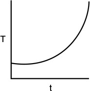
Equation (10-119) tells us how the temperature of the catalytic reactor should be increased with time in order for the reaction rate to remain constant.
In many industrial reactions, the decay rate law changes as temperature increases. In hydrocracking, the temperature–time trajectories are divided into three regimes. Initially, there is fouling of the acidic sites of the catalyst followed by a linear regime due to slow coking and, finally, accelerated coking characterized by an exponential increase in temperature. The temperature–time trajectory for a deactivating hydrocracking catalyst is shown in Figure 10-31.
Comparing theory and experiment

Figure 10-31 Temperature–time trajectories for deactivating hydrocracking catalyst, runs 3 and 4. (Krishnaswamy, S., and J. R. Kittrell. Analysis of Temperature–Time Data for Deactivating Catalysts. Industry and Engineering Chemistry Process Design and Development, 1979, 18(3), 399–403. Copyright © 1979, American Chemical Society. Reprinted by permission.)
For a first-order decay, Krishnaswamy and Kittrell’s expression, Equation (10-119), for the temperature–time trajectory reduces to
10.7.4 Moving-Bed Reactors
Reaction systems with significant catalyst decay require the continual regeneration and/or replacement of the catalyst. Two types of reactors currently in commercial use that accommodate production with decaying catalysts are the moving-bed and straight-through transport reactor. A schematic diagram of a moving-bed reactor (used for catalytic cracking) is shown in Figure 10-32.
The freshly regenerated catalyst enters the top of the reactor and then moves through the reactor as a compact packed bed. The catalyst is coked continually as it moves through the reactor until it exits the reactor into the kiln, where air is used to burn off the carbon. The regenerated catalyst is lifted from the kiln by an airstream and then fed into a separator before it is returned to the reactor. The catalyst pellets are typically between one-quarter and one-eighth in. in diameter.
The reactant feed stream enters at the top of the reactor and flows rapidly through the reactor relative to the flow of the catalyst through the reactor (Figure 10-33). If the feed rates of the catalyst and the reactants do not vary with time, the reactor operates at steady state; that is, conditions at any point in the reactor do not change with time. The mole balance on reactant A over ΔW is
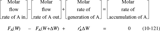

Figure 10-32 Thermofor catalytic cracking (TCC) unit. (Weekman, V. AIChE Monogr. Ser., 75(11), 4 (1979). With permission of the American Institute of Chemical Engineers. Copyright © 1979 AIChE. All rights reserved.)
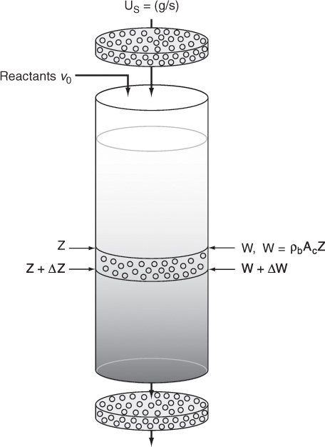
Figure 10-33 Moving-bed reactor schematic. The value of the catalyst contained in a reactor of this type is approximately $1 million.
Moving bed reactor, used for reactions with moderate rate of catalyst decay
Dividing by ΔW, letting ΔW approach zero, and expressing the flow rate in terms of conversion gives
Mole Balance
The rate of reaction at any time t is
The activity, as before, is a function of the time the catalyst has been in contact with the reacting gas stream. The decay rate law is
Decay Law
We now need to relate the contact time to the weight of the catalyst. Consider a point z in the reactor, where the reactant gas has passed cocurrently through a catalyst weight W. Because the solid catalyst is moving through the bed at a rate Us (mass per unit time), the time t that the catalyst has been in contact with the gas when the catalyst reaches a point z is
If we now differentiate Equation (10-122)
and combine it with the decay rate law, we obtain
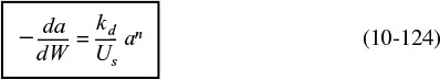
The activity equation is combined with the mole balance
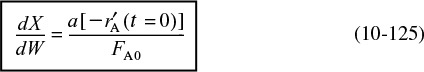
The design equation for moving-bed reactors
these two coupled differential equations (i.e., Equations (10-124) and (10-125)) are numerically solved simultaneously with an ODE solver, e.g., Polymath.
Example 10–5 Catalytic Cracking in a Moving-Bed Reactor
The catalytic cracking of a gas-oil charge, A, to form C5+ (B) and to form coke and dry gas (C) is to be carried out in a screw-type conveyor, moving-bed reactor at 900°F:

This cracking of gas oil can also be written as
While pure hydrocarbons are known to crack according to a first-order rate law, the fact that the gas-oil exhibits a wide spectrum of cracking rates gives rise to the fact that the lumped cracking rate is well represented by a second-order rate law (see Web Problem CDP5-HB) with the following specific reaction rate:31
31 Estimated from V. W. Weekman and D. M. Nace, AIChE J., 16, 397 (1970).
The catalytic deactivation is independent of gas-phase concentration and follows a first-order decay rate law, with a decay constant, kd of 0.72 reciprocal minutes. The feed stream is diluted with nitrogen so that as a first approximation, volume changes can be neglected with reaction. The reactor contains 22 kg of catalyst that moves through the reactor at a rate of 10 kg/min. The gas-oil is fed at a rate of 30 mol/min at a concentration of 0.075 mol/dm3. Determine the conversion that can be achieved in this reactor.
Solution
1. Mole Balance:
2. Rate Law:
3. Decay Law. First-order decay
Using Equation (10-124), we obtain
Integrating
Moving beds: moderate rate of catalyst decay
4. Stoichiometry. If υ ≈ υ0, then
5. Combining we have

The polymath program is shown below along with a conversion profile.
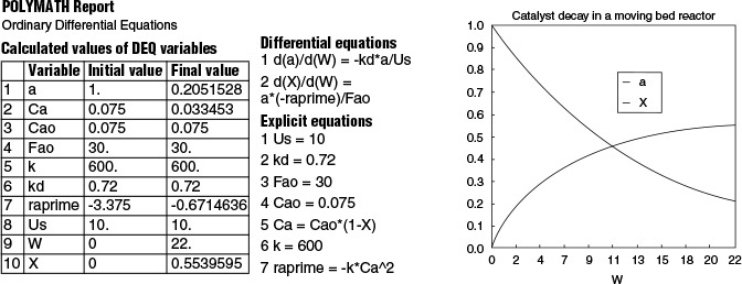
For the simple rate law and activity law given here, we also could have solved this problem analytically.
6. Separating and integrating yields

7. Numerical evaluation:

If there were no catalyst decay, the conversion would be
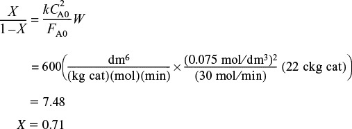
Analysis: The purpose of this example was to show step-by-step how to apply the algorithm to a moving-bed reactor that has been used to reduce the effects of catalyst decay that would occur in a PBR.
We will now rearrange Equation (E10-5.8) to a form more commonly found in the literature. Let λ be a dimensionless decay time
and Da2 be the Damköhler number for a second-order reaction (a reaction rate divided by a transport rate) for a packed-bed reactor
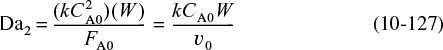
Through a series of manipulations we arrive at the equation for the conversion in a moving bed where a second-order reaction is taking place32
32 Ibid.

Second-order reaction in a moving-bed reactor
Similar equations are given or can easily be obtained for other reaction orders or decay laws.
10.7.5 Straight-Through Transport Reactors (STTR)
This reactor is used for reaction systems in which the catalyst deactivates very rapidly. Commercially, the STTR is used in the production of gasoline from the cracking of heavier petroleum fractions where coking of the catalyst pellets occurs very rapidly. In the STTR, the catalyst pellets and the reactant feed enter together and are transported very rapidly through the reactor. The bulk density of the catalyst particle in the STTR is significantly smaller than in moving-bed reactors, and often the particles are carried through at the same velocity as the gas velocity. In some places the STTR is also referred to as a circulating fluidized bed (CFB). A schematic diagram is shown in Figure 10-34.
A mole balance on the reactant A over the differential reactor volume
ΔV = AC Δz
is

STTR: Used when catalyst decay (usually coking) is very rapid
Dividing by Δz and taking the limit as Δz → 0 and recalling that ![]() , we obtain
, we obtain
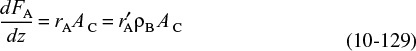
In terms of conversion and catalyst activity
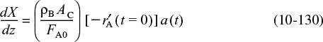
For a catalyst particle traveling through the reactor with a particle velocity UP, the time the catalyst pellet has been in the reactor when it reaches a height z is just
Substituting for time t in terms of distance z [i.e., a(t) = a(z/UP)], the mole balance now becomes
The entering molar flow rate, FA0, can be expressed in terms of the gas velocity Ug, CA0, and AC
FA0 = UoACCA0
Substituting for FA0, we have
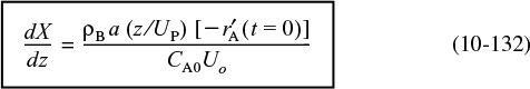
Example 10–6 Decay in a Straight-Through Transport Reactor
The vapor-phase cracking of a gas-oil is to be carried out in a straight-through transport reactor (STTR) that is 10-m high and 1.5 m in diameter. Gas-oil is a mixture of normal and branched paraffins (C12–C40), naphthenes, and aromatics, all of which will be lumped as a single species, A. We shall lump the primary hydrocarbon products according to distillate temperature into two respective groups, dry gas (C–C4) B and gasoline (C5–C14) C. The reaction
A typical cost of the catalyst in the reactor system is $1 million.
can be written symbolically as
Both B and C are adsorbed on the surface. The rate law for a gas-oil cracking reaction on fresh catalyst can be approximated by
with k′ = 0.0014 kmol/kg-cat·s·atm, KA = 0.05 atm–1, KB = 0.15 atm–1, and KC = 0.1 atm–1. The catalyst decays by the deposition of coke, which is produced in most cracking reactions along with the reaction products. The decay law is
Pure gas-oil enters at a pressure of 12 atm and a temperature of 400°C. The bulk density of catalyst in the STTR is 80 kg-cat/m3. Plot the activity and conversion of gas-oil up the reactor for entering gas velocity U0 = 2.5 m/s.
Solution
Mole Balance:

The height of the catalyst particle at time “t” after entering the STTR is
Differentiating, we can find a relation between the time the catalyst particle has been in the STTR and reached a height z, which we can use to find the activity a.
Rate Law:
On fresh catalyst
Combining Equations (E10-6.2) through (E10-6.4) gives

Decay Law. Assuming that the catalyst particle and gas travel up the reactor at the velocity UP = Ug = U, we obtain

where U = υ/AC = υ0 (1 + εX)/AC and AC = πD2/4.
Stoichiometry (gas-phase isothermal and no pressure drop):

Parameter Evaluation:

Equations (E10-6.1), (E10-6.5), (E10-6.7), and (E10-6.8) through (E10-6.10) are now combined and solved using an ODE solver. The Polymath program is shown in Table E10-6.1, and the computer output is shown in Figure E10-6.1.
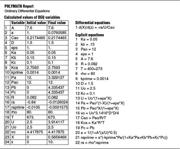
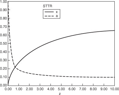
Analysis: In this example we applied the algorithm to a STTR in which the gas velocity and, hence, particle velocity increases as we move through the reactor. The decay is quite rapid and the activity is only 15% of its initial value at z = 3 m into the reactor and the conversion begins to plateau at z = 6 m at 60% conversion. If there were no catalyst decay (a = 0) the conversion would have been 97%.
a. Chemisorption
b. Physical adsorption
2. The Langmuir isotherm relating the concentration of species A on the surface to the partial pressure of A in the gas phase is
3. The sequence of steps for the solid-catalyzed isomerization
is:
a. Mass transfer of A from the bulk fluid to the external surface of the pellet
b. Diffusion of A into the interior of the pellet
c. Adsorption of A onto the catalytic surface
d. Surface reaction of A to form B
e. Desorption of B from the surface
f. Diffusion of B from the pellet interior to the external surface
g. Mass transfer of B away from the solid surface to the bulk fluid
4. Assuming that mass transfer is not rate-limiting, the rate of adsorption is

The rate of surface reaction is
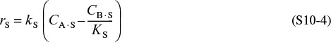
The rate of desorption is
At steady state
If there are no inhibitors present, the total concentration of sites is
5. If we assume that the surface reaction is rate-limiting, we set
and solve for CA·S and CB·S in terms of PA and PB. After substitution of these quantities in Equation (S10-4), the concentration of vacant sites is eliminated with the aid of Equation (S10-7)
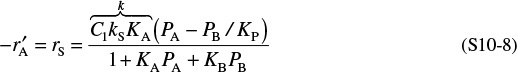
Recall that the equilibrium constant for desorption of species B is the reciprocal of the equilibrium constant for the adsorption of species B
and the thermodynamic equilibrium constant, KP, is
6. Chemical vapor deposition

7. Catalyst deactivation. The catalyst activity is defined as
The rate of reaction at any time t is
The rate of catalyst decay is
For first-order decay
For second-order decay
8. For slow catalyst decay, the idea of a temperature–time trajectory is to increase the temperature in such a way that the rate of reaction remains constant.
9. The coupled differential equations to be solved for a moving-bed reactor are
For nth-order activity decay and m order in a gas-phase concentration of species i
10. The coupled differential equations to be solved in a straight-through transport reactor for the case when the particle and gas velocities, U, are identical are
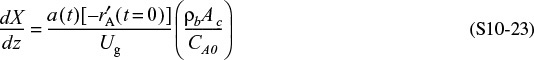
For coking
Ode Solver Algorithm
The isomerization A → B is carried out over a decaying catalyst in a moving-bed reactor. Pure A enters the reactor and the catalyst flows through the reactor at a rate of 2.0 kg/s.

1. Puzzle Problem “What’s Wrong with this Solution?”
2. Turn Over Frequency (TOF)
3. Algorithm When More than One of the Three Steps in a Catalytic Reaction Mechanism (Adsorption, Surface Reaction, Desorption) Is Rate Limiting
4. Additional Homework Problems
• Learning Resources
1. Summary Notes for Chapter 10
2. Interactive Computer Modules
A. Heterogeneous Catalysis
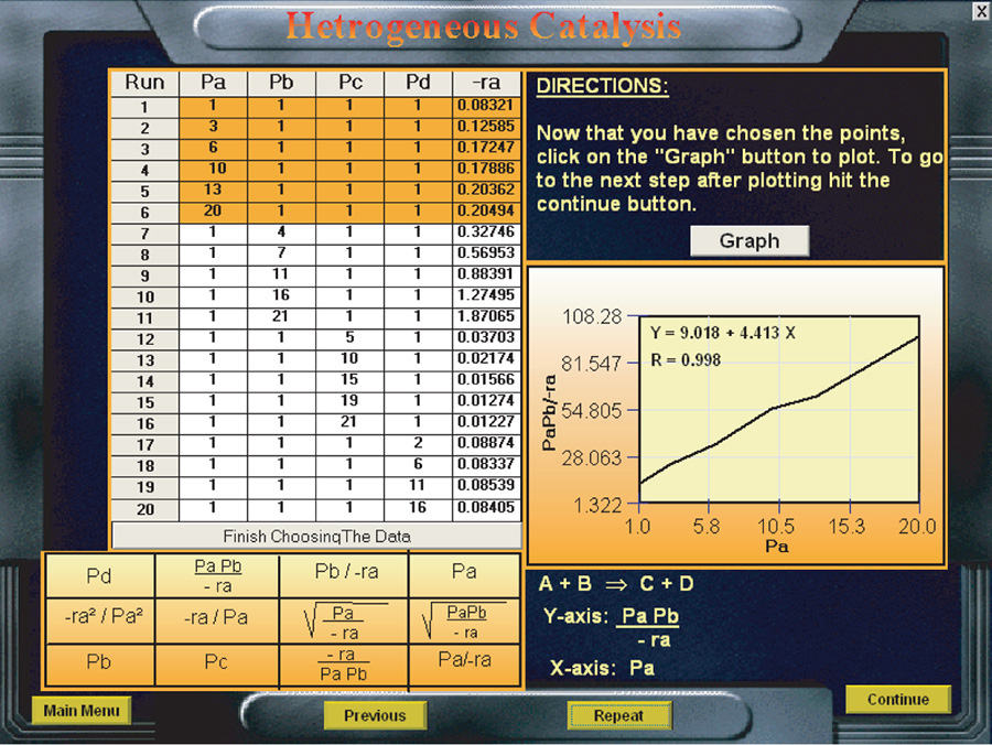
3. Solved Problems
Example Chapter 10 CRE Web Site: 10-1 Analysis of a Heterogeneous Reaction
[Class Problem University of Michigan]
Example Chapter 10 CRE Web Site: 10-2 Least Squares Analysis to Determine the
Rate Law Parameters k, kT, and kB
Example Chapter 10 CRE Web Site: 10-3 Decay in a Straight-Through Reactor
Example Chapter 10 CRE Web Site: 10-4 Catalyst Poisoning in a Batch Reactor

• Living Example Problems
1. Example 10-2 Regression Analysis to Determine Model Parameters
2. Example 10-3 Fixed-Bed Reactor Design
3. Example 10-4 Model Discrimination
4. Example 10-5 Catalyst Decay in a Batch Reactor
5. Example 10-6 Catalyst Decay in a Fluidized Bed Modeled as a CSTR
6. Example 10-8 Decay in a Straight-Through Transport Reactor
• Professional Reference Shelf
R10.1. Classification of Catalysts
R10.2. Hydrogen Adsorption
A. Molecular Adsorption
B. Dissociative Adsorption
R10.2. Analysis of Catalyst Decay Laws
A. Integral Method
B. Differential Method
R10.3. Etching of Semiconductors
A. Dry Etching
B. Wet Etching
C. Dissolution Catalysis
A. Type of Catalyst Deactivation
B. Temperature–Time Trajectories
C. Moving-Bed Reactors
D. Straight-Through Transport Reactors
After Reading Each Page in This Book, Ask Yourself a Question About What You Read
Questions and Problems
The subscript to each of the problem numbers indicates the level of difficulty: A, least difficult; D, most difficult.
Questions
Q10-1A Read over the problems at the end of this chapter. Make up an original problem that uses the concepts presented in this chapter. See Problem P5-1A for guidelines. To obtain a solution:
(a) Create your data and reaction.
(b) Use a real reaction and real data.
The journals listed at the end of Chapter 1 may be useful for part (b).
(c) Choose an FAQ from Chapter 10 and explain why it was most helpful.
(d) Listen to the audios ![]() on the Summary Notes, pick one, and explain why it was most helpful.
on the Summary Notes, pick one, and explain why it was most helpful.
(a) Example 10-1. Plot and analyze (1) the ratio of toluene-occupied sites to benzene-occupied sites, (2) the fraction of vacant sites, and (3) the fraction of benzene-occupied sites as a function of conversion at 1 atm.
(b) Example 10-2. (1) What if the entering pressure were increased to 80 atm or reduced 1 atm, how would your answers change? (2) What if the molar flow rate were reduced by 50%, how would X and y change? (3) What catalyst weight would be required for 60% conversion?
(c) Example 10-3. (1) How would your answers change if the following data for run 10 were incorporated in your regression table?
![]() = 0.8 mol/kg-cat ⋅ s, PE = 0.5 atm, PEA = 15 atm, PH = 2 atm.
= 0.8 mol/kg-cat ⋅ s, PE = 0.5 atm, PEA = 15 atm, PH = 2 atm.
(2) How do the rate laws (e) and (f)
compare with the other rate laws used to model the data?
(3) Write a question for this problem that involves critical thinking and explain why it involves critical thinking.
(d) Example 10-4. Vary k and kd, and describe what you find.
(e) Example 10-5. (1) Sketch X vs. t for various values of kd and k. Pay particular attention to the ratio k/kd. (2) Repeat (1) for this example (i.e., the plotting of X vs. t) for a second-order reaction with (CA0 = 1 mol/dm3) and first-order decay. (3) Repeat (2) for this example for a first-order reaction and first-order decay. (4) Repeat (1) for this example for a second-order reaction (CA0 = 1 mol/dm3) and a second-order decay.
(f) Example 10-7. (1) What if the solids and reactants entered from opposite ends of the reactor? How would your answers change? (2) What if the decay in the moving bed were second order? By how much must the catalyst charge, Us, be increased to obtain the same conversion? (3) What if ε = 2 (e.g., A → 3B) instead of zero, how would the results be affected?
(g) Example 10-8. (1) What if you varied the parameters PA0, Ug, A, and k′ in the STTR? What parameter has the greatest effect on either increasing or decreasing the conversion? Ask questions such as: What is the effect of varying the ratio of k to Ug or of k to A on the conversion? Make a plot of conversion versus distance as Ug is varied between 0.5 and 50 m/s. Sketch the activity and conversion profiles for Ug = 0.025, 0.25, 2.5, and 25 m/s. What generalizations can you make? Plot the exit conversion and activity as a function of gas velocity between velocities of 0.02 and 50 m/s. What gas velocity do you suggest operating at? What is the corresponding entering volumetric flow rate? What concerns do you have operating at the velocity you selected? Would you like to choose another velocity? If so, what is it?
(h) What if you were asked to sketch the temperature–time trajectories and to find the catalyst lifetimes for first- and for second-order decay when EA = 35 kcal/mol, Ed = 10 kcal/mol, kd0 = 0.01 day–1, and T0 = 400 K? How would the trajectory of the catalyst lifetime change if EA = 10 kcal/mol and Ed = 35 kcal/mol? At what values of kd0 and ratios of Ed to EA would temperature–time trajectories not be effective? What would your temperature–time trajectory look like if n = 1 + Ed/EA?
(i) Write a question for this problem that involves critical thinking and explain why it involves critical thinking.
P10-2A Download the Interactive Computer Games (ICG) from the CRE Web site. Play the game and then record your performance number for the game, which indicates your mastery of the material. Your professor has the key to decode your performance number. (This ICG is a little longer than the other ICGs.) ICG Heterogeneous Catalysis Performance # _________________.
P10-3A t-Butyl alcohol (TBA) is an important octane enhancer that is used to replace lead additives in gasoline [Ind. Eng. Chem. Res., 27, 2224 (1988)]. TBA was produced by the liquid-phase hydration (W) of isobutene (I) over an Amberlyst-15 catalyst. The system is normally a multiphase mixture of hydrocarbon, water, and solid catalysts. However, the use of cosolvents or excess TBA can achieve reasonable miscibility.
The reaction mechanism is believed to be

Derive a rate law assuming:
(a) The surface reaction is rate-limiting.
(b) The adsorption of isobutene is limiting.
(c) The reaction follows Eley–Rideal kinetics
and the surface reaction is limiting.
(d) Isobutene (I) and water (W) are adsorbed on different sites.
TBA is not on the surface, and the surface reaction is rate-limiting.

(e) What generalization can you make by comparing the rate laws derived in parts (a) through (d)?
P10-4B Consider the catalytic reaction as a function of the initial partial pressures
The rate of disappearance of species A was obtained in a differential reactor and is shown below.
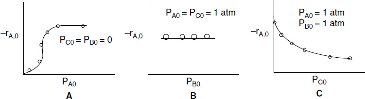
(a) What species are on the surface?
(b) What does Figure B tell you about the reversibility and what’s adsorbed on the surface?
(c) Derive the rate law and suggest a rate-liming step consistent with the above figures.
(d) How would you plot your data to linearize the initial rate data in Figure A?
(e) Assuming pure A is fed, and the adsorption constants for A and C are KA = 0.5 atm–1 and KC = 0.25 atm–1 respectively, at what conversion are the number of sites with A adsorbed on the surface and C adsorbed on the surface equal? (Ans.: X = 0.66)
P10-5A The rate law for the hydrogenation (H) of ethylene (E) to form ethane (A) over a cobalt-molybdenum catalyst [Collection Czech. Chem. Commun., 51, 2760 (1988)] is
(a) Suggest a mechanism and rate-limiting step consistent with the above rate law.
(b) What was the most difficult part in finding the mechanism?
P10-6B The formation of propanol on a catalytic surface is believed to proceed by the following mechanism

Suggest a rate-limiting step and derive a rate law.
P10-7B The dehydration of n-butyl alcohol (butanol) over an alumina-silica catalyst was investigated by J. F. Maurer (Ph.D. thesis, University of Michigan). The data in Figure P10-7B were obtained at 750°F in a modified differential reactor. The feed consisted of pure butanol.
(a) Suggest a mechanism and rate-limiting step that are consistent with the experimental data.
(b) Evaluate the rate-law parameters.
(c) At the point where the initial rate is a maximum, what is the fraction of vacant sites? What is the fraction of occupied sites by both A and B? % vacant = 0.41
(d) What generalizations can you make from studying this problem?
(e) Write a question that requires critical thinking and then explain why your question requires critical thinking. Hint: See Preface Section I.
(f) Apply one or more of the six ideas in Preface Table P-4, page xxviii, to this problem.

P10-8B The catalytic dehydration of methanol (ME) to form dimethyl ether (DME) and water was carried out over an ion exchange catalyst [K. Klusacek, Collection Czech. Chem. Commun., 49, 170 (1984)]. The packed bed was initially filled with nitrogen, and at t = 0. The N2 feed is switched to pure methanol vapor entering the reactor at 413 K, 100 kPa, and 0.2 cm3/s. The following partial pressures were recorded at the exit to the differential reactor containing 1.0 g of catalyst in 4.5 cm3 of reactor volume.


Use parts (a) through (f) to lead you to suggest a mechanism, rate-limiting step, and rate law consistent with this data.
(a) Using the data above, sketch the exit concentrations as a function of time.
(b) Which species took longer than others to exit the reactor in the gas phase? What could have caused this difference in exit times?
(c) What species are adsorbed on the surface?
(d) Are any species not adsorbed on the surface? If so, which ones?
(e) Which set of figures, (1)-(4) below, correctly describes the functionality of the chemical reaction rate with the partial pressures PW, PDME, and PME?
(f) Derive a rate law for the catalytic dehydration of methanol. Dimethyl Either 2ME → DME + W.

P10-9B In 1981, the U.S. government put forth the following plan for automobile manufacturers to reduce emissions from automobiles over the next few years.
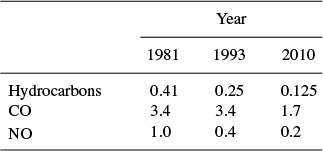
All values are in grams per mile. An automobile emitting 3.74 lbm of CO and 0.37 lbm of NO on a journey of 1000 miles would meet the current government requirements.

To remove oxides of nitrogen (assumed to be NO) from automobile exhaust, a scheme has been proposed that uses unburned carbon monoxide (CO) in the exhaust to reduce the NO over a solid catalyst, according to the reaction
Experimental data for a particular solid catalyst indicate that the reaction rate can be well represented over a large range of temperatures by

(a) Propose an adsorption–surface reaction–desorption mechanism and rate-limiting step that are consistent with the experimentally observed rate law. Do you need to assume any species are weakly adsorbed to get agreement with Equation (P10-9.1)?
(b) A certain engineer thinks that it would be desirable to operate with a very large stoichiometric excess of CO to minimize catalytic reactor volume. Do you agree or disagree? Explain.
(c) What would be the relevance of the problem if everyone were driving a hybrid by 2018? A driverless car by 2020?
P10-10B Methyl ethyl ketone (MEK) is an important industrial solvent that can be produced from the dehydrogenation of butan-2-ol (Bu) over a zinc oxide catalyst [Ind. Eng. Chem. Res., 27, 2050 (1988)]:
The following data giving the reaction rate for MEK were obtained in a differential reactor at 490°C.

(a) Suggest a rate law consistent with the experimental data.
(b) Suggest a reaction mechanism and rate-limiting step consistent with the rate law. Hint: Some species might be weakly adsorbed.
(c) Apply one or more of the six ideas in Preface Table P-4, page xxviii, to this problem.
(d) Plot conversion (up to 90%) and reaction rate as a function of catalyst weight for an entering molar flow rate of pure butan-2-ol of 10 mol/min at an entering pressure P0 = 10 atm up to a catalyst weight Wmax = 23 kg.
(e) Write a question that requires critical thinking and then explain why your question requires critical thinking. Hint: See Preface Section I.
(f) Repeat part (d), accounting for pressure drop and α = 0.03 kg–1. Plot p and X as a function of catalyst weight down the reactor.
P10-11B Cyclohexanol was passed over a catalyst to form water and cyclohexene:
It is suspected that the reaction may involve a dual-site mechanism, but it is not known for certain. It is believed that the adsorption equilibrium constant for cyclohexanol is around 1.0 and is roughly one or two orders of magnitude greater than the adsorption equilibrium constants for the other compounds. Using these data:
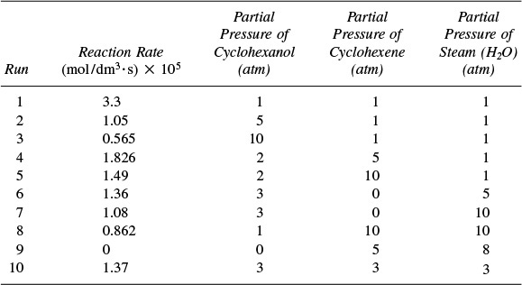
(a) Suggest a rate law and mechanism consistent with the data given here.
(b) Determine the values of the rate-law parameters. (Ind. Eng. Chem. Res., 32, 2626–2632.)
(c) Why do you think estimates of the rate-law parameters were given?
(d) For an entering molar flow rate of cychlohexanol of 10 mol/s at a partial pressure of 15 atm, what catalyst weight is necessary to achieve 85% conversion when the bulk density is 1500 gm/dm3?
P10-12B Experimental data for the gas-phase catalytic reaction
A + B → C
is shown below. The limiting step in the reaction is known to be irreversible, so that the overall reaction is irreversible. The reaction was carried out in a differential reactor to which A, B, and C were all fed.

(a) Suggest a rate law consistent with the experimental data. Hint: Sketch (![]() ) as a function of PA, as a function of PB, and as a function of PC.
) as a function of PA, as a function of PB, and as a function of PC.
(b) From your rate expression, which species can you conclude are adsorbed on the surface?
(c) Suggest a rate law and then show that your mechanism is constant with the rate law in part (a).
(d) For an entering partial pressure of A of 2 atm in a PBR, what is the ratio of A to C sites at 80% conversion of A?
(e) At what conversion are the number of A and C sites equal? (Ans.: X = 0.235)
(f) What catalyst weight is necessary to achieve 90% conversion of A for a stoichiometric feed and flow of A 2 mol/s? (Ans.: W = 8.9 g-cat)
If necessary, feel free to use none, any, or all of the following parameter values:
P10-13B Solar Energy Capture: Water Splitting. Hydrogen and O2 can be combined in fuel cells to generate electricity. Solar energy can be used to split water to generate the raw reactants H2 and O2 for fuel cells. One method of solar thermal reduction is with NiFe2O4 in the sequence

We note NiFe2O4 is regenerated in this process.33
33 Scheffe, J.R., J. Li, and A. W. Weimer, “A Spinel Ferrite/Hercynite Water-Splitting Redox Cycle,” International Journal of Hydrogen Energy, 35, 3333–3340 (2010).
(a) Derive a rate law for Step (2), assuming that water adsorbs on the solid solution as a single-site mechanism and that the reaction is irreversible.
(b) Repeat (a) when the reaction is reversible and the solid solution adsorption site for water (S′) is different than the NiFe2O4 site for the adsorption of H2, (S).

(c) How would your rate law change if we included Step 1?
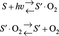
P10-14A Vanadium oxides are of interest for various sensor applications, owing to the sharp metal–insulator transitions they undergo as a function of temperature, pressure, or stress. Vanadium triisopropoxide (VTIPO) was used to grow vanadium oxide films by chemical vapor deposition [J. Electrochem. Soc., 136, 897 (1989)]. The deposition rate as a function of VTIPO pressure for two different temperatures follows.
T = 120°C:
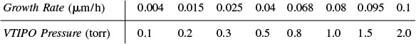
T = 200°C:
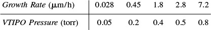
In light of the material presented in this chapter, analyze the data and describe your results. Specify where additional data should be taken.
P10-15A Titanium dioxide is a wide-bandgap semiconductor that is showing promise as an insulating dielectric in VLSI capacitors and for use in solar cells. Thin films of TiO2 are to be prepared by chemical vapor deposition from gaseous titanium tetraisopropoxide (TTIP). The overall reaction is
The reaction mechanism in a CVD reactor is believed to be [K. L. Siefering and G. L. Griffin, J. Electrochem. Soc., 137, 814 (1990)]
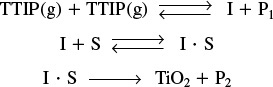
where I is an active intermediate and P1 is one set of reaction products (e.g., H2O, C3H6), and P2 is another set. Assuming the homogeneous gas-phase reaction for TTIP is in equilibrium, derive a rate law for the deposition of TiO2. The experimental results show that at 200°C the reaction is second order at low partial pressures of TTIP and zero order at high partial pressures, while at 300°C the reaction is second order in TTIP over the entire pressure range. Discuss these results in light of the rate law you derived.
P10-16B The dehydrogenation of methylcyclohexane (M) to produce toluene (T) was carried out over a 0.3% Pt/Al2O3 catalyst in a differential catalytic reactor. The reaction is carried out in the presence of hydrogen (H2) to avoid coking [J. Phys. Chem., 64, 1559 (1960)].
(a) Determine the model parameters for each of the following rate laws.
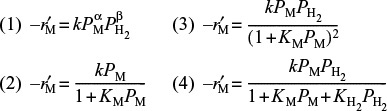
Use the data in Table P10-16B below.
(b) Which rate law best describes the data? Hint: Neither KH2 or KM can take on negative values.
(c) Where would you place additional data points?
(d) Suggest a mechanism and rate-limiting step consistent with the rate law you have chosen.

P10-17A Sketch qualitatively the reactant, product, and activity profiles as a function of length at various times for a packed-bed reactor for each of the following cases. In addition, sketch the effluent concentration of A as a function of time. The reaction is a simple isomerization:
(a)
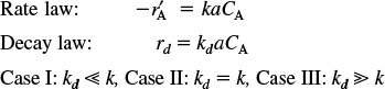
(b) ![]() = kaCA and rd = kd a2
= kaCA and rd = kd a2
(c) ![]() = kaCA and rd = kd aCB
= kaCA and rd = kd aCB
(d) Sketch similar profiles for the rate laws in parts (a) and (c) in a moving-bed reactor with the solids entering at the same end of the reactor as the reactant.
(e) Repeat part (d) for the case where the solids and the reactant enter at opposite ends.
P10-18B The elementary irreversible gas-phase catalytic reaction
is to be carried out in a moving-bed reactor at constant temperature. The reactor contains 5 kg of catalyst. The feed is stoichiometric in A and B. The entering concentration of A is 0.2 mol/dm3. The catalyst decay law is zero order with kD = 0.2 s–1 and k = 1.0 dm6/(mol ⋅ kg-cat ⋅ s) and the volumetric flow rate is υ0 = 1 dm3/s.
(a) What conversion will be achieved for a catalyst feed rate of 0.5 kg/s? (Ans.: X = 0.2)
(b) Sketch the catalyst activity as a function of catalyst weight (i.e., distance) down the reactor length for a catalyst feed rate of 0.5 kg/s.
(c) What is the maximum conversion that could be achieved (i.e., at an infinite catalyst loading rate)?
(d) What catalyst loading rate is necessary to achieve 40% conversion? (Ans.: US = 1.5 kg/s)
(e) At what catalyst loading rate (kg/s) will the catalyst activity be exactly zero at the exit of the reactor?
(f) What does an activity of zero mean? Can catalyst activity be less than zero?
(g) How would your answer in part (a) change if the catalyst and reactant were fed at opposite ends? Compare with part (a).
(h) Now consider the reaction to be zero order with
k = 0.2 mol/kg-cat ⋅ min.
The economics:
• The product sells for $160 per gram mole.
• The cost of operating the bed is $10 per kilogram of catalyst exiting the bed.
What is the feed rate of solids (kg/min) that will give the maximum profit? (Ans.: Us = 4 kg/min.) (Note: For the purpose of this calculation, ignore all other costs, such as the cost of the reactant, the cost to the company of providing free lunches to workers, etc.)
P10-19B With the increasing demand for xylene in the petrochemical industry, the production of xylene from toluene disproportionation has gained attention in recent years [Ind. Eng. Chem. Res., 26, 1854 (1987)]. This reaction,

was studied over a hydrogen mordenite catalyst that decays with time. As a first approximation, assume that the catalyst follows second-order decay
rd = kda2
and the rate law for low conversions is
with kT = 20 g mol/h ·kg-cat ·atm and kd = 1.6 h–1 at 735 K.
(a) Compare the conversion-time curves in a batch reactor containing 5 kg-cat at different initial partial pressures (1 atm, 10 atm, etc.). The reaction volume containing pure toluene initially is 1 dm3 and the temperature is 735 K.
(b) What conversion can be achieved in a moving-bed reactor containing 50 kg of catalyst with a catalyst feed rate of 2 kg/h? Toluene is fed at a pressure of 2 atm and a rate of 10 mol/min.
(c) Explore the effect of catalyst feed rate on conversion.
(d) Suppose that ET = 25 kcal/mol and Ed = 10 kcal/mol. What would the temperature–time trajectory look like for a CSTR? What if ET = 10 kcal/mol and Ed = 25 kcal/mol?
(e) The decay law more closely follows the equation
with kd = 0.2 atm–2 h–1. Redo parts (b) and (c) for these conditions.
P10-20A The vapor-phase cracking of gas-oil in Example 10-6 is carried out over a different catalyst, for which the rate law is
(a) Assuming that you can vary the entering pressure and gas velocity, what operating conditions would you recommend?
(b) What could go wrong with the conditions you chose?
Now assume the decay law is
where the concentration, Ccoke, in mol/dm3, can be determined from a stoichiometric table.
(c) For a temperature of 400°C and a reactor height of 15 m, what gas velocity do you recommend? Explain. What is the corresponding conversion?
(d) The reaction is now to be carried in an STTR 15 m high and 1.5 m in diameter. The gas velocity is 2.5 m/s. You can operate in the temperature range between 100 and 500°C. What temperature do you choose, and what is the corresponding conversion?
(e) What would the temperature–time trajectory look like for a CSTR?
Additional information:
ER = 3000 cal/mol
ED = 15,000 cal/mol
P10-21C When the impurity cumene hydroperoxide is present in trace amounts in a cumene feed stream, it can deactivate the silica-alumina catalyst over which cumene is being cracked to form benzene and propylene. The following data were taken at 1 atm and 420°C in a differential reactor. The feed consists of cumene and a trace (0.08 mol %) of cumene hydroperoxide (CHP).
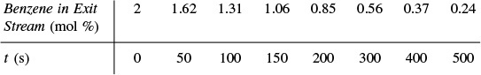
(a) Determine the order of decay and the decay constant. (Ans.: kd = 4.27 × 10⁻³ s–1.)
(b) As a first approximation (actually a rather good one), we shall neglect the denominator of the catalytic rate law and consider the reaction to be first order in cumene. Given that the specific reaction rate with respect to cumene is k = 3.8 × 10³ mol/kg fresh cat · s ·atm, the molar flow rate of cumene (99.92% cumene, 0.08% CHP) is 200 mol/min, the entering concentration is 0.06 kmol/m3, the catalyst weight is 100 kg, and the velocity of solids is 1.0 kg/min, what conversion of cumene will be achieved in a moving-bed reactor?
P10-22C The decomposition of spartanol to wulfrene and CO2 is often carried out at high temperatures [J. Theor. Exp., 15, 15 (2014)]. Consequently, the denominator of the catalytic rate law is easily approximated as unity, and the reaction is first order with an activation energy of 150 kJ/mol. Fortunately, the reaction is irreversible. Unfortunately, the catalyst over which the reaction occurs decays with time on stream. The following conversion-time data were obtained in a differential reactor:
For T = 500 K:

For T = 550 K:

(a) If the initial temperature of the catalyst is 480 K, determine the temperature–time trajectory to maintain a constant conversion.
(b) What is the catalyst lifetime?
P10-23B The hydrogenation of ethylbenzene to ethylcyclohexane over a nickel-mordenite catalyst is zero order in both reactants up to an ethylbenzene conversion of 75% [Ind. Eng. Chem. Res., 28 (3), 260 (1989)]. At 553 K, k = 5.8 mol ethylbenzene/(dm3 of catalyst ·h). When a 100-ppm thiophene concentration entered the system, the ethylbenzene conversion began to drop.
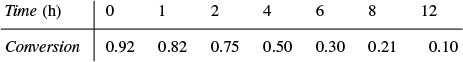
The reaction was carried out at 3 MPa and a molar ratio of H2/ETB = 10. Discuss the catalyst decay. Be quantitative where possible.
Supplementary Reading
1. A terrific discussion of heterogeneous catalytic mechanisms and rate-controlling steps may or may not be found in
BURGESS, THORNTON W., The Adventures of Grandfather Frog. New York: Dover Publications, Inc., 1915.
MASEL, R. I., Principles of Adsorption and Reaction on Solid Surfaces. New York: Wiley, 1996. A great reference.
SOMORJAI, G. A., Introduction to Surface Chemistry and Catalysis. New York: Wiley, 1994.
2. A truly excellent discussion of the types and rates of adsorption together with techniques used in measuring catalytic surface areas is presented in
MASEL, R. I., Principles of Adsorption and Reaction on Solid Surfaces. New York: Wiley, 1996.
3. Techniques for discriminating between mechanisms and models can be found in
BOX, G. E. P., W. G. HUNTER, and J. S. HUNTER, Statistics for Experimenters. New York: Wiley, 1978.
4. Examples of applications of catalytic principles to microelectronic manufacturing can be found in
BUTT, JOHN B, Reaction Kinetics and Reactor Design. Second Edition, Revised and Expanded. New York: Marcel Dekker, Inc., 1999.
DOBKIN, D. M., and M. K. ZURAW. Principles of Chemical Vapor Deposition. The Netherlands: Kluwer Academic Publishers, 2003.