11. Nonisothermal Reactor Design—The Steady-State Energy Balance and Adiabatic PFR Applications
If you can’t stand the heat, get out of the kitchen.
—Harry S Truman
11.1 Rationale
To identify the additional information necessary to design nonisothermal reactors, we consider the following example, in which a highly exothermic reaction is carried out adiabatically in a plug-flow reactor.
Example 11–1 What Additional Information Is Required?
The first-order liquid-phase reaction
is carried out in a PFR. The reaction is exothermic and the reactor is operated adiabatically. As a result, the temperature will increase with conversion down the length of the reactor. Because T varies along the length of the reactor, k will also vary, which was not the case for isothermal plug-flow reactors.

Calculate the PFR reactor volume necessary for 70% conversion and plot the corresponding profiles for X and T.
Solution
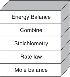
The same CRE algorithm can be applied to nonisothermal reactions as to isothermal reactions by adding one more step, the energy balance.
1. Mole Balance (design equation):
2. Rate Law:
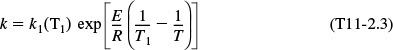
Recalling the Arrhenius equation,
we know that k is a function of temperature, T.

3. Stoichiometry (liquid phase): υ = υ0
4. Combining:

Combining Equations (E11-1.1), (E11-1.2), and (E11-1.4), and canceling the entering concentration, CA0, yields
Combining Equations (E11-1.3) and (E11-1.6) gives us
Why we need the energy balance
We see that we need another relationship relating X and T or T and V to solve this equation. The energy balance will provide us with this relationship.
So we add another step to our algorithm; this step is the energy balance.
5. Energy Balance:
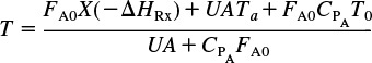
In this step, we will find the appropriate energy balance to relate temperature and conversion or reaction rate. For example, if the reaction is adiabatic, we will show that for equal heat capacities, CPA and CP, and a constant heat of reaction, ![]() , the temperature-conversion relationship can be written in a form such as
, the temperature-conversion relationship can be written in a form such as
T0 = Entering Temperature
ΔHRx = Heat of Reaction
CPA = Heat Capacity of species A
We now have all the equations we need to solve for the conversion and temperature profiles.
Analysis: The purpose of this example was to demonstrate that for nonisothermal chemical reactions we need another step in our CRE algorithm, the energy balance. The energy balance allows us to solve for the reaction temperature, which is necessary in evaluating the specific reaction rate constant k(T).
11.2 The Energy Balance
11.2.1 First Law of Thermodynamics
We begin with the application of the first law of thermodynamics, first to a closed system and then to an open system. A system is any bounded portion of the universe, moving or stationary, which is chosen for the application of the various thermodynamic equations. For a closed system, in which no mass crosses the system boundaries, the change in total energy of the system, dÊ, is equal to the heat flow to the system, δQ, minus the work done by the system on the surroundings, δW. For a closed system, the energy balance is
The δ’s signify that δQ and δW are not exact differentials of a state function.
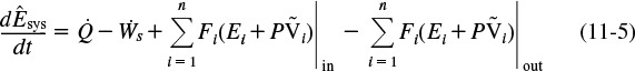
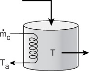
The continuous-flow reactors we have been discussing are open systems in which mass crosses the system boundary. We shall carry out an energy balance on the open system shown in Figure 11-1. For an open system in which some of the energy exchange is brought about by the flow of mass across the system boundaries, the energy balance for the case of only one species entering and leaving becomes

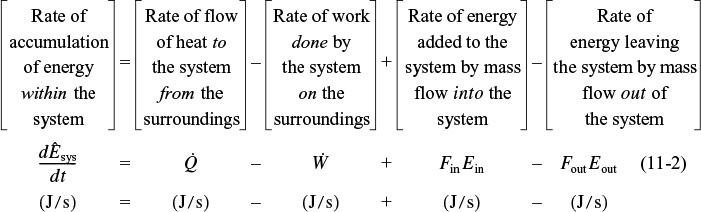
Energy balance on an open system
Typical units for each term in Equation (11-2) are (Joule/s).
We will assume that the contents of the system volume are well mixed, an assumption that we could relax but that would require a couple of pages of text to develop, and the end result would be the same! The unsteady-state energy balance for an open well-mixed system that has n species, each entering and leaving the system at its respective molar flow rate Fi (moles of i per time) and with its respective energy Ei (joules per mole of i), is

The starting point
We will now discuss each of the terms in Equation (11-3).
11.2.2 Evaluating the Work Term
It is customary to separate the work term, ![]() , into flow work and other work,
, into flow work and other work, ![]() . The term
. The term ![]() , often referred to as the shaft work, could be produced from such things as a stirrer in a CSTR or a turbine in a PFR. Flow work is work that is necessary to get the mass into and out of the system. For example, when shear stresses are absent, we write
, often referred to as the shaft work, could be produced from such things as a stirrer in a CSTR or a turbine in a PFR. Flow work is work that is necessary to get the mass into and out of the system. For example, when shear stresses are absent, we write

Flow work and shaft work
where P is the pressure (Pa) [1 Pa = 1 Newton/m2 = 1 kg·m/s2/m2] and ![]() is the specific molar volume of species i (m3/mol of i).
is the specific molar volume of species i (m3/mol of i).
Let’s look at the units of the flow-work term, which is
where Fi is in mol/s, P is Pa (1 Pa = 1 Newton/m2), and ![]() is m3/mol.
is m3/mol.

We see that the units for flow work are consistent with the other terms in Equation (11-3), i.e., J/s.
In most instances, the flow-work term is combined with those terms in the energy balance that represent the energy exchange by mass flow across the system boundaries. Substituting Equation (11-4) into (11-3) and grouping terms, we have
Convention
Heat Added![]()
Heat Removed![]()
Work Done by System![]()
Work Done on System![]()
The energy Ei is the sum of the internal energy (Ui), the kinetic energy (![]() ), the potential energy (gzi), and any other energies, such as electric or magnetic energy or light
), the potential energy (gzi), and any other energies, such as electric or magnetic energy or light
In almost all chemical reactor situations, the kinetic, potential, and “other” energy terms are negligible in comparison with the enthalpy, heat transfer, and work terms, and hence will be omitted; that is
We recall that the enthalpy, Hi (J/mol), is defined in terms of the internal energy Ui (J/mol), and the product P![]() (1 Pa·m3/mol = 1 J/mol):
(1 Pa·m3/mol = 1 J/mol):
Enthalpy
Typical units of Hi are
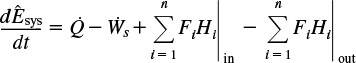
Enthalpy carried into (or out of) the system can be expressed as the sum of the internal energy carried into (or out of) the system by mass flow plus the flow work:
Combining Equations (11-5), (11-7), and (11-8), we can now write the energy balance in the form
The energy of the system at any instant in time, Êsys, is the sum of the products of the number of moles of each species in the system multiplied by their respective energies. This term will be discussed in more detail when unsteady-state reactor operation is considered in Chapter 13.
We shall let the subscript “0” represent the inlet conditions. Unsubscripted variables represent the conditions at the outlet of the chosen system volume.
Energy Balance

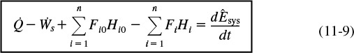
In Section 11.1, we discussed that in order to solve reaction engineering problems with heat effects, we needed to relate temperature, conversion, and rate of reaction. The energy balance as given in Equation (11-9) is the most convenient starting point as we proceed to develop this relationship.
11.2.3 Overview of Energy Balances
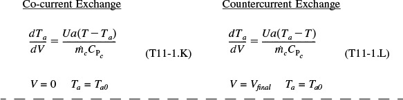
What is the plan? In the following pages we manipulate Equation (11-9) in order to apply it to each of the reactor types we have been discussing: batch, PFR, PBR, and CSTR. The end result of the application of the energy balance to each type of reactor is shown in Table 11-1. These equations can be used in Step 5 of the algorithm discussed in Example E11-1. The equations in Table 11-1 relate temperature to conversion and to molar flow rates, and to the system parameters, such as the overall heat-transfer coefficient and area, Ua, with the corresponding ambient temperature, Ta, and the heat of reaction, ΔHRx.
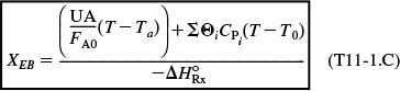
1. Adiabatic (![]() ) CSTR, PFR, Batch, or PBR. The relationship between conversion calculated from the energy balance, XEB, and temperature for
) CSTR, PFR, Batch, or PBR. The relationship between conversion calculated from the energy balance, XEB, and temperature for ![]() , constant CPi, and ΔCP = 0, is
, constant CPi, and ΔCP = 0, is
Conversion in terms of temperature

Temperature in terms of conversion calculated from the energy balance

End results of manipulating the energy balance (Sections 11.2.4, 12.1, and 12.3)
For an exothermic reaction (–ΔHRx) > 0
2. CSTR with heat exchanger, UA (Ta – T), and large coolant flow rate
End results of manipulating the energy balance (Sections 11.2.4, 12.1, and 12.3)
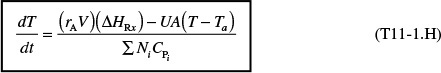
In general most of the PFR and PBR energy balances can be written as
3A. PFR in terms of conversion

3B. PBR in terms of conversion

3C. PBR in terms of molar flow rates

3D. PFR in terms of molar flow rates

4. Batch
5. For Semibatch or unsteady CSTR

6. For multiple reactions in a PFR (q reactions and m species)

End results of manipulating the energy balance (Sections 11.2.4, 12.1, and 12.3)
7. Variable heat exchange fluid temperature, Ta
The equations in Table 11-1 are the ones we will use to solve reaction engineering problems with heat effects.
Nomenclature:

All other symbols are as defined in Chapters 1 through 10.
TABLE 11-1 ENERGY BALANCES OF COMMON REACTORS
Examples of How to Use Table 11-1. We now couple the energy balance equations in Table 11-1 with the appropriate reactor mole balance, rate law, and stoichiometry algorithm to solve reaction engineering problems with heat effects. For example, recall the rate law for a first-order reaction, Equation (E11-1.5) in Example 11-1
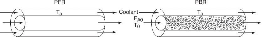
which will be combined with the mole balance to find the concentration, conversion and temperature profiles (i.e., BR, PBR, PFR), exit concentrations, and conversion and temperature in a CSTR. We will now consider four cases of heat exchange in a PFR and PBR: (1) adiabatic, (2) co-current, (3) countercurrent, and (4) constant exchanger temperature. We focus on adiabatic operation in this chapter and the other three cases in Chapter 12.
Case 1: Adiabatic. If the reaction is carried out adiabatically, then we use Equation (T11-1.B) for the reaction A ![]() B in Example 11-1 to obtain
B in Example 11-1 to obtain
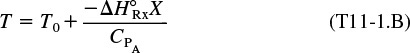
Adiabatic
Consequently, we can now obtain –rA as a function of X alone by first choosing X, then calculating T from Equation (T11-1.B), then calculating k from Equation (E11-1.3), and then finally calculating (–rA) from Equation (E11-1.5).
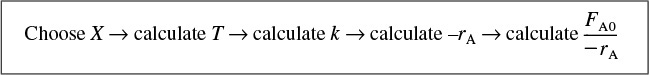
The algorithm
We can use this sequence to prepare a table of (FA0/–rA) as a function of X. We can then proceed to size PFRs and CSTRs. In the absolute worst case scenario, we could use the techniques in Chapter 2 (e.g., Levenspiel plots or the quadrature formulas in Appendix A). However, instead of using a Levenspiel plot, we will most likely use Polymath to solve our coupled differential energy and mole balance equations.

Levenspiel plot
Cases 2, 3, and 4: Correspond to Co-current, Countercurrent, Heat Exchange, and Constant Coolant Temperature TC, respectively (Ch. 12). If there is cooling along the length of a PFR or PBR, we could then apply Equation (T11-1.D) to this reaction to arrive at two coupled differential equations
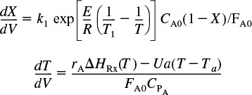
Non-adiabatic PFR
which are easily solved using an ODE solver such as Polymath.
Heat Exchange in a CSTR. Similarly, for the case of the reaction A → B in Example 11-1 carried out in a CSTR, we could use Polymath or MATLAB to solve two nonlinear algebraic equations in X and T. These two equations are the combined mole balance

Non-adiabatic CSTR
and the application of Equation (T11-1.C), which is rearranged in the form
From these three cases, (1) adiabatic PFR and CSTR, (2) PFR and PBR with heat effects, and (3) CSTR with heat effects, one can see how to couple the energy balances and mole balances. In principle, one could simply use Table 11-1 to apply to different reactors and reaction systems without further discussion. However, understanding the derivation of these equations will greatly facilitate the proper application to and evaluation of various reactors and reaction systems. Consequently, we now derive the equations given in Table 11-1.
Why bother? Here is why!!
Why bother to derive the equations in Table 11-1? Because I have found that students can apply these equations much more accurately to solve reaction engineering problems with heat effects if they have gone through the derivation to understand the assumptions and manipulations used in arriving at the equations in Table 11.1. That is, understanding these derivations, students are more likely to put the correct number in the correct equation symbol.
11.3 The User-Friendly Energy Balance Equations
We will now dissect the molar flow rates and enthalpy terms in Equation (11-9) to arrive at a set of equations we can readily apply to a number of reactor situations.
11.3.1 Dissecting the Steady-State Molar Flow Rates to Obtain the Heat of Reaction
To begin our journey, we start with the energy balance equation (11-9) and then proceed to finally arrive at the equations given in Table 11-1 by first dissecting two terms:
1. The molar flow rates, Fi and Fi0
2. The molar enthalpies, Hi, Hi0[Hi ≡ Hi(T), and Hi0 ≡ Hi(T0)]

An animated version of what follows for the derivation of the energy balance can be found in the reaction engineering games “Heat Effects 1” and “Heat Effects 2” on the CRE Web site, www.umich.edu/~elements/5e/index.html. Here, equations move around the screen, making substitutions and approximations to arrive at the equations shown in Table 11-1. Visual learners find these two ICGs a very useful resource.
We will now consider flow systems that are operated at steady state. The steady-state energy balance is obtained by setting (d Êsys/dt) equal to zero in Equation (11-9) in order to yield
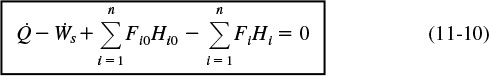
Steady-state energy balance
To carry out the manipulations to write Equation (11-10) in terms of the heat of reaction, we shall use the generic reaction
The inlet and outlet summation terms in Equation (11-10) are expanded, respectively, to
and
where the subscript I represents inert species.
We next express the molar flow rates in terms of conversion. In general, the molar flow rate of species i for the case of no accumulation and a stoichiometric coefficient vi is
Fi = FA0 (Θi + vi X)
Specifically, for Reaction (2-2), ![]() , we have
, we have
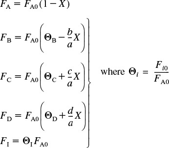
Steady-state operation
We can substitute these symbols for the molar flow rates into Equations (11-11) and (11-12), then subtract Equation (11-12) from (11-11) to give
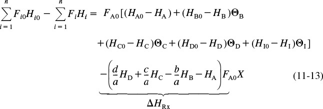
The term in parentheses that is multiplied by FA0 X is called the heat of reaction at temperature T and is designated ΔHRx(T).

Heat of reaction at temperature T
All enthalpies (e.g., HA, HB) are evaluated at the temperature at the outlet of the system volume and, consequently, [ΔHRx (T)] is the heat of reaction at a specific temperature T. The heat of reaction is always given per mole of the species that is the basis of calculation, i.e., species A (joules per mole of A reacted).
Substituting Equation (11-14) into (11-13) and reverting to summation notation for the species, Equation (11-13) becomes

Combining Equations (11-10) and (11-15), we can now write the steady-state, i.e., (![]() ), energy balance in a more usable form:
), energy balance in a more usable form:

Use this form of the steady-state energy balance if the enthalpies are available.
If a phase change takes place during the course of a reaction, this is the form of the energy balance, i.e., Equation (11-16), that must be used.
11.3.2 Dissecting the Enthalpies
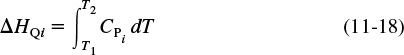
We are neglecting any enthalpy changes resulting from mixing so that the partial molal enthalpies are equal to the molal enthalpies of the pure components. The molal enthalpy of species i at a particular temperature and pressure, Hi, is usually expressed in terms of an enthalpy of formation of species i at some reference temperature TR, ![]() , plus the change in enthalpy, ΔHQi, that results when the temperature is raised from the reference temperature, TR, to some temperature T
, plus the change in enthalpy, ΔHQi, that results when the temperature is raised from the reference temperature, TR, to some temperature T
The reference temperature at which ![]() is given is usually 25°C. For any substance i that is being heated from T1 to T2 in the absence of phase change
is given is usually 25°C. For any substance i that is being heated from T1 to T2 in the absence of phase change
No phase change
Typical units of the heat capacity, CPi, are
A large number of chemical reactions carried out in industry do not involve phase change. Consequently, we shall further refine our energy balance to apply to single-phase chemical reactions. Under these conditions, the enthalpy of species i at temperature T is related to the enthalpy of formation at the reference temperature TR by

If phase changes do take place in going from the temperature for which the enthalpy of formation is given and the reaction temperature T, Equation (11-17) must be used instead of Equation (11-19).
The heat capacity at temperature T is frequently expressed as a quadratic function of temperature; that is
However, while the text will consider only constant heat capacities, the PRS R11.1 on the CRE Web site has examples with variable heat capacities.

To calculate the change in enthalpy (Hi – Hi0) when the reacting fluid is heated without phase change from its entrance temperature, Ti0, to a temperature T, we integrate Equation (11-19) for constant CPi to write

Substituting for Hi and Hi0 in Equation (11-16) yields

Result of dissecting the enthalpies
11.3.3 Relating ΔHRx (T),  , and ΔCP
Recall that the heat of reaction at temperature T was given in terms of the enthalpy of each reacting species at temperature T in Equation (11-14); that is
where the enthalpy of each species is given by

If we now substitute for the enthalpy of each species, we have
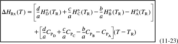
For the generic reaction ![]()
The first term in brackets on the right-hand side of Equation (11-23) is the heat of reaction at the reference temperature TR

The enthalpies of formation of many compounds, ![]() , are usually tabulated at 25°C and can readily be found in the Handbook of Chemistry and Physics and similar handbooks.1 That is, we can look up the heats of formation at TR, then calculate the heat of reaction at this reference temperature. The heat of combustion (also available in these handbooks) can also be used to determine the enthalpy of formation,
, are usually tabulated at 25°C and can readily be found in the Handbook of Chemistry and Physics and similar handbooks.1 That is, we can look up the heats of formation at TR, then calculate the heat of reaction at this reference temperature. The heat of combustion (also available in these handbooks) can also be used to determine the enthalpy of formation, ![]() , and the method of calculation is also described in these handbooks. From these values of the standard heat of formation,
, and the method of calculation is also described in these handbooks. From these values of the standard heat of formation, ![]() , we can calculate the heat of reaction at the reference temperature TR using Equation (11-24).
, we can calculate the heat of reaction at the reference temperature TR using Equation (11-24).
1 CRC Handbook of Chemistry and Physics, 95th ed. (Boca Raton, FL: CRC Press, 2014).
The second term in brackets on the right-hand side of Equation (11-23) is the overall change in the heat capacity per mole of A reacted, ΔCP,
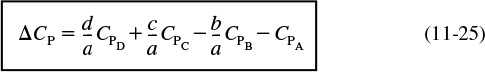
Combining Equations (11-25), (11-24), and (11-23) gives us

Heat of reaction at temperature T
Equation (11-26) gives the heat of reaction at any temperature T in terms of the heat of reaction at a reference temperature (usually 298 K) and the ΔCP term. Techniques for determining the heat of reaction at pressures above atmospheric can be found in Chen.2 For the reaction of hydrogen and nitrogen at 400°C, it was shown that the heat of reaction increased by only 6% as the pressure was raised from 1 atm to 200 atm!
2 N. H. Chen, Process Reactor Design (Needham Heights, MA: Allyn and Bacon, 1983), p. 26.
Calculate the heat of reaction for the synthesis of ammonia from hydrogen and nitrogen at 150°C in kcal/mol of N2 reacted and also in kJ/mol of H2 reacted.
Solution
N2 + 3H2 ![]() 2NH3
2NH3
Calculate the heat of reaction at the reference temperature using the heats of formation of the reacting species obtained from Perry’s Chemical Engineers’ Handbook or the Handbook of Chemistry and Physics.3
3 D. W. Green, and R. H. Perry, eds., Perry’s Chemical Engineers’ Handbook, 8th ed. (New York: McGraw-Hill, 2008).
The enthalpies of formation at 25°C are
Note: The heats of formation of all elements (e.g., H2, N2) are zero at 25°C.
To calculate ![]() , we use Equation (11-24) and we take the heats of formation of the products (e.g., NH3) multiplied by their appropriate stoichiometric coefficients (2 for NH3) minus the heats of formation of the reactants (e.g., N2, H2) multiplied by their stoichiometric coefficient (e.g., 3 for H2, 1 for N2)
, we use Equation (11-24) and we take the heats of formation of the products (e.g., NH3) multiplied by their appropriate stoichiometric coefficients (2 for NH3) minus the heats of formation of the reactants (e.g., N2, H2) multiplied by their stoichiometric coefficient (e.g., 3 for H2, 1 for N2)

or in terms of kJ/mol
Exothermic reaction
The minus sign indicates that the reaction is exothermic. If the heat capacities are constant or if the mean heat capacities over the range 25°C to 150°C are readily available, the determination of ΔHRx at 150°C is quite simple.


in terms of kJ/mol
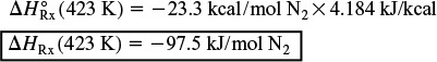
(Recall: 1 kcal = 4.184 kJ)
The heat of reaction based on the moles of H2 reacted is

Analysis: This example showed (1) how to calculate the heat of reaction with respect to a given species, given the heats of formation of the reactants and the products, and (2) how to find the heat of reaction with respect to one species, given the heat of reaction with respect to another species in the reaction. We also saw how the heat of reaction changed as we increased the temperature.
Now that we see that we can calculate the heat of reaction at any temperature, let’s substitute Equation (11-22) in terms of ΔHR(TR) and ΔCP, i.e., Equation (11-26). The steady-state energy balance is now

Energy balance in terms of mean or constant heat capacities
From here on, for the sake of brevity we will let

unless otherwise specified.
In most systems, the work term, ![]() , can be neglected (note the exception in the California Professional Engineers’ Exam Problem P12-6B at the end of Chapter 12). Neglecting
, can be neglected (note the exception in the California Professional Engineers’ Exam Problem P12-6B at the end of Chapter 12). Neglecting ![]() , the energy balance becomes
, the energy balance becomes
In almost all of the systems we will study, the reactants will be entering the system at the same temperature; therefore, Ti0 = T0.
We can use Equation (11-28) to relate temperature and conversion and then proceed to evaluate the algorithm described in Example 11-1. However, unless the reaction is carried out adiabatically, Equation (11-28) is still difficult to evaluate because in nonadiabatic reactors, the heat added to or removed from the system varies along the length of the reactor. This problem does not occur in adiabatic reactors, which are frequently found in industry. Therefore, the adiabatic tubular reactor will be analyzed first.
11.4 Adiabatic Operation
Reactions in industry are frequently carried out adiabatically with heating or cooling provided either upstream or downstream. Consequently, analyzing and sizing adiabatic reactors is an important task.
11.4.1 Adiabatic Energy Balance
In the previous section, we derived Equation (11-28), which relates conversion to temperature and the heat added to the reactor, ![]() . Let’s stop a minute (actually it will probably be more like a couple of days) and consider a system with the special set of conditions of no work,
. Let’s stop a minute (actually it will probably be more like a couple of days) and consider a system with the special set of conditions of no work, ![]() = 0, adiabatic operation
= 0, adiabatic operation ![]() = 0, letting Ti0 = T0 and then rearranging Equation (11-28) into the form
= 0, letting Ti0 = T0 and then rearranging Equation (11-28) into the form
For adiabatic operation, Example 11.1 can now be solved!
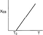
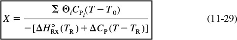
In many instances, the ΔCP (T – TR) term in the denominator of Equation (11-29) is negligible with respect to the ![]() term, so that a plot of X vs. T will usually be linear, as shown in Figure 11-2. To remind us that the conversion in this plot was obtained from the energy balance rather than the mole balance, it is given the subscript EB (i.e., XEB) in Figure 11-2.
term, so that a plot of X vs. T will usually be linear, as shown in Figure 11-2. To remind us that the conversion in this plot was obtained from the energy balance rather than the mole balance, it is given the subscript EB (i.e., XEB) in Figure 11-2.

Relationship between X and T for adiabatic exothermic reactions
Equation (11-29) applies to a CSTR, PFR, or PBR, and also to a BR (as will be shown in Chapter 13). For ![]() = 0 and
= 0 and ![]() = 0, Equation (11-29) gives us the explicit relationship between X and T needed to be used in conjunction with the mole balance to solve a large variety of chemical reaction engineering problems as discussed in Section 11.1.
= 0, Equation (11-29) gives us the explicit relationship between X and T needed to be used in conjunction with the mole balance to solve a large variety of chemical reaction engineering problems as discussed in Section 11.1.
11.4.2 Adiabatic Tubular Reactor
We can rearrange Equation (11-29) to solve for temperature as a function of conversion; that is
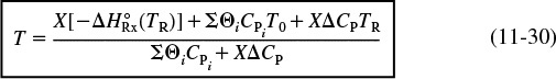
Energy balance for adiabatic operation of PFR
This equation will be coupled with the differential mole balance
to obtain the temperature, conversion, and concentration profiles along the length of the reactor. The algorithm for solving PBRs and PFRs operated adiabatically using a first-order reversible reaction ![]() as an example is shown in Table 11-2.
as an example is shown in Table 11-2.
Table 11-3 gives two different methods for solving the equations in Table 11-2 in order to find the conversion, X, and temperature, T, profiles down the reactor. The numerical technique (e.g., hand calculation) is presented primarily to give insight and understanding to the solution procedure and this understanding is important. With this procedure, one could either construct a Levenspiel plot or use a quadrature formula to find the reactor volume.
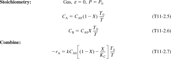
The elementary reversible gas-phase reaction
is carried out in a PFR in which pressure drop is neglected and pure A enters the reactor.
with
and for ΔCP = 0
Energy Balance:
To relate temperature and conversion, we apply the energy balance to an adiabatic PFR. If all species enter at the same temperature, Ti0 = T0.
Solving Equation (11-29) with ![]() = 0,
= 0, ![]() = 0, to obtain T as a function of conversion yields
= 0, to obtain T as a function of conversion yields

If pure A enters and iff ΔCP = 0, then
Equations (T11-2.1) through (T11-2.9) can easily be solved using either Simpson’s rule or an ODE solver.
TABLE 11-2 ADIABATIC PFR/PBR ALGORITHM
Only if my computer is missing.
It is doubtful that anyone would actually use either of these methods unless they had absolutely no access to a computer and they would never get access (e.g., stranded on a desert island with a dead laptop or no satellite connection). The solution to reaction engineering problems today is to use software packages with ordinary differential equation (ODE) solvers, such as Polymath, MATLAB, or Excel, to solve the coupled mole balance and energy balance differential equations.
The numerical technique is presented to provide insight about how the variables (k, Kc, etc.) change as we move down the reactor from V = 0 and X = 0 to Vf and Xf.
Integrating the PFR mole balance,
Choose X → Calculate T → Calculate k → Calculate –rA → Calculate ![]()
1. Set X = 0 .
2. Calculate T using Equation (T11-2.9).
3. Calculate k using Equation (T11-2.3).
4. Calculate KC using Equation (T11-2.4).
5. Calculate T0/T (gas phase).
6. Calculate –rA using Equation (T11-2.7).
7. Calculate (FA0/–rA).
8. If X is less than the exit conversion X3 specified, increment X (i.e., Xi+1 = Xi + ΔX) and go to Step 2.
9. Prepare table of X vs. (FA0/–rA).
10. Use numerical integration formulas given in Appendix A; for example,

with ![]()
Use evaluation techniques discussed in Chapter 2.
B. Ordinary Differential Equation (ODE) Solver

Almost always we will use an ODE solver.


5. Enter parameter values k1, E, R, KC2, ![]() , CP, ΔCP = 0, CA0, T0, T1, T2 .
, CP, ΔCP = 0, CA0, T0, T1, T2 .
6. Enter intial values X = 0, V = 0, and final value reactor volume, V = Vf .
TABLE 11-3 SOLUTION PROCEDURES FOR ELEMENTARY ADIABATIC GAS-PHASE PFR/PBR REACTOR
We will now apply the algorithm in Table 11-2 and solution procedure B in Table 11-3 to a real reaction.
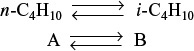
Example 11–3 Adiabatic Liquid-Phase Isomerization of Normal Butane
Normal butane, C4H10, is to be isomerized to isobutane in a plug-flow reactor. Isobutane is a valuable product that is used in the manufacture of gasoline additives. For example, isobutane can be further reacted to form iso-octane. The 2014 selling price of n-butane was $1.5/gal, while the trading price of isobutane was $1.75/gal.†
† Once again, you can buy a cheaper generic brand of n–C4H10 at the Sunday markets in downtown Riça, Jofostan, where there will be a special appearance and lecture by Jofostan’s own Prof. Dr. Sven Köttlov on February 29th, at the CRE booth.

This elementary reversible reaction is to be carried out adiabatically in the liquid phase under high pressure using essentially trace amounts of a liquid catalyst that gives a specific reaction rate of 31.1 h–1 at 360 K. The feed enters at 330 K.
(a) Calculate the PFR volume necessary to process 100,000 gal/day (163 kmol/h) at 70% conversion of a mixture 90 mol % n-butane and 10 mol % i-pentane, which is considered an inert.
(b) Plot and analyze X, Xe, T, and –rA down the length of the reactor.
(c) Calculate the CSTR volume for 40% conversion.
Additional information:

The economic incentive $ = 1.75/gal versus 1.50/gal
Solution
(a) PFR algorithm
The algorithm

with
3. Stoichiometry (liquid phase, υ = υ0):
4. Combine:
5. Energy Balance: Recalling Equation (11-27), we have
From the problem statement
Adiabatic: ![]() = 0
= 0
No work: ![]() = 0
= 0
ΔCP = CPB – CPA = 141 – 141 = 0
Applying the preceding conditions to Equation (11-27) and rearranging gives
Nomenclature Note

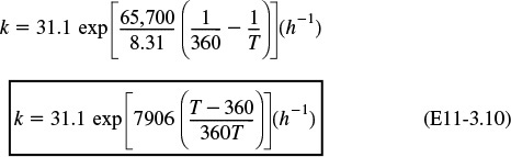
6. Parameter Evaluation:

where T is in degrees Kelvin.
Substituting for the activation energy, T1, and k1 in Equation (E11-3.3), we obtain
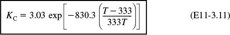
Substituting for ![]() , T2, and KC (T2) in Equation (E11-3.4) yields
, T2, and KC (T2) in Equation (E11-3.4) yields
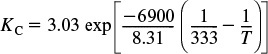
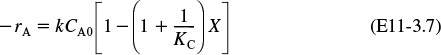
Recalling the rate law gives us
7. Equilibrium Conversion:
At equilibrium
–rA ≡ 0
and therefore we can solve Equation (E11-3.7) for the equilibrium conversion
Because we know KC (T), we can find Xe as a function of temperature.
It’s risky business to ask for 70% conversion in a reversible reaction.
PFR Solution
(a) Find the PFR volume necessary to achieve 70% conversion. This problem statement is risky. Why? Because the adiabatic equilibrium conversion may be less than 70%! Fortunately, it’s not for the conditions here, 0.7 < Xe. In general, we should ask for the reactor volume to obtain 95% of the equilibrium conversion, Xf = 0.95 Xe.
(b) Plot and analyze X, Xe, –rA, and T down the length (volume) of the reactor.
We will solve the preceding set of equations to find the PFR reactor volume using both hand calculations and an ODE computer solution. We carry out the hand calculation to help give an intuitive understanding of how the parameters Xe and –rA vary with conversion and temperature. The computer solution allows us to readily plot the reaction variables along the length of the reactor and also to study the reaction and reactor by varying the system parameters such as CA0 and T0.
Part (a) Solution by hand calculation to perhaps give greater insight and to build on techniques in Chapter 2.
We will now integrate Equation (E11-3.8) using Simpson’s rule after forming a table (E11-3.1) to calculate (FA0/–rA) as a function of X. This procedure is similar to that described in Chapter 2. We now carry out a sample calculation to show how Table E11-3.1 was constructed.
We are only going to do this once!!
For example, for X = 0.2, follow the downward arrows for the sequence of the calculations.
Sample calculation for Table E11-3.1

Continuing in this manner for other conversions, we can complete Table E11-3.1.
I know these are tedious calculations, but someone’s gotta know how to do it.


Use the data in Table E11-3.1 to make a Levenspiel plot, as in Chapter 2.

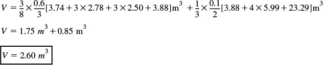
The reactor volume for 70% conversion will be evaluated using the quadrature formulas. Because (FA0/–rA) increases rapidly as we approach the adiabatic equilibrium conversion, 0.71, we will break the integral into two parts
Using Equations (A-24) and (A-22) in Appendix A, we obtain
Why are we doing this hand calculation? If it isn’t helpful, send me an email and you won’t see this again.
Later, 10/10/15: Actually, since this margin note first appeared in 2011, I have had 2 people say to keep the hand calculation in the text so I kept it in.
You probably will never ever carry out a hand calculation similar to the one shown above. So why did we do it? Hopefully, we have given you a more intuitive feel for the magnitude of each of the terms and how they change as one moves down the reactor (i.e., what the computer solution is doing), as well as a demonstration of how the Levenspiel Plots of (FA0/–rA) vs. X in Chapter 2 were constructed. At the exit, V = 2.6 m3, X = 0.7, Xe = 0.715, and T = 360 K.
Part B is the Polymath solution method we will use to solve most all CRE problems with “heat” effects.
Part (b) PFR computer solution and variable profiles
We could have also solved this problem using Polymath or some other ODE solver. The Polymath program using Equations (E11-3.1), (E11-3.7), (E11-3.9), (E11-3.10), (E11-3.11), and (E11-3.12) is shown in Table E11-3.2.

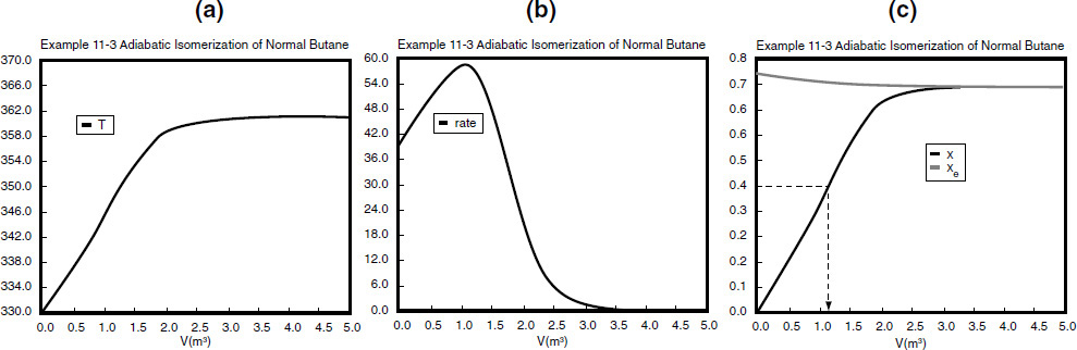
Analysis: The graphical output is shown in Figure E11-3.1. We see from Figure E11-3.1(c) that 1.15 m3 is required for 40% conversion. The temperature and reaction-rate profiles are also shown. Notice anything strange? One observes that the rate of reaction
Look at the shape of the curves in Figure E11-3.1. Why do they look the way they do?
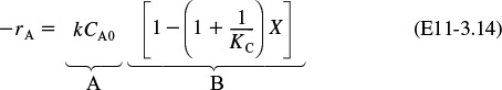
goes through a maximum. Near the entrance to the reactor, T increases as does k, causing term A to increase more rapidly than term B decreases, and thus the rate increases. Near the end of the reactor, term B is decreasing more rapidly than term A is increasing as we approach equilibrium. Consequently, because of these two competing effects, we have a maximum in the rate of reaction. Toward the end of the reactor, the temperature reaches a plateau as the reaction approaches equilibrium (i.e., X ≡ Xe at V ≅ 3.5 m3). As you know, and as do all chemical engineering students at Jofostan University in Riça, at equilibrium (–rA ≅ 0) no further changes in X, Xe, or T take place.
AspenTech: Example 11-3 has also been formulated in AspenTech and can be loaded on your computer directly from the CRE Web site.

Part (c) CSTR Solution
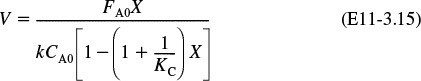
Let’s now calculate the adiabatic CSTR volume necessary to achieve 40% conversion. Do you think the CSTR will be larger or smaller than the PFR to achieve 40% conversion? The mole balance is
Using Equation (E11-3.7) in the mole balance, we obtain
Is VPFR > VCSTR or is VPFR < VCSTR?
From the energy balance, we have Equation (E11-3.9):
![]()
Using Equations (E11-3.10) and (E11-3.11) or from Table E11-3.1, at 347.3 K, we find k and KC to be
Then
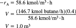
We see that the CSTR volume (1 m3) to achieve 40% conversion in this adiabatic reaction is less than the PFR volume (1.15 m3).
By recalling the Levenspiel plots from Chapter 2, we can see that the reactor volume for 40% conversion is smaller for a CSTR than for a PFR. Plotting (FA0/–rA) as a function of X from the data in Table E11-3.1 is shown here.
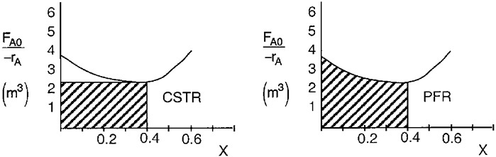
In this example, the adiabatic CSTR volume is less than the PFR volume.
The PFR area (volume) is greater than the CSTR area (volume).
Analysis: In this example we applied the CRE algorithm to a reversible-first-order reaction carried out adiabatically in a PFR and in a CSTR. We note that at the CSTR volume necessary to achieve 40% conversion is smaller than the volume to achieve the same conversion in a PFR. In Figure E11-3.1(c) we also see that at a PFR volume of about 3.5 m3, equilibrium is essentially reached about halfway through the reactor, and no further changes in temperature, reaction rate, equilibrium conversion, or conversion take place farther down the reactor.
11.5 Adiabatic Equilibrium Conversion
The highest conversion that can be achieved in reversible reactions is the equilibrium conversion. For endothermic reactions, the equilibrium conversion increases with increasing temperature up to a maximum of 1.0. For exothermic reactions, the equilibrium conversion decreases with increasing temperature.
For reversible reactions, the equilibrium conversion, Xe, is usually calculated first.
11.5.1 Equilibrium Conversion
Exothermic Reactions. Figure 11-3(a) shows the variation of the concentration equilibrium constant, KC, as a function of temperature for an exothermic reaction (see Appendix C), and Figure 11-3(b) shows the corresponding equilibrium conversion Xe as a function of temperature. In Example 11-3, we saw that for a first-order reaction, the equilibrium conversion could be calculated using Equation (E11-3.13)
First-order reversible reaction
Consequently, Xe can be calculated as a function of temperature directly using either Equations (E11-3.12) and (E11-3.4) or from Figure 11-3(a) and Equation (E11-3.12).
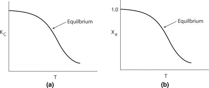
Figure 11-3 Variation of equilibrium constant and conversion with temperature for an exothermic reaction.
For exothermic reactions, the equilibrium conversion decreases with increasing temperature.
We note that the shape of the Xe versus T curve in Figure 11-3(b) will be similar for reactions that are other than first order.
To determine the maximum conversion that can be achieved in an exothermic reaction carried out adiabatically, we find the intersection of the equilibrium conversion as a function of temperature (Figure 11-3(b)) with temperature–conversion relationships from the energy balance (Figure 11-2 and Equation (T11-1.A)), as shown in Figure 11-4.

Adiabatic equilibrium conversion for exothermic reactions
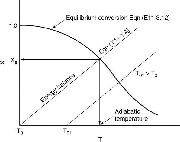
Figure 11-4 Graphical solution of equilibrium and energy balance equations to obtain the adiabatic temperature and the adiabatic equilibrium conversion Xe.
This intersection of the XEB line with the Xe curve gives the adiabatic equilibrium conversion and temperature for an entering temperature T0.
If the entering temperature is increased from T0 to T01, the energy balance line will be shifted to the right and be parallel to the original line, as shown by the dashed line. Note that as the inlet temperature increases, the adiabatic equilibrium conversion decreases.
Example 11–4 Calculating the Adiabatic Equilibrium Temperature
For the elementary liquid-phase reaction
make a plot of equilibrium conversion as a function of temperature.
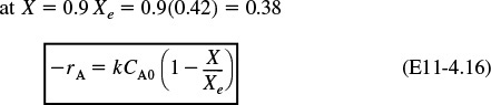
(a) Combine the rate law and stoichiometric table to write –rA as a function of k, CA0, X, and Xe.
(b) Determine the adiabatic equilibrium temperature and conversion when pure A is fed to the reactor at a temperature of 300 K.
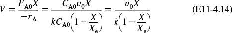
(c) What is the CSTR volume to achieve 90% of the adiabatic equilibrium conversion for υ0 = 5 dm3/min?
Additional information:†
† Jofostan Journal of Thermodynamic Data, Vol. 23, p. 74 (1999).

1. Rate Law:
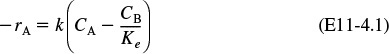
2. Equilibrium: –rA = 0; so
3. Stoichiometry: (υ = υ0) yields
Substituting for Kc in terms of Xe in Equation (E11-4.5) and simplifying

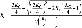
Solving Equation (E11-4.6) for Xe gives

4. Equilibrium Constant: Calculate ΔCP, then Ke (T)
ΔCP = CPB – CPA = 50 – 50 = 0 cal/mol·K
For ΔCP = 0, the equilibrium constant varies with temperature according to the relation

Substituting Equation (E11-4.4) into (E11-4.2), we can calculate the equilibrium conversion as a function of temperature:
5. Equilibrium Conversion from Thermodynamics:
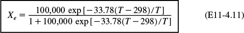
Conversion calculated from equilibrium relationship
The calculations are shown in Table E11-4.1.

6. Energy Balance:
For a reaction carried out adiabatically, the energy balance, Equation (T11-1.A), reduces to
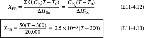
Conversion calculated from energy balance
Data from Table E11-4.1 and the following data are plotted in Figure E11-4.1.
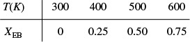
Adiabatic equilibrium conversion and temperature

Figure E11-4.1 Finding the adiabatic equilibrium temperature (Te) and conversion (Xe). Note: Curve uses approximate interpolated points.
For a feed temperature of 300 K, the adiabatic equilibrium temperature is 465 K and the corresponding adiabatic equilibrium conversion is only 0.42.
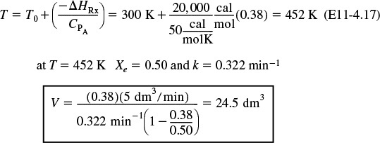
Calculate the CSTR Volume to achieve 90% of the adiabatic equilibrium conversion corresponding to an entering temperature of 300 K.
From the adiabatic energy balance, the temperature corresponding to X = 0.38 is
Analysis: The purpose of this example is to introduce the concept of the adiabatic equilibrium conversion and temperature. The adiabatic equilibrium conversion, Xe, is one of the first things to determine when carrying out an analysis involving reversible reactions. It is the maximum conversion one can achieve for a given entering temperature, T0, and feed composition. If Xe is too low to be economical, try lowering the feed temperature and/or adding inerts. From Equation (E11-4.6), we observe that changing the flow rate has no effect on the equilibrium conversion. For exothermic reactions, the adiabatic conversion decreases with increasing entering temperature T0, and for endothermic reactions the conversion increases with increasing entering T0. One can easily generate Figure E11-4.1 using Polymath with Equations (E11-4.5) and (E11-4.7).
If adding inerts or lowering the entering temperature is not feasible, then one should consider reactor staging.
11.6 Reactor Staging
11.6.1 Reactor Staging with Interstage Cooling or Heating
Conversions higher than those shown in Figure E11-4.1 can be achieved for adiabatic operations by connecting reactors in series with interstage cooling.

In Figure 11-5, we show the case of an exothermic adiabatic reaction taking place in a PBR reactor train. The exit temperature to Reactor 1 is very high, 800 K, and the equilibrium conversion, Xe, is low as is the reactor conversion X1, which approaches Xe. Next, we pass the exit stream from adiabatic reactor 1 through a heat exchanger to bring the temperature back down to 500 K where Xe is high but X is still low. To increase the conversion, the stream then enters adiabatic reactor 2 where the conversion increases to X2, which is followed by a heat exchanger and the process is repeated.
11.6.2 Exothermic Reactions
The conversion–temperature plot for this scheme is shown in Figure 11-6. We see that with three interstage coolers, 88% conversion can be achieved, compared to an equilibrium conversion of 35% for no interstage cooling.
Interstage cooling used for exothermic reversible reactions

Note: Lines and curves are approximate.
Figure 11-6 Increasing conversion by interstage cooling for an exothermic reaction.
11.6.3 Endothermic Reactions
Another example of the need for interstage heat transfer in a series of reactors can be found when upgrading the octane number of gasoline. The more compact the hydrocarbon molecule for a given number of carbon atoms, the higher the octane rating (see Section 10.3.5). Consequently, it is desirable to convert straight-chain hydrocarbons to branched isomers, naphthenes, and aromatics. The reaction sequence is

Typical values for gasoline composition
Gasoline

The first reaction step (k1) is slow compared to the second step, and each step is highly endothermic. The allowable temperature range for which this reaction can be carried out is quite narrow: Above 530°C undesirable side reactions occur, and below 430°C the reaction virtually does not take place. A typical feed stock might consist of 75% straight chains, 15% naphthas, and 10% aromatics.
One arrangement currently used to carry out these reactions is shown in Figure 11-7. Note that the reactors are not all the same size. Typical sizes are on the order of 10-m to 20-m high and 2 m to 5 m in diameter. A typical feed rate of gasoline is approximately 200 m3/h at 2 atm. Hydrogen is usually separated from the product stream and recycled.

Summer 2015 $2.89/gal for octane number (ON) ON = 89
Because the reaction is endothermic, the equilibrium conversion increases with increasing temperature. A typical equilibrium curve and temperature conversion trajectory for the reactor sequence are shown in Figure 11-8.
Interstage heating
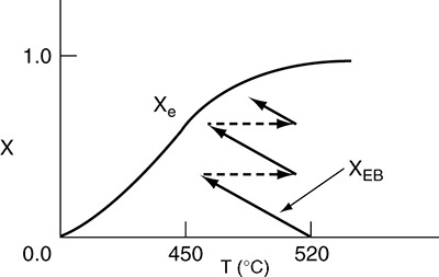
Figure 11-8 Temperature–conversion trajectory for interstage heating of an endothermic reaction analogous to Figure 11-6.
Example 11–5 Interstage Cooling for Highly Exothermic Reactions
What conversion could be achieved in Example 11-4 if two interstage coolers that had the capacity to cool the exit stream to 350 K were available? Also, determine the heat duty of each exchanger for a molar feed rate of A of 40 mol/s. Assume that 95% of the equilibrium conversion is achieved in each reactor. The feed temperature to the first reactor is 300 K.
Solution
1. Calculate Exit Temperature
For the reaction in Example 11-4, i.e.,
we saw that for an entering temperature of 300 K the adiabatic equilibrium conversion was 0.42. For 95% of the equilibrium conversion (Xe = 0.42), the conversion exiting the first reactor is 0.4. The exit temperature is found from a rearrangement of Equation (E11-4.7)
We now cool the gas stream exiting the reactor at 460 K down to 350 K in a heat exchanger (Figure E11-5.1).
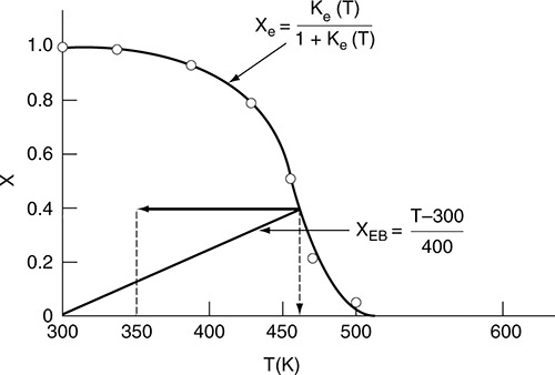
Figure E11-5.1 Determining exit conversion and temperature in the first stage. Note: Curve uses approximate interpolated points.
2. Calculate the Heat Load
There is no work done on the reaction gas mixture in the exchanger, and the reaction does not take place in the exchanger. Under these conditions (Fi|in = Fi|out), the energy balance given by Equation (11-10)
for ![]() = 0 becomes
= 0 becomes
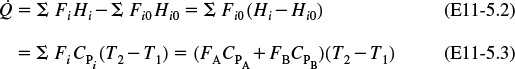
Energy balance on the reaction gas mixture in the heat exchanger
But CPA = CPB
Also, for this example, FA0 = FA + FB

That is, 220 kcal/s must be removed to cool the reacting mixture from 460 K to 350 K for a feed rate of 40 mol/s.
3. Second Reactor
Now let’s return to determine the conversion in the second reactor. Rearranging Equation (E11-4.7) for the second reactor
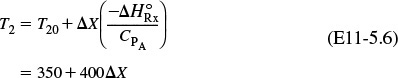
The conditions entering the second reactor are T = 350 K and X = 0.4. The energy balance starting from this point is shown in Figure E11-5.2. The corresponding adiabatic equilibrium conversion is 0.63. Ninety-five percent of the equilibrium conversion is 60% and the corresponding exit temperature is T = 350 + (0.6 – 0.4)400 = 430 K.

Figure E11-5.2 Three reactors in series with interstage cooling. Note: Curve uses approximate interpolated points.
4. Heat Load
The heat-exchange duty to cool the reacting mixture from 430 K back to 350 K can again be calculated from Equation (E11-5.5)

5. Subsequent Reactors
For the third and final reactor, we begin at T0 = 350 K and X = 0.6 and follow the line representing the equation for the energy balance along to the point of intersection with the equilibrium conversion, which is X = 0.8. Consequently, the final conversion achieved with three reactors and two interstage coolers is (0.95) (0.8) = 0.76.
Analysis: For highly exothermic reactions carried out adiabatically, reactor staging with interstage cooling can be used to obtain high conversions. One observes that the exit conversion and temperature from the first reactor are 40% and 450 K respectively, as shown by the energy balance line. The exit stream at this conversion is then cooled to 350 K where it enters the second reactor. In the second reactor, the overall conversion and temperature increase to 60% and 430 K. The slope of X versus T from the energy balance is the same as the first reactor. This example also showed how to calculate the heat load on each exchanger. We also note that the heat load on the third exchanger will be less than the first exchanger because the exit temperature from the second reactor (430 K) is lower than that of the first reactor (450 K). Consequently, less heat needs to be removed by the third exchanger.
11.7 Optimum Feed Temperature
We now consider an adiabatic reactor of fixed size or catalyst weight and investigate what happens as the feed temperature is varied. The reaction is reversible and exothermic. At one extreme, using a very high feed temperature, the specific reaction rate will be large and the reaction will proceed rapidly, but the equilibrium conversion will be close to zero. Consequently, very little product will be formed. At the other extreme of low feed temperatures, little product will be formed because the reaction rate is so low.
We now consider the adiabatic reversible exothermic reaction
Combining the thermodynamic Equations (E11-3.12) and (E11-3.4) for this reaction, we can construct the equilibrium conversion, Xe, as a function of temperature shown in Figure 11-9. Inserting the appropriate value for CPi, Θi, and –ΔHRx into the adiabatic energy balance, Equation (T11-1.A) for this reacting system we obtain

We now plot the adiabatic energy balances, Equation (11-31), for three different entering temperatures T0 in Figure 11-9. Next, we look for the intersections of the conversion calculated from the energy balance, XEB, with the equilibrium conversion Xe calculated from thermodynamics. We see that for an entering temperature of T0 = 600 K the adiabatic equilibrium conversion Xe is 0.15, and the corresponding adiabatic equilibrium temperature is 620 K. However, for an entering temperature of T0 = 350 K, Xe is 0.75 and the corresponding adiabatic equilibrium temperature is 450 K.
We next plot the corresponding conversion profiles down the length of the reactor for entering temperatures 350 K, 500 K and 600 K as shown in Figure 11-10. Because the reactor temperature increases as we move along the reactor, the equilibrium conversion, Xe, also varies and decreases along the length of the reactor, as shown by the dashed line in Figure 11-10. We also see that at the high entering temperature, 600 K, the rate is very rapid and equilibrium is achieved very near the reactor entrance. The corresponding conversion profiles down the length of the reactor for these temperatures are shown in Figure 11-10. The equilibrium conversion, which can be calculated from Equation (E11-4.2) for a first-order reaction also varies along the length of the reactor, as shown by the dashed line in Figure 11-10. We also see that because of the high entering temperature, the rate is very rapid at the inlet and equilibrium is achieved very near the reactor entrance. The solid line is calculated by combining the energy mole balances and solving numerically.
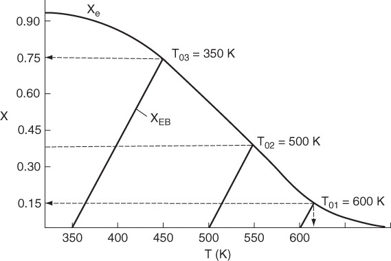
Observe how the conversion profile changes as the entering temperature is decreased from 600 K.
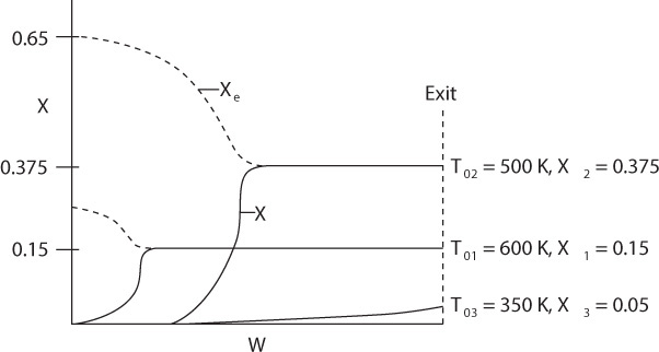
We notice that the conversion and temperature increase very rapidly over a short distance (i.e., a small amount of catalyst). This sharp increase is sometimes referred to as the “point” or temperature at which the reaction “ignites.” If the inlet temperature were lowered to 500 K, the corresponding equilibrium conversion would increase to 0.375; however, the reaction rate is slower at this lower temperature so that this conversion is not achieved until closer to the end of the reactor. If the entering temperature were lowered further to 350 K, the corresponding equilibrium conversion would be 0.75, but the rate is so slow that a conversion of 0.05 is achieved for the specified catalyst weight in the reactor. At a very low feed temperature, the specific reaction rate will be so small that virtually all of the reactant will pass through the reactor without reacting. It is apparent that with conversions close to zero for both high and low feed temperatures, there must be an optimum feed temperature that maximizes conversion. As the feed temperature is increased from a very low value, the specific reaction rate will increase, as will the conversion. The conversion will continue to increase with increasing feed temperature until the equilibrium conversion is approached in the reaction. Further increases in feed temperature for this exothermic reaction will only decrease the conversion due to the decreasing equilibrium conversion. This optimum inlet temperature is shown in Figure 11-11.
Optimum inlet temperature

Closure. Virtually all reactions that are carried out in industry involve heat effects. This chapter provides the basis to design reactors that operate at steady state and that involve heat effects. To model these reactors, we simply add another step to our algorithm; this step is the energy balance. One of the goals of this chapter is to understand each term of the energy balance and how it was derived. We have found that if the reader understands the various steps in the derivation, he/she will be in a much better position to apply the equation correctly. In order not to overwhelm the reader while studying reactions with heat effects, we have broken up the different cases and only consider the case of reactors operated adiabatically in this chapter. Chapter 12 will focus on reactors with heat exchange. Chapter 13 will focus on reactors not operated at steady state. An industrial adiabatic reaction concerning the manufacture of sulfuric acid provides a number of practical details is included on the CRE Web site in PRS R12.4.
Summary
For the reaction
1. The heat of reaction at temperature T, per mole of A, is
2. The mean heat capacity difference, ΔCP, per mole of A is
where CPi is the mean heat capacity of species i between temperatures TR and T.
3. When there are no phase changes, the heat of reaction at temperature T is related to the heat of reaction at the standard reference temperature TR by
4. The steady-state energy balance on a system volume V is
We now couple the first four building blocks Mole Balance, Rate Law, Stoichiometry, and Combine with the fifth block, the Energy Balance, to solve nonisothermal reaction engineering problems as shown in the Closure box for this chapter.
5. For adiabatic operation (![]() ≡ 0) of a PFR, PBR, CSTR, or batch reactor (BR), and neglecting
≡ 0) of a PFR, PBR, CSTR, or batch reactor (BR), and neglecting ![]() , we solve Equation (S11-4) for the adiabatic conversion-temperature relationship, which is
, we solve Equation (S11-4) for the adiabatic conversion-temperature relationship, which is

Solving Equation (S11-5) for the adiabatic temperature–conversion relationship:
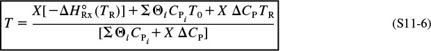
Using Equation (S11-4), one can solve nonisothermal adiabatic reactor problems to predict the exit conversion, concentrations, and temperature.
CRE Web Site Materials
• Expanded Material
1. Puzzle Problem “What’s Wrong with this Solution?”
• Learning Resources
1. Summary Notes
2. PFR/PBR Solution Procedure for a Reversible Gas-Phase Reaction
• Living Example Problems
1. Example 11-3 Polymath Adiabatic Isomerization of Normal Butane
2. Example 11-3 Formulated in AspenTech—Download from the CRE Web site

A step-by-step AspenTech tutorial is given on the CRE Web site.
• Professional Reference Shelf
R11.1. Variable Heat Capacities. Next, we want to arrive at a form of the energy balance for the case where heat capacities are strong functions of temperature over a wide temperature range. Under these conditions, the mean values of the heat capacity may not be adequate for the relationship between conversion and temperature. Combining the heat of reaction with the quadratic form of the heat capacity
CPi = αi + βiT + γiT2
we find that the heat capacity as a function of temperature is

Example 11-4 is reworked for the case of variable heat capacities.
Questions and Problems
The subscript to each of the problem numbers indicates the level of difficulty: A, least difficult; D, most difficult.

In each of the questions and problems, rather than just drawing a box around your answer, write a sentence or two describing how you solved the problem, the assumptions you made, the reasonableness of your answer, what you learned, and any other facts that you want to include. See the Preface for additional generic parts (x), (y), (z) to the home problems.

Before solving the problems, state or sketch qualitatively the expected results or trends.
Questions
Q11-1A Read over the problems at the end of this chapter. Make up an original problem that uses the concepts presented in this chapter. To obtain a solution:
(a) Make up your data and reaction.
(b) Use a real reaction and real data. See Problem P5-1A for guidelines.
(c) Prepare a list of safety considerations for designing and operating chemical reactors. What would be the first four items on your list? (See www.sache.org and www.siri.org/graphics.) The August 1985 issue of Chemical Engineering Progress may be useful.
(d) Recalling selectivity in Chapter 8, why and how would you use reactor staging to improve selectivity of series, parallel, and complex reactions?
(e) Which example on the CRE Web site Lecture Notes for Chapter 11 was the most difficult?
(f) What if you were asked to give an everyday example that demonstrates the principles discussed in this chapter? (Would sipping a teaspoon of Tabasco or other hot sauce be one?)
(g) Rework Problem P2-9D (page 67) for the case of adiabatic operation.
(a) Example 11-1. How would this example change if a CSTR were used instead of a PFR?
(b) Example 11-2. (1) What would the heat of reaction be if 50% inerts (e.g., helium) were added to the system? (2) What would be the % error if the ΔCP term were neglected?

(c) Example 11-3. (1) What if the butane reaction were carried out in a 0.8-m3 PFR that can be pressurized to very high pressures? (2) What inlet temperature would you recommend? Is there anoptimum inlet temperature? (3) Plot the heat that must be removed along the reactor (![]() vs. V) to maintain isothermal operation.
vs. V) to maintain isothermal operation.
(d) AspenTech Example 11-3. Download the AspenTech program from the CRE Web site. (1) Repeat P11-2B (c) using AspenTech. (2) Vary the inlet flow rate and temperature, and describe what you find.
(e) Example 11-4. (1) Make a plot of the equilibrium conversion as a function of entering temperature, T0. (2) What do you observe at high and low T0? (3) Make a plot of Xe versus T0 when the feed is equal molar in inerts that have the same heat capacity. (4) Compare the plots of Xe versus T0 with and without inerts and describe what you find.
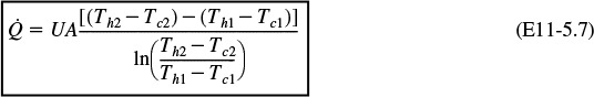
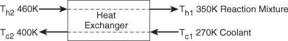
(f) Example 11-5. (1) Determine the molar flow rate of cooling water (CPw = 18 cal/mol·K) necessary to remove 220 kcal/s from the first exchanger. The cooling water enters at 270 K and leaves at 400 K. (2) Determine the necessary heat exchanger area A (m2) for an overall heat-transfer coefficient, U, of 100 cal/s·m2·K. You must use the log-mean driving force in calculating A.
P11-2A For elementary reaction
the equilibrium conversion is 0.8 at 127°C and 0.5 at 227°C. What is the heat of reaction?
P11-3B The equilibrium conversion is shown below as a function of catalyst weight

Please indicate which of the following statements are true and which are false. Explain each case.
(a) The reaction could be first-order endothermic and carried out adiabatically.
(b) The reaction is first-order endothermic and the reactor is heated along its length with Ta being constant.
(c) The reaction is second-order exothermic and cooled along the length of the reactor with Ta being constant.
(d) The reaction is second-order exothermic and carried out adiabatically.
P11-4A The elementary, irreversible, organic liquid-phase reaction
A + B → C
is carried out adiabatically in a flow reactor. An equal molar feed in A and B enters at 27°C, and the volumetric flow rate is 2 dm3/s and CA0 = 0.1 kmol/m3.
Additional information:
PFR
(a) Plot and then analyze the conversion and temperature as a function of PFR volume up to where X = 0.85. Describe the trends.
(b) What is the maximum inlet temperature one could have so that the boiling point of the liquid (550 K) would not be exceeded even for complete conversion?
(c) Plot the heat that must be removed along the reactor (![]() vs. V) to maintain isothermal operation.
vs. V) to maintain isothermal operation.
(d) Plot and then analyze the conversion and temperature profiles up to a PFR reactor volume of 10 dm3 for the case when the reaction is reversible with KC = 10 m3/kmol at 450 K. Plot the equilibrium conversion profile. How are the trends different than part (a)? (Ans.: When V = 10 dm3 then X = 0.0051, Xeq = 0517)
CSTR
(e) What is the CSTR volume necessary to achieve 90% conversion?
BR
(f) The reaction is next carried out in a 25 dm3 batch reactor charged with NA0 = 10 moles. Plot the number of moles of A, NA, the conversion, and the temperature as a function of time.
P11-5A The elementary, irreversible gas-phase reaction
A → B + C
is carried out adiabatically in a PFR packed with a catalyst. Pure A enters the reactor at a volumetric flow rate of 20 dm3/s, at a pressure of 10 atm, and a temperature of 450 K.
Additional information:

All heats of formation are referenced to 273 K.
(a) Plot and then analyze the conversion and temperature down the plug-flow reactor until an 80% conversion (if possible) is reached. (The maximum catalyst weight that can be packed into the PFR is 50 kg.) Assume that ΔP = 0.0.
(b) Vary the inlet temperature and describe what you find.
(c) Plot the heat that must be removed along the reactor (![]() vs. V) to maintain isothermal operation.
vs. V) to maintain isothermal operation.
(d) Now take the pressure drop into account in the PBR with ρb = 1 kg/dm3.
The reactor can be packed with one of two particle sizes. Choose one.
α = 0.019/kg-cat for particle diameter D1
α = 0.0075/kg-cat for particle diameter D2
(e) Plot and then analyze the temperature, conversion, and pressure along the length of the reactor. Vary the parameters and P0 to learn the ranges of values in which they dramatically affect the conversion.
(f) Apply one or more of the six ideas in Preface Table P-4, page xxviii, to this problem.
P11-6B The irreversible endothermic vapor-phase reaction follows an elementary rate law
and is carried out adiabatically in a 500-dm3 PFR. Species A is fed to the reactor at a rate of 10 mol/min and a pressure of 2 atm. An inert stream is also fed to the reactor at 2 atm, as shown in Figure P11-6B. The entrance temperature of both streams is 1100 K.

Additional information:
(a) First derive an expression for CA01 as a function of CA0 and ΘI .
(b) Sketch the conversion and temperature profiles for the case when no inerts are present. Using a dashed line, sketch the profiles when a moderate amount of inerts are added. Using a dotted line, sketch the profiles when a large amount of inerts are added. Qualitative sketches are fine. Describe the similarities and differences between the curves.
(c) Sketch or plot and then analyze the exit conversion as a function of ΘI. Is there a ratio of the entering molar flow rates of inerts (I) to A (i.e., ΘI = FI0/FA0) at which the conversion is at a maximum? Explain why there “is” or “is not” a maximum.
(d) What would change in parts (b) and (c) if reactions were exothermic and reversible with ![]() and KC = 2 dm3/mol at 1100 K?
and KC = 2 dm3/mol at 1100 K?
(e) Sketch or plot FB for parts (c) and (d), and describe what you find.
(f) Plot the heat that must be removed along the reactor (![]() vs. V) to maintain isothermal operation for pure A fed and an exothermic reaction. Part (f) is “C” level of difficulty, i.e., P11-6C(f).
vs. V) to maintain isothermal operation for pure A fed and an exothermic reaction. Part (f) is “C” level of difficulty, i.e., P11-6C(f).
P11-7B The gas-phase reversible reaction
is carried out under high pressure in a packed-bed reactor with pressure drop. The feed consists of both inerts I and Species A with the ratio of inerts to the species A being 2 to 1. The entering molar flow rate of A is 5 mol/min at a temperature of 300 K and a concentration of 2 mol/dm3. Work this problem in terms of volume. Hint: V = W/ρB, ![]() .
.
Additional information:
(a) Adiabatic Operation. Plot X, Xe, p, T, and the rate of disappearance as a function of V up to V = 40 dm3. Explain why the curves look the way they do.
(b) Vary the ratio of inerts to A (0 ≤ ΘI ≤ 10) and the entering temperature, and describe what you find.
(c) Plot the heat that must be removed along the reactor (![]() vs. V) to maintain isothermal operation. Part (c) is “C” level of difficulty.
vs. V) to maintain isothermal operation. Part (c) is “C” level of difficulty.
We will continue this problem in Chapter 12.
P11-8B Algorithm for reaction in a PBR with heat effects
The elementary gas-phase reaction
is carried out in a packed-bed reactor. The entering molar flow rates are FA0 = 5 mol/s, FB 0 = 2FA0, and F1 = 2FA 0 with CA0 = 0.2 mol/dm3. The entering temperature is 325 K and a coolant fluid is available at 300 K.
Additional information:
(a) Write the mole balance, the rate law, KC as a function of T, k as a function of T, and CA, CB, CC as a function of X, p, and T.
(b) Write the rate law as a function of X, p, and T.
(c) Show the equilibrium conversion is
and then plot Xe vs. T.
(d) What are ∑ΘiCPi, ΔCP, T0, entering temperature T1 (rate law), and T2 (equilibrium constant)?
(e) Write the energy balance for adiabatic operation.
(f) Case 1 Adiabatic Operation. Plot and then analyze Xe, X, p, and T versus W when the reaction is carried out adiabatically. Describe why the profiles look the way they do. Identify those terms that will be affected by inerts. Sketch what you think the profiles Xe, X, p, and T will look like before you run the Polymath program to plot the profiles. (Ans.: At W = 800 kg then X ≌ Xeq = 0.3583)
(g) Plot the heat that must be removed along the reactor (![]() vs. V) to maintain isothermal operation. Part (g) is “C” level of difficulty, i.e., P11-9C(g).
vs. V) to maintain isothermal operation. Part (g) is “C” level of difficulty, i.e., P11-9C(g).
is carried out adiabatically in a series of staged packed-bed reactors with interstage cooling (see Figure 11-5). The lowest temperature to which the reactant stream may be cooled is 27°C. The feed is equal molar in A and B, and the catalyst weight in each reactor is sufficient to achieve 99.9% of the equilibrium conversion. The feed enters at 27°C and the reaction is carried out adiabatically. If four reactors and three coolers are available, what conversion may be achieved?
Additional information:

First prepare a plot of equilibrium conversion as a function of temperature. (Partial ans.: T = 360 K, Xe = 0.984; T = 520 K, Xe = 0.09; T = 540 K, Xe = 0.057)
P11-10A Figure P11-10A shows the temperature–conversion trajectory for a train of reactors with interstage heating. Now consider replacing the interstage heating with injection of the feed stream in three equal portions, as shown in Figure P11-10A:
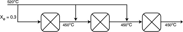
Sketch the temperature-conversion trajectories for (a) an endothermic reaction with entering temperatures as shown, and (b) an exothermic reaction with the temperatures to and from the first reactor reversed, i.e., T0 = 450°C.
Supplementary Reading
1. An excellent development of the energy balance is presented in
ARIS, R., Elementary Chemical Reactor Analysis. Upper Saddle River, NJ: Prentice Hall, 1969, Chaps. 3 and 6.
A number of example problems dealing with nonisothermal reactors may or may not be found in
BURGESS, THORNTON W., The Adventures of Old Man Coyote. New York: Dover Publications, Inc., 1916.
BUTT, JOHN B., Reaction Kinetics and Reactor Design, Revised and Expanded, 2nd ed. New York: Marcel Dekker, Inc., 1999.
WALAS, S.M., Chemical Reaction Engineering Handbook of Solved Problems. Amsterdam: Gordon and Breach, 1995. See the following solved problems: 4.10.1, 4.10.08, 4.10.09, 4.10.13, 4.11.02, 4.11.09, 4.11.03, 4.10.11.
For a thorough discussion on the heat of reaction and equilibrium constant, one might also consult
DENBIGH, K. G., Principles of Chemical Equilibrium, 4th ed. Cambridge: Cambridge University Press, 1981.
2. The heats of formation, Hi (T), Gibbs free energies, Gi (TR), and the heat capacities of various compounds can be found in
GREEN, D. W. and R. H. PERRY, eds., Chemical Engineers’ Handbook, 8th ed. New York: McGraw-Hill, 2008.
REID, R. C., J. M. PRAUSNITZ, and T. K. SHERWOOD, The Properties of Gases and Liquids, 3rd ed. New York: McGraw-Hill, 1977.
WEAST, R. C., ed., CRC Handbook of Chemistry and Physics, 94th ed. Boca Raton, FL: CRC Press, 2013.