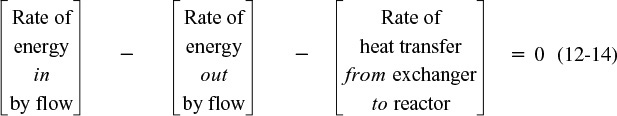
12. Steady-State Nonisothermal Reactor Design—Flow Reactors with Heat Exchange
Research is to see what everybody else sees, and to think what nobody else has thought.
—Albert Szent-Gyorgyi
12.1 Steady-State Tubular Reactor with Heat Exchange
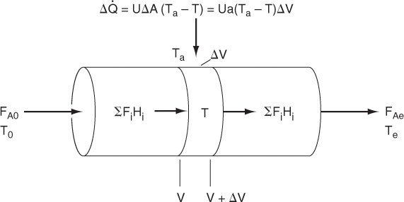
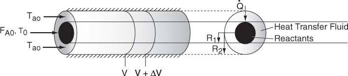
In this section, we consider a tubular reactor in which heat is either added or removed through the cylindrical walls of the reactor (Figure 12-1). In modeling the reactor, we shall assume that there are no radial gradients in the reactor and that the heat flux through the wall per unit volume of reactor is as shown in Figure 12-1.1
1 Radial gradients are discussed in Chapters 17 and 18.
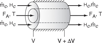
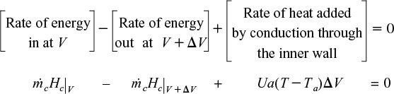
12.1.1 Deriving the Energy Balance for a PFR
We will carry out an energy balance on the volume ΔV. There is no work done, i.e., ![]() , so Equation (11-10) becomes
, so Equation (11-10) becomes
The heat flow to the reactor, ![]() , is given in terms of the overall heat-transfer coefficient, U, the heat exchange area, ΔA, and the difference between the ambient temperature, Ta, and the reactor temperature T
, is given in terms of the overall heat-transfer coefficient, U, the heat exchange area, ΔA, and the difference between the ambient temperature, Ta, and the reactor temperature T
where a is the heat exchange area per unit volume of reactor. For a tubular reactor
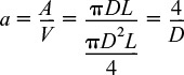
where D is the reactor diameter. Substituting for ![]() in Equation (12-1), dividing by ΔV, and then taking the limit as ΔV → 0, we get
in Equation (12-1), dividing by ΔV, and then taking the limit as ΔV → 0, we get
Expanding
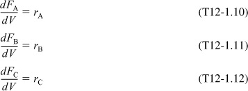
From a mole balance on species i, we have
Differentiating the enthalpy Equation (11-19) with respect to V
Substituting Equations (12-3) and (12-4) into Equation (12-2), we obtain
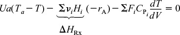
Rearranging, we arrive at
This form of the energy balance will also be applied to multiple reactions.
and
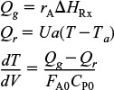
where
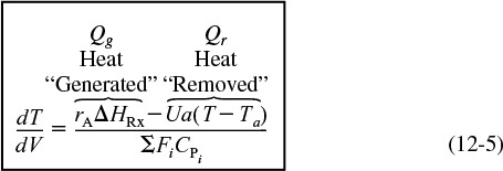
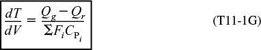
Qg = rA ΔHRx
Qr = Ua(T − Ta)
which is Equation (T11-1G) in Table 11-1 on pages 498–500.
For exothermic reactions, Qg will be a positive number. We note that when the heat “generated,” Qg, is greater than the heat “removed,” Qr (i.e., Qg > Qr), the temperature will increase down the reactor. When Qr > Qg, the temperature will decrease down the reactor.
For endothermic reactions, Qg will be a negative number and Qr will also be a negative number because Ta > T. The temperature will decrease if (–Qg) > (–Qr) and increase if (–Qr) > (–Qg).
Equation (12-5) is coupled with the mole balances on each species, Equation (12-3). Next, we express rA as a function of either the concentrations for liquid systems or molar flow rates for gas systems, as described in Chapter 4. We will use the molar flow rate form of the energy balance for membrane reactors and also extend this form to multiple reactions.
We could also write Equation (12-5) in terms of conversion by recalling Fi = FA0(Θi + viX) and substituting this expression into the denominator of Equation (12-5).
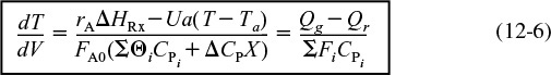
PFR energy balance
For a packed-bed reactor dW = ρb dV where ρb is the bulk density
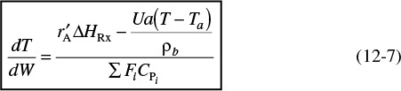
PBR energy balance
Equations (12-6) and (12-7) are also given in Table 11-1 as Equations (T11-1D) and (T11-1F). As noted earlier, having gone through the derivation to these equations, it will be easier to apply them accurately to CRE problems with heat effects.
12.1.2 Applying the Algorithm to Flow Reactors with Heat Exchange
We continue to use the algorithm described in the previous chapters and simply add a fifth building block, the energy balance.
Gas Phase
If the reaction is in gas phase and pressure drop is included, there are four differential equations that must be solved simultaneously. The differential equation describing the change in temperature with volume (i.e., distance) as we move down the reactor
Energy balance
must be coupled with the mole balance
Mole balance
and with the pressure drop equation
Pressure drop
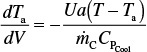
and solved simultaneously. If the temperature of the heat-exchange fluid, Ta, varies down the reactor, we must add the energy balance on the heat-exchange fluid. In the next section, we will derive the following equation for co-current heat transfer
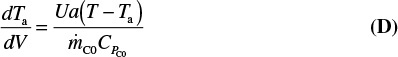
Heat exchanger
along with the equation for countercurrent heat transfer. A variety of numerical schemes can be used (e.g., Polymath) to solve these coupled differential equations: (A), (B), (C), and (D).
Numerical integration of the coupled differential equations (A) to (D) is required.
Liquid Phase
For liquid-phase reactions, the rate is not a function of total pressure, so our mole balance is
Consequently, we need to only solve equations (A), (D), and (E) simultaneously.
12.2 Balance on the Heat-Transfer Fluid
12.2.1 Co-current Flow
The heat-transfer fluid will be a coolant for exothermic reactions and a heating medium for endothermic reactions. If the flow rate of the heat-transfer fluid is sufficiently high with respect to the heat released (or absorbed) by the reacting mixture, then the heat-transfer fluid temperature will be virtually constant along the reactor. In the material that follows, we develop the basic equations for a coolant to remove heat from exothermic reactions; however, these same equations apply to endothermic reactions where a heating medium is used to supply heat.
We now carry out an energy balance on the coolant in the annulus between R1 and R2, and between V and V + ΔV, as shown in Figure 12-2. The mass flow rate of the heat-exchange fluid (e.g., coolant) is ![]() . We will consider the case when the reactor is cooled and the outer radius of the coolant channel R2 is insulated. Recall that by convention
. We will consider the case when the reactor is cooled and the outer radius of the coolant channel R2 is insulated. Recall that by convention ![]() is the heat added to the system.
is the heat added to the system.
For co-current flow, the reactant and the coolant flow in the same direction.
The energy balance on the coolant in the volume between V and (V + ΔV) is
where Ta is the temperature of the heat transfer fluid, i.e., coolant, and T is the temperature of the reacting mixture in the inner tube.
Dividing by ΔV and taking limit as ΔV → 0
Analogous to Equation (12-4), the change in enthalpy of the coolant can be written as
The variation of coolant temperature Ta down the length of reactor is
The equation is valid whether the heat-transfer fluid is a coolant or a heating medium.
Typical heat-transfer fluid temperature profiles are shown here for both exothermic and endothermic reactions when the heat transfer fluid enters at Ta0.
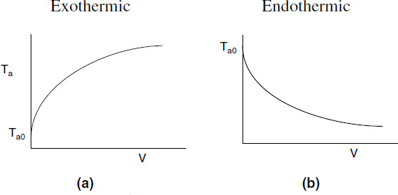
Figure 12-3 Heat-transfer fluid temperature profiles for co-current heat exchanger. (a) Coolant. (b) Heating medium.
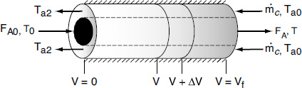
12.2.2 Countercurrent Flow
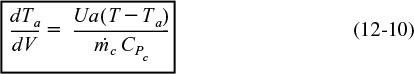
In countercurrent heat exchange, the reacting mixture and the heat-transfer fluid (e.g., coolant) flow in opposite directions. At the reactor entrance, V = 0, the reactants enter at temperature T0, and the coolant exits at temperature Ta2. At the end of the reactor, the reactants and products exit at temperature T, while the coolant enters at Ta0.
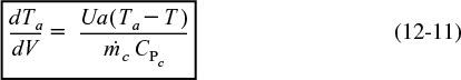
Again, we write an energy balance over a differential reactor volume to arrive at
At the entrance, V = 0 ∴ X = 0 and Ta = Ta2.
At the exit, V = Vf ∴ Ta = Ta0.
We note that the only difference between Equations (12-10) and (12-11) is a minus sign, i.e., (T – Ta) vs. (Ta – T).
The solution to a countercurrent flow problem to find the exit conversion and temperature requires a trial-and-error procedure.
1. Consider an exothermic reaction where the coolant stream enters at the end of the reactor (V = Vf) at a temperature Ta0, say 300 K. We have to carry out a trial-and-error procedure to find the temperature of the coolant exiting the reactor.
2. Guess an exit coolant temperature Ta2 at the feed entrance (X = 0, V = 0) to the reactor to be Ta2 = 340 K, as shown in Figure 12-5(a).
3. Use an ODE solver to calculate X, T, and Ta as a function of V.
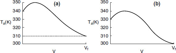
Trial and error procedure required
We see from Figure 12-5(a) that our guess of 340 K for Ta2 at the feed entrance (V = 0 and X = 0) gives an entering temperature of the coolant of 310 K (V = Vf), which does not match the actual entering coolant temperature of 300 K.
4. Now guess another coolant temperature at V = 0 and X = 0 of, say, 330 K. After carrying out the simulation with this guess, we see from Figure 12-5(b) that a coolant temperature at V = 0 of Ta2 = 330 K will give a coolant entering temperature at Vf of 300 K, which matches the actual Ta0.
TABLE 12-1 PROCEDURE TO SOLVE FOR THE EXIT CONDITIONS FOR PFRs WITH COUNTERCURRENT HEAT EXCHANGE
12.3 Algorithm for PFR/PBR Design with Heat Effects
We now have all the tools to solve reaction engineering problems involving heat effects in PFRs and PBRs for the cases of both constant and variable coolant temperatures.
Table 12-2 gives the algorithm for the design of PFRs and PBRs with heat exchange: In Case A Conversion is the reaction variable and in Case B Molar Flow Rates are the reaction variables. The procedure in Case B must be used to analyze multiple reactions with heat effects.
A. Conversion as the reaction variable
1. Mole Balance:

2. Rate Law:
for ΔCP ≅ 0.
3. Stoichiometry (gas phase, no ΔP):
4. Energy Balances:
B. Molar flow rates as the reaction variable
1. Mole Balances:

2. Rate Law: Elementary reaction
3. Stoichiometry (gas phase, no ΔP):
4. Energy Balance:
Heat Exchangers:
If the heat-transfer fluid (e.g., coolant) temperature, Ta, is not constant, the energy balance on the heat-exchange fluid gives
Variable coolant temperature

Co-current flow
Countercurrent flow
where ![]() is the mass flow rate of the coolant (e.g., kg/s, and CPc is the heat capacity of the coolant (e.g., kJ/kg·K).
is the mass flow rate of the coolant (e.g., kg/s, and CPc is the heat capacity of the coolant (e.g., kJ/kg·K).
5. Parameter Evaluation:
Now we enter all the explicit equations with the appropriate parameter values.
Case A: Conversion as the Independent Variable
k1, E, R, CT0, Ta, T0, T1, T2, KC2, ΘB, ![]() , CPA, CPB, CPC, Ua
, CPA, CPB, CPC, Ua
with initial values T0 and X = 0 at V = 0 and final values: Vf = ______
Case B: Molar Flow Rates as the Independent Variables
Same as Case A, except that the inlet values FA0, and FB0 are specified instead of X at V = 0.
Note: In Problem P12-3B, the equations in this table have been applied directly to a PBR (recall that we simply use W = ρbV). Problem P12-3B is also a Living Example Problem (12-T12-3) on the CRE Web site, www.umich.edu/~elements/5e/index.html. Download this Living Example Problem from the CRE Web site and vary the cooling rate, flow rate, entering temperature, and other parameters to get an intuitive feel of what happens in flow reactors with heat effects. After carrying out this exercise, go to the ![]() that is at the very end of Chapter 12 Summary Notes on the CRE Web site and answer the questions in the workbook and also at the end of entitled PBR with Heat Exchange and Variable Coolant Flow Rate.
that is at the very end of Chapter 12 Summary Notes on the CRE Web site and answer the questions in the workbook and also at the end of entitled PBR with Heat Exchange and Variable Coolant Flow Rate.
The following figures in Table 12-2 show representative profiles that would result from solving the above equations. The reader is encouraged to download the Living Example Problem for Table 12-2 and vary a number of parameters, as discussed in P12-3B. Be sure you can explain why these curves look the way they do.
Be sure you can explain why these curves look the way they do.

12.3.1 Applying the Algorithm to an Exothermic Reaction
When plant engineer Maxwell Anthony looked up the vapor pressure at the exit to the adiabatic reactor in Example 11-3, where the temperature is 360 K, he learned the vapor pressure was about 1.5 MPa for isobutene, which is greater than the rupture pressure of the glass vessel the company had hoped to use. Fortunately, when Max looked in the storage shed, he found there was a bank of 10 tubular reactors, each of which was 5 m3. The bank reactors were double-pipe heat exchangers with the reactants flowing in the inner pipe and with Ua = 5,000 kJ/m3·h·K. Max also bought some thermodynamic data from one of the companies he found on the Internet that did Colorimeter experiments to find ΔHRx for various reactions. One of the companies had the value of ΔHRx for his reaction on sale this week for the low, low price of $25,000.00. For this value of ΔHRx the company said it is best to use an initial concentration of A of 1.86 mol/dm3. The entering temperature of the reactants is 305 K and the entering coolant temperature is 315 K. The mass flow rate of the coolant, ![]() , is 500 kg/h and the heat capacity of the coolant, CPC, is 28 kJ/kg·K. The temperature in any one of the reactors cannot rise above 325 K. Carry out the following analyses with the newly purchased values from the Internet:
, is 500 kg/h and the heat capacity of the coolant, CPC, is 28 kJ/kg·K. The temperature in any one of the reactors cannot rise above 325 K. Carry out the following analyses with the newly purchased values from the Internet:
(a) Co-current heat exchange: Plot X, Xe, T, Ta, and –rA, down the length of the reactor.
(b) Countercurrent heat exchange: Plot X, Xe, T, Ta, and –rA down the length of the reactor.
(c) Constant ambient temperature, Ta: Plot X, Xe, T, and –rA down the length of the reactor.
(d) Adiabatic operation: Plot X, Xe, T, Ta, and –rA, down the length of the reactor.
(e) Compare parts (a) through (d) above and write a paragraph describing what you find.
Additional information
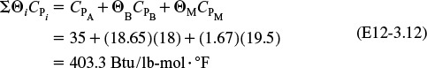
Recall from Example 11-3 that CPA = 141 kJ/kmol · K, CP0 = ΣΘiCPi = 159 kJ/kmol • K, and data from the company Maxwell got off the Internet are ΔHRx = –34,500 kJ/kmol with ΔCPA = 0 and CA0 = 1.86 kmol/m3
Solution
We shall first solve part (a), the co-current heat exchange case and then make small changes in the Polymath program for parts (b) through (d).
For each of the ten reactors in parallel
The mole balance, rate law, and stoichiometry are the same as in the adiabatic case previously discussed in Example 11-3; that is,
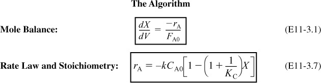
Same as Example 11-3
with
Energy Balance
The energy balance on the reactor is

Part (a) Co-current Heat Exchange
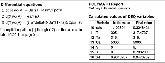
We are now going to solve the coupled, ordinary differential and explicit equations (E11-3.1), (E11-3.7), (E11-3.10), (E11-3.11), (E11-3.12), and (E12-1.1), and the appropriate heat-exchange balance using Polymath. After entering these equations we will enter the parameter values. By using co-current heat exchange as our Polymath base case, we only need to change one line in the program for each of the other three cases and solve for the profiles of X, Xe, T, Ta, and –rA, and not have to re-enter the program.
For co-current flow, the balance on the heat transfer fluid is

with Ta = 310 K at V = 0. The Polymath program and solution are shown in Table E12-1.1.
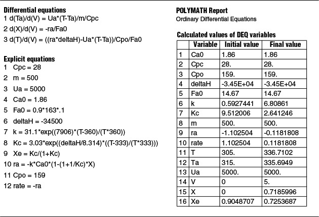
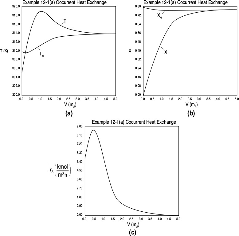
Figure E12-1.1 Profiles down the reactor for co-current heat exchange (a) temperature, (b) conversion, (c) reaction rate.
Analysis: Part (a) Co-current Exchange: We note that reactor temperature goes through a maximum. Near the reactor entrance, the reactant concentrations are high and therefore the reaction rate is high [c.f. Figure E12-1.1(a)] and Qg > Qr. Consequently, the temperature and conversion increase with increasing reactor volume while Xe decreases because of the increasing temperature. Eventually, X and Xe come close together (V = 0.95 m3) and the rate becomes very small as the reaction approaches equilibrium. At this point, the reactant conversion X cannot increase unless Xe increases. We also note that when the ambient heat-exchanger temperature, Ta, and the reactor temperature, T, are essentially equal, there is no longer a temperature driving force to cool the reactor. Consequently, the temperature does not change farther down the reactor, nor does the equilibrium conversion, which is only a function of temperature.
Part (b) Countercurrent Heat Exchange:
For countercurrent flow, we only need to make two changes in the program. First, multiply the right-hand side of Equation (E12-1.2) by minus one to obtain

Next, we guess Ta at V = 0 and see if it matches Ta0 at V = 5 m3. If it doesn’t, we guess again. In this example, we will guess Ta (V = 0) = 340.3 K and see if Ta = Ta0 = 315 K at V = 5 m3.


Good guess!
What a lucky guess we made of 340.3 K at V = 0 to find Ta0 = 315 K!! The variable profiles are shown in Figure E12-1.2.
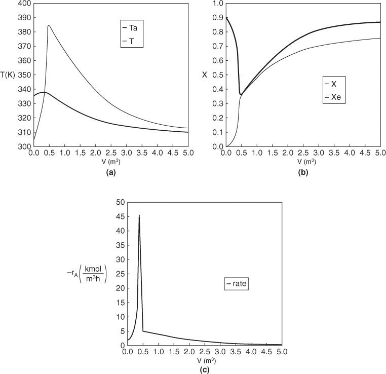
Figure E12-1.2 Profiles down the reactor for counter current heat exchange (a) temperature, (b) conversion, (c) reaction rate.
Analysis: Part (b) Countercurrent Exchange: We note that near the entrance to the reactor, the coolant temperature is above the reactant entrance temperature. However, as we move down the reactor, the reaction generates “heat” and the reactor temperature rises above the coolant temperature. We note that Xe reaches a minimum (corresponding to the reactor temperature maximum) near the entrance to the reactor. At this point (V = 0.5 m3), X cannot increase above Xe. As we move down the reactor, the reactants are cooled and the reactor temperature decreases allowing X and Xe to increase. A higher exit conversion, X, and equilibrium conversion, Xe, are achieved in the countercurrent heat-exchange system than for the co-current system.
Part (c) Constant Ta
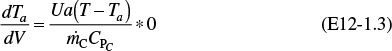
For constant Ta, use the Polymath program in part (a), but multiply the right side of Equation (E12-1.2) by zero in the program, i.e.,
The initial and final values are shown in the Polymath report and the variable profiles are shown in Figure E12-1.3 on page 553.
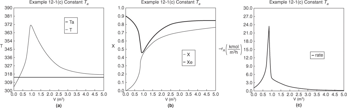
Figure E12-1.3 Profiles down the reactor for constant heat-exchange fluid temperature Ta; (a) temperature, (b) conversion, (c) reaction rate.
Analysis: Part (c) Constant Ta: When the coolant flow rate is sufficiently large, the coolant temperature, Ta, will be essentially constant. If the reactor volume is sufficiently large, the reactor temperature will eventually reach the coolant temperature, as is the case here. At this exit temperature, which is the lowest achieved in this example, the equilibrium conversion, Xe, is the largest of the four cases studied in this example.
Part (d) Adiabatic Operation
In Example 11-3, we solved for the temperature as a function of conversion and then used that relationship to calculate k and KC. An easier way is to solve the general or base case of a heat exchanger for co-current flow and write the corresponding Polymath program. Next, use Polymath [part (a)], but multiply the parameter Ua by zero, i.e.,
Ua = 5,000 * 0
and run the simulation again.

The initial and exit conditions are shown in the Polymath report, while the profiles of T, X, Xe, and –rA are shown in Figure E12-1.4.
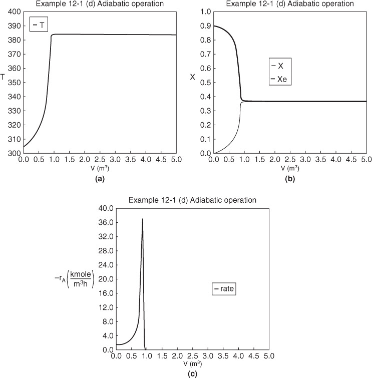
Figure E12-1.4 Profiles down the reactor for adiabatic reactor; (a) temperature, (b) conversion, (c) reaction rate.
Analysis: Part (d) Adiabatic Operation. Because there is no cooling, the temperature of this exothermic reaction will continue to increase down the reactor until equilibrium is reached, X = Xe = 0.365 at T = 384 K, which is the adiabatic equilibrium temperature. The profiles for X and Xe are shown in Figure E12-1.4(b) where one observes that Xe decreases down the reactor because of the increasing temperature until it becomes equal to the reactor conversion (i.e., X ≡ Xe), which occurs circa 0.9 m3. There is no change in temperature, X or Xe, after this point because the reaction rate is virtually zero and thus the remaining reactor volume serves no purpose.
Finally, Figure E12-1.4(c) shows –rA increases as we move down the reactor as the temperature increases, reaching a maximum and then decreasing until X and Xe approach each other and the rate becomes virtually zero.
Overall Analysis: This is an extremely important example, as we applied our CRE PFR algorithm with heat exchange to a reversible exothermic reaction. We analyzed four types of heat-exchanger operations. We see the countercurrent exchanger gives the highest conversion and adiabatic operation gives the lowest conversion.
12.3.2 Applying the Algorithm to an Endothermic Reaction
In Example 12-1 we studied the four different types of heat exchanger on an exothermic reaction. In this section we carry out the same study on an endothermic reaction.
Example 12–2 Production of Acetic Anhydride
Jeffreys, in a treatment of the design of an acetic anhydride manufacturing facility, states that one of the key steps is the endothermic vapor-phase cracking of acetone to ketene and methane is2
2 G. V. Jeffreys, A Problem in Chemical Engineering Design: The Manufacture of Acetic Anhydride, 2nd ed. (London: Institution of Chemical Engineers, 1964).
CH3COCH3 → CH2CO+CH4
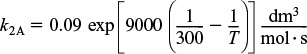
He states further that this reaction is first-order with respect to acetone and that the specific reaction rate can be expressed by
Gas-phase endothermic reaction examples:
1. Adiabatic
2. Heat exchange Ta is constant
3. Co-current heat exchange with variable Ta
4. Counter current exchange with variable Ta
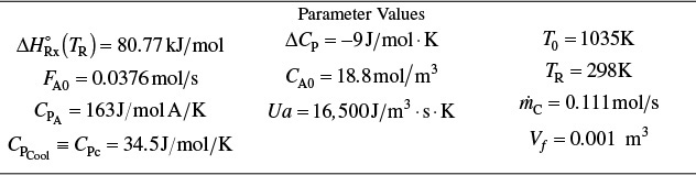
where k is in reciprocal seconds and T is in Kelvin. In this design it is desired to feed 7850 kg of acetone per hour to a tubular reactor. The reactor consists of a bank of 1000 one-inch schedule 40 tubes. We shall consider four cases of heat exchanger operation. The inlet temperature and pressure are the same for all cases at 1035 K and 162 kPa (1.6 atm) and the entering heating-fluid temperature available is 1250 K.
A bank of 1000 one-in. schedule 40 tubes 1.79 m in length corresponds to 1.0 m3 (0.001 m3/tube = 1.0 dm3/tube) and gives 20% conversion. Ketene is unstable and tends to explode, which is a good reason to keep the conversion low. However, the pipe material and schedule size should be checked to learn if they are suitable for these temperatures and pressures. The heat-exchange fluid has a flow rate, ![]() , of 0.111 mol/s, with a heat capacity of 34.5 J/mol·K.
, of 0.111 mol/s, with a heat capacity of 34.5 J/mol·K.
Case 1 The reactor is operated adiabatically.
Case 2 Constant heat-exchange fluid temperature Ta = 1250 K
Case 3 Co-current heat exchange with Ta0 = 1250 K
Case 4 Countercurrent heat exchange with Ta0 = 1250 K
Additional information
Solution
Let A = CH3COCH3, B = CH2CO, and C = CH4. Rewriting the reaction symbolically gives us
A → B + C
Algorithm for a PFR with Heat Effects
Rearranging (E12-2.1)
3. Stoichiometry (gas-phase reaction with no pressure drop):

4. Combining yields
Before combining Equations (E12-2.2) and (E12-2.6), it is first necessary to use the energy balance to determine T as a function of X.
5. Energy Balance:
a. Reactor balance
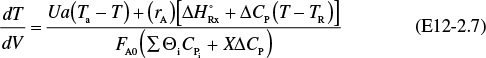
b. Heat Exchanger. We will use the heat-exchange fluid balance for co-current flow as our base case. We will then show how we can very easily modify our ODE solver program (e.g., Polymath) to solve for the other cases by simply multiplying the appropriate line in the code by either zero or minus one.
For co-current flow:
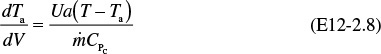
6. Calculation of Mole Balance Parameters on a Per Tube Basis:
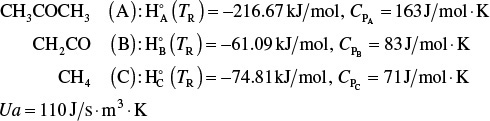
7. Calculation of Energy Balance Parameters:
Thermodynamics:
a. ![]() : At 298 K, using the standard heats of formation
: At 298 K, using the standard heats of formation

b. ΔCP: Using the mean heat capacities
ΔCP = CPB + CPC – CPA = (83 + 71 – 163) J/mol · K
ΔCP = –9 J/mol · K
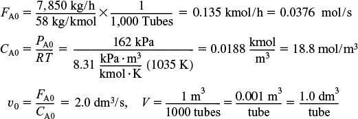
Energy balance. From the adiabatic case in Case I, we already have CP, CPA. The heat-transfer area per unit volume of pipe is
Combining the overall heat-transfer coefficient with the area yields
Ua = 16,500 J/m3 · s · K
Adiabatic endothermic reaction in a PFR
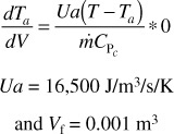
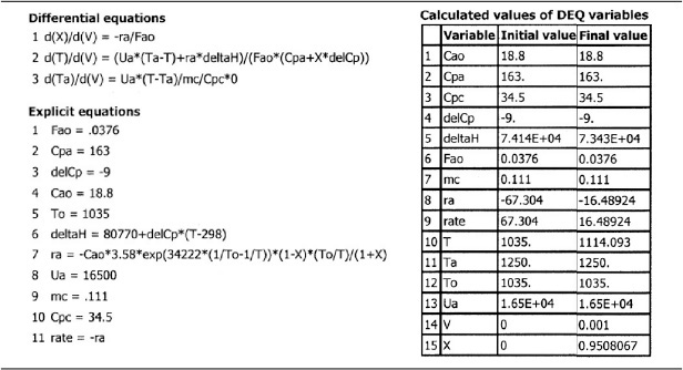
We will solve for all four cases of heat exchanger operation for this endothermic reaction example in the same way we did for the exothermic reaction in Example 12-1. That is, we will write the Polymath equations for the case of co-current heat exchange and use that as the base case. We will then manipulate the different terms in the heat-transfer fluid balance (Equations 12-10 and 12-11) to solve for the other cases, starting with the adiabatic case where we multiply the heat-transfer coefficient in the base case by zero.
Case 1 Adiabatic
We are going to start with the adiabatic case first to show the dramatic effects of how the reaction dies out as the temperature drops. In fact, we are going to extend each to a volume of 5 dm3 to observe this effect and to show the necessity of adding a heat exchanger. For the adiabatic case, we simply multiply the value of Ua in our Polymath program by zero. No other changes are necessary. For the adiabatic case, the answer will be the same whether we use a bank of 1000 reactors, each a 1-dm3 reactor, or one of 1 m3. To illustrate how an endothermic reaction can virtually die out completely, let’s extend the single-pipe volume from 1 dm3 to 5 dm3.
Ua = 16,500 * 0
The Polymath program is shown in Table E12-2.2. Figure E12-2.1 shows the graphical output.
Death of a reaction


Analysis: Case 1 Adiabatic Operation: As temperature drops, so does k and hence the rate, –rA, drops to an insignificant value. Note that for this adiabatic endothermic reaction, the reaction virtually dies out after 3.5 dm3, owing to the large drop in temperature, and very little conversion is achieved beyond this point. One way to increase the conversion would be to add a diluent such as nitrogen, which could supply the sensible heat for this endothermic reaction. However, if too much diluent is added, the concentration, and hence the rate, will be quite low. On the other hand, if too little diluent is added, the temperature will drop and virtually extinguish the reaction. How much diluent to add is left as an exercise. Figures E12-2.1 (a) and (b) give the reactor volume as 5 dm3 in order to show the reaction “dying out.” However, because the reaction is nearly complete near the entrance to the reactor, i.e., –rA ≅ 0, we are going to study and compare the heat-exchange systems in a 1-dm3 reactor (0.001 m3) in the next three cases.
Case 2 Constant heat-exchange fluid temperature, Ta
We make the following changes in our program on line 3 of the base case (a)
The profiles for T, X, and –rA are shown below.
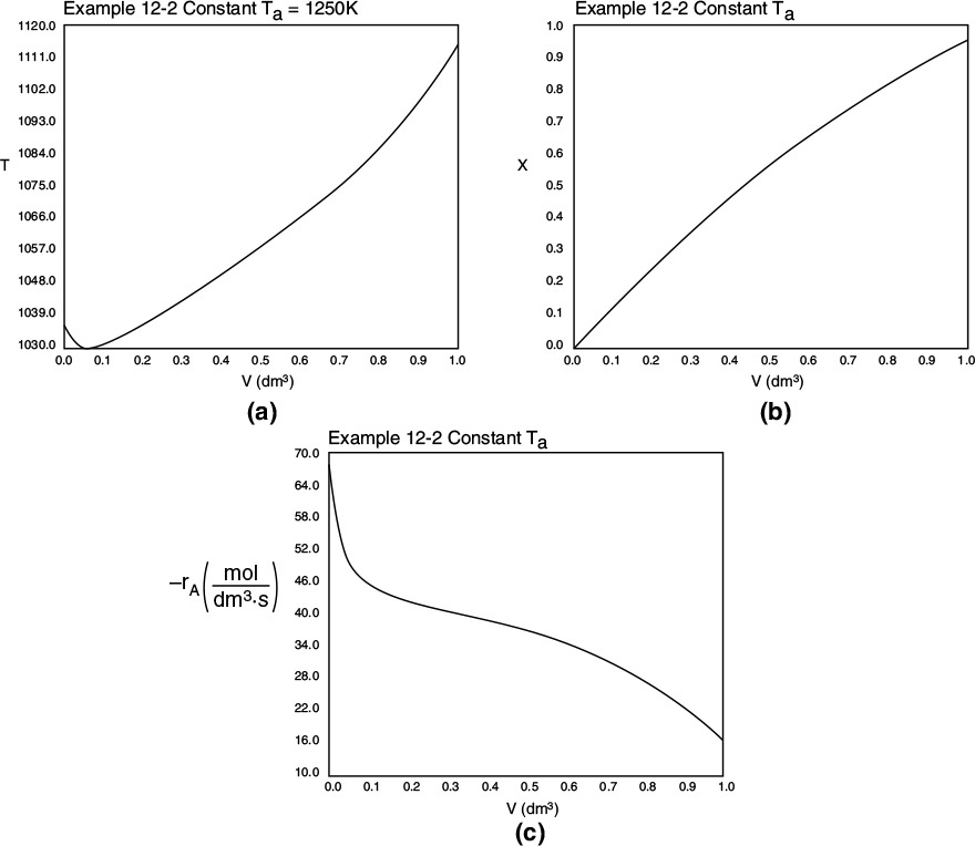
Figure E12-2.2 Profiles for constant heat exchanger fluid temperature, Ta; (a) temperature, (b) conversion, (c) reaction rate.
Analysis: Case 2 Constant Ta: Just after the reactor entrance, the reaction temperature drops as the sensible heat from the reacting fluid supplies the energy for the endothermic reaction. This temperature drop in the reactor also causes the rate of reaction to drop. As we move farther down the reactor, the reaction rate drops further as the reactants are consumed. Beyond V = 0.08 dm3, the heat supplied by the constant Ta heat exchanger becomes greater than that “consumed” by the endothermic reaction and the reactor temperature rises. In the range between V = 0.2 dm3 and V = 0.6 dm3, the rate decreases slowly owing to the depletion of reactants, which is counteracted, to some extent, by the increase in temperature and hence the rate constant k. Consequently, we are eventually able to achieve an exit conversion of 95%.
Case 3 Co-current Heat Exchange
The energy balance on a co-current exchanger is
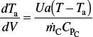
with Ta0 = 1250 K at V = 0

The variable profiles for T, Ta, X, and –rA are shown below. Because the reaction is endothermic, Ta needs to start off at a high temperature at V = 0.
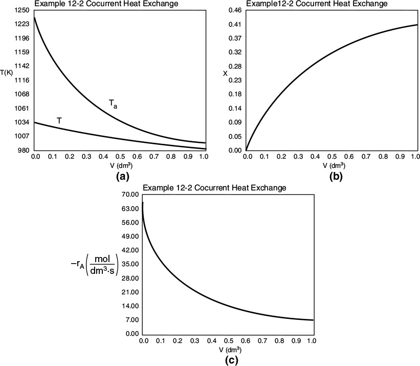
Figure E12-2.3 Profiles down the reactor for an endothermic reaction with co-current heat exchange; (a) temperature, (b) conversion, and (c) reaction rate.
Analysis: Case 3 Co-Current Exchange: In co-current heat exchange, we see that the heat-exchanger fluid temperature, Ta, drops rapidly initially and then continues to drop along the length of the reactor as it supplies the energy to the heat drawn by the endothermic reaction. Eventually Ta decreases to the point where it approaches T and the rate of heat exchange is small; as a result, the temperature of the reactor, T, continues to decrease, as does the rate, resulting in a small conversion. Because the reactor temperature for co-current exchange is lower than that for Case 2 constant Ta, the reaction rate will be lower. As a result, significantly less conversion will be achieved than in the case of constant heat-exchange temperature Ta.
Case 4 Countercurrent Heat Exchange

For countercurrent exchange, we first multiply the rhs of the co-current heat-exchanger energy balance by –1, leaving the rest of the Polymath program in Table 12-2.5 the same.

Next, guess Ta (V = 0) = 995.15 K to obtain Ta0 = 1250 K at V = 0.001m3. (Don’t you believe for a moment 995.15 K was my first guess.) Once this match is obtained as shown in Table E12-2.5, we can report the profiles shown in Figure E12-2.4.

Good guess!
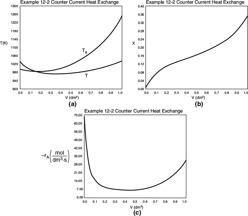
Figure E12-2.4 Profiles down the reactor for countercurrent heat exchange; (a) temperature, (b) conversion, (c) reaction rate.
Analysis: Case 4 Countercurrent Exchange: At the front of the reactor, V = 0, the reaction takes place very rapidly, drawing energy from the sensible heat of the gas and causing the gas temperature to drop because the heat exchanger cannot supply energy at an equal or greater rate to that being drawn by the endothermic reaction. Additional “heat” is lost at the entrance in the case of countercurrent exchange because the temperature of the exchange fluid, Ta, is below the entering reactor temperature, T. One notes there is a minimum in the reaction rate, –rA, profile that is rather flat. In this flat region, the rate is “virtually” constant between V = 0.2 dm3 and V = 0.8 dm3, because the increase in k caused by the increase in T is balanced by the decrease in rate brought about by the consumption of reactants. Just past the middle of the reactor, the rate begins to increase slowly as the reactants become depleted and the heat exchanger now supplies energy at a rate greater than the reaction draws energy and, as a result, the temperature eventually increases. This lower temperature coupled with the consumption of reactants causes the rate of reaction to be low in the plateau, resulting in a lower conversion than either the co-current or constant Ta heat exchange cases.
AspenTech: Example 12-2 has also been formulated in AspenTech and can be downloaded on your computer directly from the CRE Web site.
12.4 CSTR with Heat Effects
In this section we apply the general energy balance [Equation (11-22)] to a CSTR at steady state. We then present example problems showing how the mole and energy balances are combined to design reactors operating adiabatically and non-adiabatically.
In Chapter 11 the steady-state energy balance was derived as
Recall that ![]() is the shaft work, i.e., the work done by the stirrer or mixer in the CSTR on the reacting fluid inside the CSTR. Consequently, because the convention that
is the shaft work, i.e., the work done by the stirrer or mixer in the CSTR on the reacting fluid inside the CSTR. Consequently, because the convention that ![]() done by the system on the surroundings is positive, the CSTR stirrer work will be a negative number, e.g.,
done by the system on the surroundings is positive, the CSTR stirrer work will be a negative number, e.g., ![]() = –1,000 J/s. (See problem P12-6B, a California Professional Engineers’ Exam Problem.)
= –1,000 J/s. (See problem P12-6B, a California Professional Engineers’ Exam Problem.)
These are the forms of the steady-state balance we will use.
Note: In many calculations the CSTR mole balance derived in Chapter 2
(FA0X = –rAV)
will be used to replace the term following the brackets in Equation (11-28), that is, (FA0X) will be replaced by (–rAV) to arrive at Equation (12-12).
Rearranging yields the steady-state energy balance
Although the CSTR is well mixed and the temperature is uniform throughout the reaction vessel, these conditions do not mean that the reaction is carried out isothermally. Isothermal operation occurs when the feed temperature is identical to the temperature of the fluid inside the CSTR.
The  Term in the CSTR
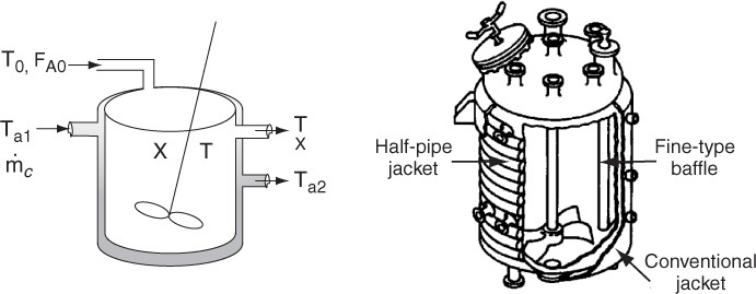
12.4.1 Heat Added to the Reactor,
Figure 12-6 shows the schematics of a CSTR with a heat exchanger. The heat-transfer fluid enters the exchanger at a mass flow rate ![]() (e.g., kg/s) at a temperature Ta1 and leaves at a temperature Ta2. The rate of heat transfer from the exchanger to the reactor fluid at temperature T is3
(e.g., kg/s) at a temperature Ta1 and leaves at a temperature Ta2. The rate of heat transfer from the exchanger to the reactor fluid at temperature T is3
3 Information on the overall heat-transfer coefficient may be found in C. J. Geankoplis, Transport Processes and Unit Operations, 4th ed. (Englewood Cliffs, NJ: Prentice Hall, 2003), p. 300.
For exothermic reactions (T>Ta2>Ta1)
The following derivations, based on a coolant (exothermic reaction), apply also to heating mediums (endothermic reaction). As a first approximation, we assume a quasi-steady state for the coolant flow and neglect the accumulation
For endothermic reactions (T1a>T2a>T)
term (i.e., dTa/dt = 0). An energy balance on the heat-exchanger fluid entering and leaving the exchanger is
Energy balance on heat-exchanger fluid
where CPc is the heat capacity of the heat exchanger fluid and TR is the reference temperature. Simplifying gives us
Solving Equation (12-16) for the exit temperature of the heat-exchanger fluid yields

From Equation (12-16)
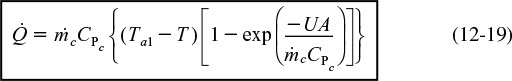
Substituting for Ta2 in Equation (12-18), we obtain
Heat transfer to a CSTR
For large values of the heat-exchanger fluid flow rate, ![]() , the exponent will be small and can be expanded in a Taylor series (e–x = 1 – x + . . .) where second-order terms are neglected in order to give
, the exponent will be small and can be expanded in a Taylor series (e–x = 1 – x + . . .) where second-order terms are neglected in order to give

where Ta1 ≅ Ta2 = Ta.
Valid only for large heat-transfer fluid flow rates!!
With the exception of processes involving highly viscous materials such as Problem P12-6B, a California Professional Engineers’ Exam Problem, the work done by the stirrer can usually be neglected. Setting ![]() in Equation (11-27) to zero, neglecting ΔCP, substituting for
in Equation (11-27) to zero, neglecting ΔCP, substituting for ![]() , and rearranging, we have the following relationship between conversion and temperature in a CSTR
, and rearranging, we have the following relationship between conversion and temperature in a CSTR
Solving for X
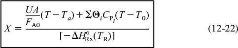
Equation (12-22) is coupled with the mole balance equation
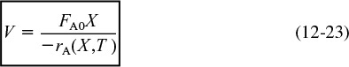
to design CSTRs.
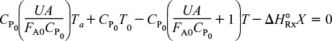
We now will further rearrange Equation (12-21) after letting
then
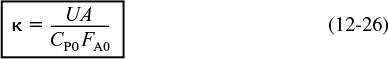
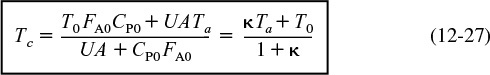
Let κ and TC be non-adiabatic parameters defined by
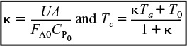
Non-adiabatic CSTR heat exchange parameters: κ and Tc
Then
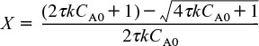
The parameters κ and Tc are used to simplify the equations for non-adiabatic operation. Solving Equation (12-24) for conversion
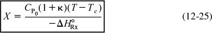
Solving Equation (12-24) for the reactor temperature

Table 12-3 shows three ways to specify the design of a CSTR. This procedure for nonisothermal CSTR design can be illustrated by considering a first-order irreversible liquid-phase reaction. To solve CSTR problems of this type we have three variables X, T, and V and we can only specify two and then solve for the third. The algorithm for working through either cases A (X specified), B (T specified), or C (V specified) is shown in Table 12-3. Its application is illustrated in Example 12-3.
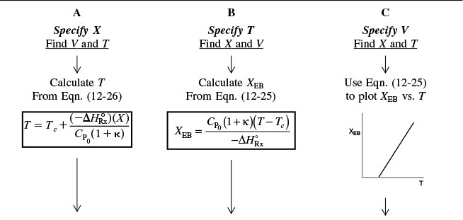
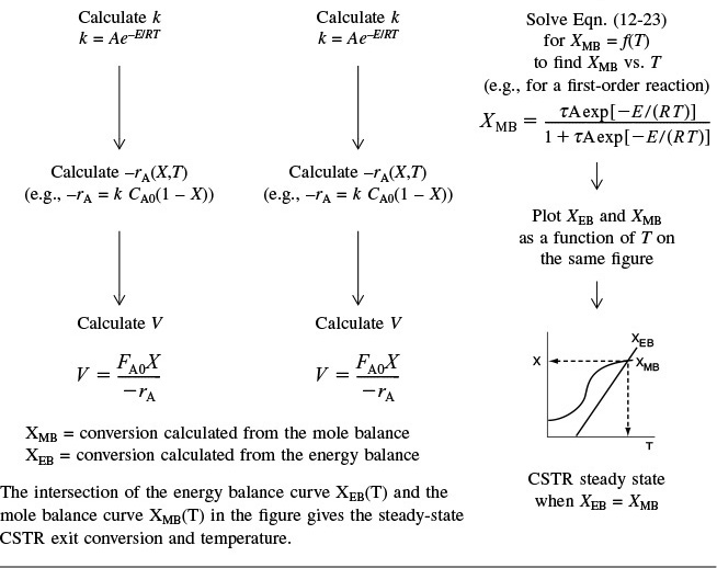
Forms of the energy balance for a CSTR with heat exchange
Example 12–3 Production of Propylene Glycol in an Adiabatic CSTR
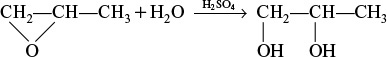
Propylene glycol is produced by the hydrolysis of propylene oxide:
Production, uses, and economics
Over 900 million pounds of propylene glycol were produced in 2010 and the selling price was approximately $0.80 per pound. Propylene glycol makes up about 25% of the major derivatives of propylene oxide. The reaction takes place readily at room temperature when catalyzed by sulfuric acid.
You are the engineer in charge of an adiabatic CSTR producing propylene glycol by this method. Unfortunately, the reactor is beginning to leak, and you must replace it. (You told your boss several times that sulfuric acid was corrosive and that mild steel was a poor material for construction. He wouldn’t listen.) There is a nice-looking, shiny overflow CSTR of 300-gal capacity standing idle; it is glass-lined, and you would like to use it.
We are going to work this problem in lbm, s, ft3, and lb-moles rather than g, mol, and m3 in order to give the reader more practice in working in both the English and metric systems. Many plants still use the English system of units.
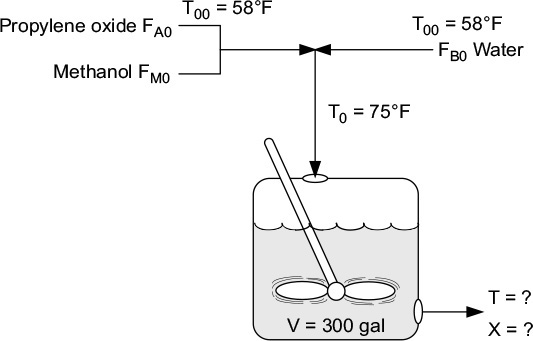
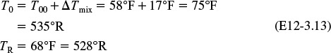
You are feeding 2500 lbm/h (43.04 lb-mol/h) of propylene oxide (P.O.) to the reactor. The feed stream consists of (1) an equivolumetric mixture of propylene oxide (46.62 ft3/h) and methanol (46.62 ft3/h), and (2) water containing 0.1 wt % H2SO4. The volumetric flow rate of water is 233.1 ft3/h, which is 2.5 times the methanol–P.O. volumetric flow rate. The corresponding molar feed rates of methanol and water are 71.87 lb-mol/h and 802.8 lb-mol/h, respectively. The water–propylene oxide–methanol mixture undergoes a slight decrease in volume upon mixing (approximately 3%), but you neglect this decrease in your calculations. The temperature of both feed streams is 58°F prior to mixing, but there is an immediate 17°F temperature rise upon mixing of the two feed streams caused by the heat of mixing. The entering temperature of all feed streams is thus taken to be 75°F (Figure E12-3.1).
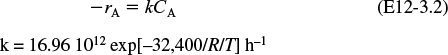
Furusawa et al. state that under conditions similar to those at which you are operating, the reaction is first-order in propylene oxide concentration and apparent zero-order in excess of water with the specific reaction rate4
4 T. Furusawa, H. Nishimura, and T. Miyauchi, J. Chem. Eng. Jpn., 2, 95.
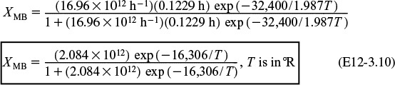
k = Ae–E/RT = 16.96 × 10¹² (e–32,400/RT) h–1
The units of E are Btu/lb-mol and T is in °R.
There is an important constraint on your operation. Propylene oxide is a rather low-boiling-point substance. With the mixture you are using, you feel that you cannot exceed an operating temperature of 125°F, or you will lose too much oxide by vaporization through the vent system.
(a) Can you use the idle CSTR as a replacement for the leaking one if it will be operated adiabatically?
(b) If so, what will be the conversion of propylene oxide to glycol?
Solution
(All data used in this problem were obtained from the CRC Handbook of Chemistry and Physics unless otherwise noted.) Let the reaction be represented by
where
A is propylene oxide (CPA = 35 Btu/lb-mol · °F)5
5 CPA and CPC are estimated from the observation that the great majority of low-molecular-weight oxygen-containing organic liquids have a mass heat capacity of 0.6 cal/g ·°C ±15%.
B is water (CPB = 18 Btu/lb-mol · °F)
C is propylene glycol (CPC = 46 Btu/lb-mol · °F)
M is methanol (CPM = 19.5 Btu/lb-mol · °F)
In this problem, neither the exit conversion nor the temperature of the adiabatic reactor is given. By application of the mole and energy balances, we can solve two equations with two unknowns (X and T), as shown on the right-hand pathway in Table 12-3. Solving these coupled equations, we determine the exit conversion and temperature for the glass-lined reactor to see if it can be used to replace the present reactor.
1. Mole Balance and Design Equation:
FA0 – FA + rAV = 0
The design equation in terms of X is
2. Rate Law:
3. Stoichiometry (liquid phase, υ = υ0):
4. Combining yields
Solving for X as a function of T and recalling that τ = V/υ0 gives
Two equations, two unknowns
This equation relates temperature and conversion through the mole balance.
5. The energy balance for this adiabatic reaction in which there is negligible energy input provided by the stirrer is
This equation relates X and T through the energy balance. We see that two equations, Equations (E12-3.5) and (E12-3.6), and two unknowns, X and T, must be solved (with XEB = XMB = X).
6. Calculations:
Rather than putting all those numbers in the mole and heat balance equations yourself, you can outsource this task to a consulting company in Riça, Jofostan, for a small fee.
(a) Evaluate the mole balance terms (CA0, Θi, τ): The total liquid volumetric flow rate entering the reactor is
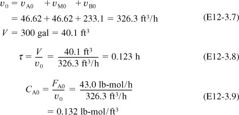

I know these are tedious calculations, but someone’s gotta know how to do it.

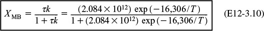
The conversion calculated from the mole balance, XMB, is found from Equation (E12-3.5)
Plot XMB as a function of temperature.
(b) Evaluating the energy balance terms
(1) Heat of reaction at temperature T
ΔCP = CPC – CPB – CPA = 46 – 18 – 35 = –7Btu/lb-mol/°F
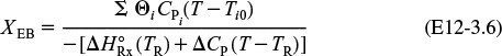
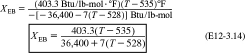
The conversion calculated from the energy balance, XEB, for an adiabatic reaction is given by Equation (11-29)
Substituting all the known quantities into the energy balance gives us
Adiabatic CSTR
7. Solving. There are a number of different ways to solve these two simultaneous algebraic equations (E12-3.10) and (E12-3.14). The easiest way is to use the Polymath nonlinear equation solver. However, to give insight into the functional relationship between X and T for the mole and energy balances, we shall obtain a graphical solution. Here, X is plotted as a function of T for both the mole and energy balances, and the intersection of the two curves gives the solution where both the mole and energy balance solutions are satisfied, i.e., XEB = XMB. In addition, by plotting these two curves we can learn if there is more than one intersection (i.e., multiple steady states) for which both the energy balance and mole balance are satisfied. If numerical root-finding techniques were used to solve for X and T, it would be quite possible to obtain only one root when there is actually more than one. If Polymath were used, you could learn if multiple roots exist by changing your initial guesses in the nonlinear equation solver. We shall discuss multiple steady states further in Section 12-5. We choose T and then calculate X (Table E12-3.1). The calculations for XMB and XEB are plotted in Figure E12-3.2. The virtually straight line corresponds to the energy balance, Equation (E12-3.14), and the curved line corresponds to the mole balance,
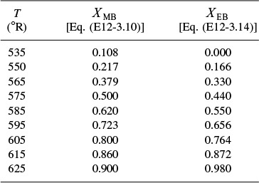
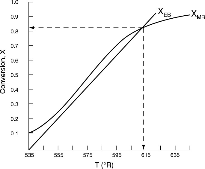
The reactor cannot be used because it will exceed the specified maximum temperature of 585°R.
Equation (E12-3.10). We observe from this plot that the only intersection point is at 83% conversion and 613°R. At this point, both the energy balance and mole balance are satisfied. Because the temperature must remain below 125°F (585°R), we cannot use the 300-gal reactor as it is now.
Analysis: After using Equations (E12-3.10) and (E12-3.14) to make a plot of conversion as a function of temperature, we see that there is only one intersection of XEB(T) and XMB(T), and consequently only one steady state. The exit conversion is 83% and the exit temperature (i.e., the reactor temperature) is 613°R (153°F), which is above the acceptable limit of 585°R (125°F) and we thus cannot use the CSTR operating at these conditions.
Oops! Looks like our plant will not be able to be completed and our multimilliondollar profit has flown the coop. But wait, don’t give up, let’s ask reaction engineer Maxwell Anthony to fly to our company’s plant in the country of Jofostan to look for a cooling coil heat exchanger. See what Max found in Example 12-4.
Example 12–4 CSTR with a Cooling Coil
Fantastic! Max has located a cooling coil in an equipment storage shed in the small, mountainous village of Ölofasis in Jofostan for use in the hydrolsis of propylene oxide discussed in Example 12-3. The cooling coil has 40 ft2 of cooling surface and the cooling-water flow rate inside the coil is sufficiently large that a constant coolant temperature of 85°F can be maintained. A typical overall heat-transfer coefficient for such a coil is 100 Btu/h ·ft2 ·°F. Will the reactor satisfy the previous constraint of 125°F maximum temperature if the cooling coil is used?
Solution
If we assume that the cooling coil takes up negligible reactor volume, the conversion calculated as a function of temperature from the mole balance is the same as that in Example 12-3, Equation (E12-3.10).
1. Combining the mole balance, stoichiometry, and rate law, we have, from Example 12-3
T is in °R.
2. Energy balance. Neglecting the work by the stirrer, we combine Equations (11-27) and (12-20) to write
Solving the energy balance for XEB yields
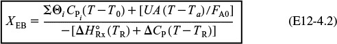
The cooling-coil term in Equation (E12-4.2) is
Recall that the cooling temperature is
Ta = 85°F = 545°R
The numerical values of all other terms of Equation (E12-4.2) are identical to those given in Equation (E12-3.13), but with the addition of the heat exchange term, XEB becomes

We now have two equations, Equations (E12-3.10) and (E12-4.4), and two unknowns, X and T, which we can solve with Polymath. Recall Examples E4-5 and E8-6 to review how to solve nonlinear, simultaneous equations of this type with Polymath. (See Problem P12-1(f) on page 611 to plot X versus T on Figure E12-3.2.)
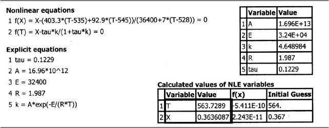
The Polymath program and solution to these two Equations (E12-3.10) for XMB, and (E12-4.4) for XEB, are given in Table E12-4.1. The exiting temperature and conversion are 103.7°F (563.7°R) and 36.4%, respectively, i.e.,
Analysis: We are grateful to the people of the village of Ölofasis in Jofostan for their help in finding this shiny new heat exchanger. By adding heat exchange to the CSTR, the XMB(T) curve is unchanged but the slope of the XEB(T) line in Figure E12-3.2 increases and intersects the XMB curve at X = 0.36 and T = 564°R. This conversion is low! We could try to reduce to cooling by increasing Ta or T0 to raise the reactor temperature closer to 585°R, but not above this temperature. The higher the temperature in this irreversible reaction, the greater the conversion.
We will see in the next section that there may be multiple exit values of conversion and temperature (Multiple Steady States, MSS) that satisfy the parameter values and entrance conditions.
12.5 Multiple Steady States (MSS)
In this section, we consider the steady-state operation of a CSTR in which a first-order reaction is taking place. An excellent experimental investigation that demonstrates the multiplicity of steady states was carried out by Vejtasa and Schmitz.6 They studied the reaction between sodium thiosulfate and hydrogen peroxide
6 S.A. Vejtasa and R. A. Schmitz, AIChE J., 16 (3), 415 (1970).
2Na2S2O3 + 4H2O2 → Na2S3O6 + Na2SO4 + 4H2O
in a CSTR operated adiabatically. The multiple steady-state temperatures were examined by varying the flow rate over a range of space times, τ.
Reconsider the XMB(T) curve, Equation (E12-3.10), shown in Figure E12-3.2, which has been redrawn and shown as dashed lines in Figure E12-3.2A. Now consider what would happen if the volumetric flow rate υ0 is increased (τ decreased) just a little. The energy balance line, XEB(T), remains unchanged, but the mole balance line, XMB, moves to the right, as shown by the curved, solid line in Figure E12-3.2A. This shift of XMB(T) to the right results in the XEB(T) and XMB(T) intersecting three lines, indicating three possible conditions at which the reactor can operate.
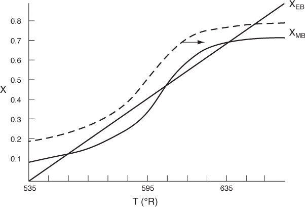
When more than one intersection occurs, there is more than one set of conditions that satisfy both the energy balance and mole balance (i.e., XEB = XMB); consequently, there will be multiple steady states at which the reactor may operate. These three steady states are easily determined from a graphical solution, but only one could show up in the Polymath solution. Thus, when using the Polymath nonlinear equation solver, we need to either choose different initial guesses to find if there are other solutions, or plot XMB and XEB versus T, as in Example 12-3.
We begin by recalling Equation (12-24), which applies when one neglects shaft work and ΔCP (i.e., ΔCP = 0 and therefore ![]() )
)
where
and
Using the CSTR mole balance ![]() , Equation (12-24) may be rewritten as
, Equation (12-24) may be rewritten as
G(T) = Heat-generated term
The left-hand side is referred to as the heat-generated term
The right-hand side of Equation (12-28) is referred to as the heat-removed term (by flow and heat exchange) R(T)
R(T) = Heat-removed term
To study the multiplicity of steady states, we shall plot both R(T) and G(T) as a function of temperature on the same graph and analyze the circumstances under which we will obtain multiple intersections of R(T) and G(T).
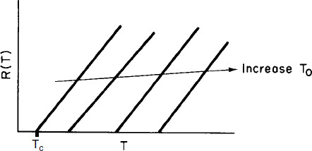
12.5.1 Heat-Removed Term, R(T)
Vary Entering Temperature. From Equation (12-30) we see that R(T) increases linearly with temperature, with slope CP0 (1 + κ) and intercept Tc. As the entering temperature T0 is increased, the line retains the same slope but shifts to the right as the intercept Tc increases, as shown in Figure 12-7.
Vary Non-adiabatic Parameter κ. If one increases κ by either decreasing the molar flow rate, FA0, or increasing the heat-exchange area, A, the slope increases and for the case of Ta < T0 the ordinate intercept moves to the left, as shown in Figure 12-8.


On the other hand, if Ta > T0, the intercept will move to the right as κ increases.
12.5.2 Heat-Generated Term, G(T)
The heat-generated term, Equation (12-29), can be written in terms of conversion. [Recall that X = –rAV/FA0.]
To obtain a plot of heat generated, G(T), as a function of temperature, we must solve for X as a function of T using the CSTR mole balance, the rate law, and stoichiometry. For example, for a first-order liquid-phase reaction, the CSTR mole balance becomes
First-order reaction
Substituting for X in Equation (12-31), we obtain
Finally, substituting for k in terms of the Arrhenius equation, we obtain

Note that equations analogous to Equation (12-33) for G(T) can be derived for other reaction orders and for reversible reactions simply by solving the CSTR mole balance for X. For example, for the second-order liquid-phase reaction
Second-order reaction
the corresponding heat generated term is

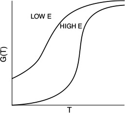
Let’s now examine the behavior of the G(T) curve. At very low temperatures, the second term in the denominator of Equation (12-33) for the first-order reaction can be neglected, so that G(T) varies as
Low T
(Recall that ![]() means that the standard heat of reaction is evaluated at TR.)
means that the standard heat of reaction is evaluated at TR.)
At very high temperatures, the second term in the denominator dominates, and G(T) is reduced to
High T
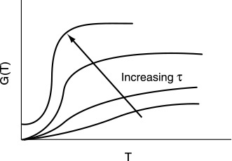
G(T) is shown as a function of T for two different activation energies, E, in Figure 12-9. If the flow rate is decreased or the reactor volume increased so as to increase τ, the heat-generated term, G(T), changes, as shown in Figure 12-10.
Can you combine Figures 12-10 and 12-8 to explain why a Bunsen burner goes out when you turn up the gas flow to a very high rate?
Heat-generated curves, G(T)
12.5.3 Ignition-Extinction Curve
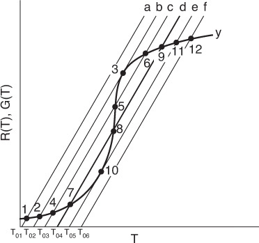
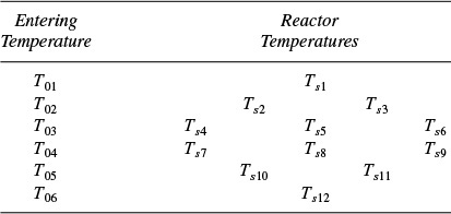
The points of intersection of R(T) and G(T) give us the temperature at which the reactor can operate at steady state. Suppose that we begin to feed our reactor at some relatively low temperature, T01. If we construct our G(T) and R(T) curves, illustrated by curves y = G(T) and a = R(T), respectively, in Figure 12-11, we see that there will be only one point of intersection, point 1. From this point of intersection, one can find the steady-state temperature in the reactor, Ts1, by following a vertical line down to the T-axis and reading off the temperature, Ts1, as shown in Figure 12-11.
If one were now to increase the entering temperature to T02, the G(T) curve, y, would remain unchanged, but the R(T) curve would move to the right, as shown by line b in Figure 12-11, and will now intersect the G(T) at point 2 and be tangent at point 3. Consequently, we see from Figure 12-11 that there are two steady-state temperatures, Ts2 and Ts3, that can be realized in the CSTR for an entering temperature T02. If the entering temperature is increased to T03, the R(T) curve, line c (Figure 12-12), intersects the G(T) curve three times and there are three steady-state temperatures, Ts4, Ts5, and Ts6. As we continue to increase T0, we finally reach line e, in which there are only two steady-state temperatures, a point of tangency at Ts10 and an intersection at Ts11. By further increasing T0, we reach line f, corresponding to T06, in which we have only one reactor temperature that will satisfy both the mole and energy balances, Ts12. For the six entering temperatures, we can form Table 12-4, relating the entering temperature to the possible reactor operating temperatures.
Both the mole and energy balances are satisfied at the points of intersection or tangency.

By plotting Ts as a function of T0, we obtain the well-known ignition-extinction curve shown in Figure 12-13. From this figure, we see that as the entering temperature T0 is increased, the steady-state temperature Ts increases along the bottom line until T05 is reached. Any fraction-of-a-degree increase in temperature beyond T05 and the steady-state reactor temperature Ts will jump up from Ts10 to Ts11, as shown in Figure 12-13. The temperature at which this jump occurs is called the ignition temperature. That is, we must exceed a certain feed temperature, T05, to operate at the upper steady state where the temperature and conversion are higher.

If a reactor were operating at Ts12 and we began to cool the entering temperature down from T06, the steady-state reactor temperature, Ts3, would eventually be reached, corresponding to an entering temperature, T02. Any slight decrease below T02 would drop the steady-state reactor temperature to the lower steady-state value Ts2. Consequently, T02 is called the extinction temperature.
The middle points 5 and 8 in Figures 12-12 and 12-13 represent unstable steady-state temperatures. Consider the heat-removed line d in Figure 12-12, along with the heat-generated curve, which is replotted in Figure 12-14. If we were operating at the middle steady-state temperature Ts8, for example, and a pulse increase in reactor temperature occurred, we would find ourselves at the temperature shown by vertical line ![]() , between points 8 and 9. We see that along this vertical line
, between points 8 and 9. We see that along this vertical line ![]() , the heat-generated curve, y ≡ G(T), is greater than the heat-removed line d ≡ R(T) i.e., (G > R). Consequently, the temperature in the reactor would continue to increase until point 9 is reached at the upper steady state. On the other hand, if we had a pulse decrease in temperature from point 8, we would find ourselves on a vertical line
, the heat-generated curve, y ≡ G(T), is greater than the heat-removed line d ≡ R(T) i.e., (G > R). Consequently, the temperature in the reactor would continue to increase until point 9 is reached at the upper steady state. On the other hand, if we had a pulse decrease in temperature from point 8, we would find ourselves on a vertical line ![]() between points 7 and 8. Here, we see that the heat-removed curve d is greater than the heat-generated curve y (R > G), so the temperature will continue to decrease until the lower steady state is reached. That is, a small change in temperature either above or below the middle steady-state temperature, Ts8, will cause the reactor temperature to move away from this middle steady state. Steady states that behave in this manner are said to be unstable.
between points 7 and 8. Here, we see that the heat-removed curve d is greater than the heat-generated curve y (R > G), so the temperature will continue to decrease until the lower steady state is reached. That is, a small change in temperature either above or below the middle steady-state temperature, Ts8, will cause the reactor temperature to move away from this middle steady state. Steady states that behave in this manner are said to be unstable.
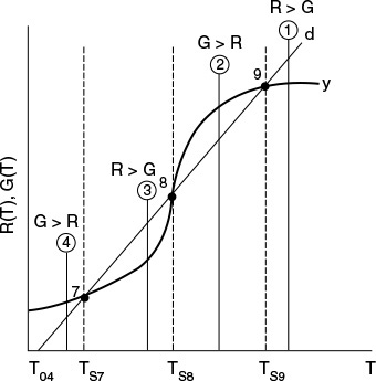
In contrast to these unstable operating points, there are stable operating points. Consider what would happen if a reactor operating at Ts9 were subjected to a pulse increase in reactor temperature indicated by line ![]() in Figure 12-14. We see that the heat-removed line d is greater than the heat-generated curve y (R > G), so that the reactor temperature will decrease and return to Ts9. On the other hand, if there is a sudden drop in temperature below Ts9, as indicated by line
in Figure 12-14. We see that the heat-removed line d is greater than the heat-generated curve y (R > G), so that the reactor temperature will decrease and return to Ts9. On the other hand, if there is a sudden drop in temperature below Ts9, as indicated by line ![]() , we see the heat-generated curve y is greater than the heat-removed line d (G > R), and the reactor temperature will increase and return to the upper steady state at Ts9. Consequently, Ts9 is a stable steady state.
, we see the heat-generated curve y is greater than the heat-removed line d (G > R), and the reactor temperature will increase and return to the upper steady state at Ts9. Consequently, Ts9 is a stable steady state.
Next, let’s look at what happens when the lower steady-state temperature at Ts7 is subjected to pulse increase to the temperature shown as line ![]() in Figure 12-14. Here, we again see that the heat removed, R, is greater than the heat generated, G, so that the reactor temperature will drop and return to Ts7. If there is a sudden decrease in temperature below Ts7 to the temperature indicated by line
in Figure 12-14. Here, we again see that the heat removed, R, is greater than the heat generated, G, so that the reactor temperature will drop and return to Ts7. If there is a sudden decrease in temperature below Ts7 to the temperature indicated by line ![]() , we see that the heat generated is greater than the heat removed (G > R), and that the reactor temperature will increase until it returns to Ts7. Consequently, Ts7 is a stable steady state. A similar analysis could be carried out for temperatures Ts1, Ts2, Ts4, Ts6, Ts11, and Ts12, and one would find that reactor temperatures would always return to locally stable steady-state values when subjected to both positive and negative fluctuations.
, we see that the heat generated is greater than the heat removed (G > R), and that the reactor temperature will increase until it returns to Ts7. Consequently, Ts7 is a stable steady state. A similar analysis could be carried out for temperatures Ts1, Ts2, Ts4, Ts6, Ts11, and Ts12, and one would find that reactor temperatures would always return to locally stable steady-state values when subjected to both positive and negative fluctuations.
While these points are locally stable, they are not necessarily globally stable. That is, a large perturbation in temperature or concentration, while small, may be sufficient to cause the reactor to fall from the upper steady state (corresponding to high conversion and temperature, such as point 9 in Figure 12-14), to the lower steady state (corresponding to low temperature and conversion, point 7).
12.6 Nonisothermal Multiple Chemical Reactions
Most reacting systems involve more than one reaction and do not operate isothermally. This section is one of the most important, if not the most important, sections of the book. It ties together all the previous chapters to analyze multiple reactions that do not take place isothermally.
12.6.1 Energy Balance for Multiple Reactions in Plug-Flow Reactors
In this section we give the energy balance for multiple reactions. We begin by recalling the energy balance for a single reaction taking place in a PFR, which is given by Equation (12-5)

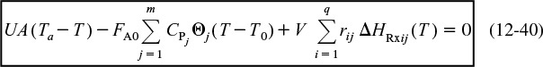
When we have multiple reactions occurring, we have to account for, and sum up, all the heats of reaction in the reactor for each and every reaction. For q multiple reactions taking place in the PFR where there are m species, it is easily shown that Equation (12-5) can be generalized to
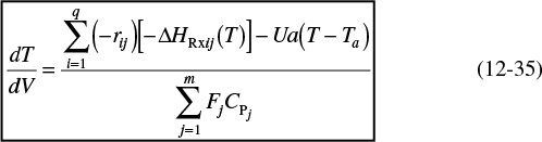
Energy balance for multiple reactions
i = Reaction number
j = Species
Note that we now have two subscripts on the heat of reaction. The heat of reaction for reaction i must be referenced to the same species in the rate, rij, by which ΔHRxij is multiplied, which is

where the subscript j refers to the species, the subscript i refers to the particular reaction, q is the number of independent reactions, and m is the number of species. We are going to let
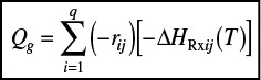
and
Then Equation (12-35) becomes
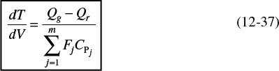
Equation (12-37) represents a nice compact form of the energy balance for multiple reactions.
Consider the following reaction sequence carried out in a PFR:
One of the major goals of this text is that the reader will be able to solve multiple reactions with heat effects, and this section shows how!
The PFR energy balance becomes

![]()
12.6.2 Parallel Reactions in a PFR
We will now give three examples of multiple reactions with heat effects: Example 12-5 discusses parallel reactions, Example 12-6 discusses series reactions, and Example 12-7 discusses complex reactions.
Example 12–5 Parallel Reactions in a PFR with Heat Effects
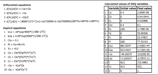
The following gas-phase reactions occur in a PFR:

Pure A is fed at a rate of 100 mol/s, a temperature of 150°C, and a concentration of 0.1 mol/dm3. Determine the temperature and molar flow rate profiles down the reactor.
Additional information
ΔHRx1A = –20,000 J/(mol of A reacted in reaction 1)
ΔHRx2A = –60,000 J/(mol of A reacted in reaction 2)

The PFR energy balance becomes [cf. Equation (12-35)]
1. Mole balances:
2. Rates:
Rate laws
Relative rates

Net rates
3. Stoichiometry (gas-phase but ΔP = 0):


(T in K)
4. Energy balance:
5. Evaluation:
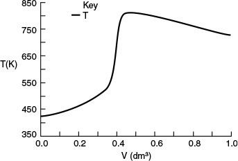
The Polymath program and its graphical outputs are shown in Table E12-5.1 and Figures E12-5.1 and E12-5.2.
Why does the temperature go through a maximum value?
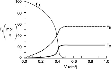
Analysis: The reactant is virtually consumed by the time it reaches a reactor volume V = 0.45 dm3; beyond this point, Qr > Qg, and the reactor temperature begins to drop. In addition, the selectivity ![]() = FB/FC = 55/22.5 = 2.44 remains constant after this point. If a high selectivity is required, then the reactor should be shortened to V = 0.3 dm3, at which point the selectivity is
= FB/FC = 55/22.5 = 2.44 remains constant after this point. If a high selectivity is required, then the reactor should be shortened to V = 0.3 dm3, at which point the selectivity is ![]() = 20/2 = 10.
= 20/2 = 10.
12.6.3 Energy Balance for Multiple Reactions in a CSTR
Recall that for the steady-state mole balance in a CSTR with a single reaction [–FA0X = rAV,] and that ΔHRx(T) = ![]() + ΔCP(T – TR), so that for T0 = Ti0 Equation (11-27) may be rewritten as
+ ΔCP(T – TR), so that for T0 = Ti0 Equation (11-27) may be rewritten as
Again, we must account for the “heat generated” by all the reactions in the reactor. For q multiple reactions and m species, the CSTR energy balance becomes

Energy balance for multiple reactions in a CSTR
Substituting Equation (12-20) for ![]() , neglecting the work term, and assuming constant heat capacities and large coolant flow rates
, neglecting the work term, and assuming constant heat capacities and large coolant flow rates ![]() , Equation (12-39) becomes
, Equation (12-39) becomes
For the two parallel reactions described in Example 12-5, the CSTR energy balance is
Major goal of CRE
One of the major goals of this text is to have the reader solve problems involving multiple reactions with heat effects (cf. Problems P12-23C, P12-24C, P12-25C, and P12-26B). That’s exactly what we are doing in the next two examples!
12.6.4 Series Reactions in a CSTR
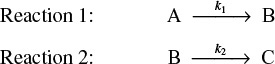
The elementary liquid-phase reactions
take place in a 10-dm3 CSTR. What are the effluent concentrations for a volumetric feed rate of 1000 dm3/min at a concentration of A of 0.3 mol/dm3? The inlet temperature is 283 K.
CPA = CPB = CPC = 200 J/mol · K
k1 = 3.3 min–1 at 300 K, with E1 = 9900 cal/mol
k2 = 4.58 min–1 at 500 K, with E2 = 27,000 cal/mol
ΔHRx1A = –55,000 J/mol A UA = 40,000 J/min ·K with Ta = 57°C
ΔHRx2B = –71,500 J/mol B
Solution
The Algorithm:
Number each reaction

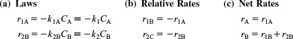
The reactions follow elementary rate laws
r1A = –k1ACA ≡ –k1CA
r2B = –k2BCB ≡ –k2CB
1. Mole Balance on Every Species
Species A: Combined mole balance and rate law for A
Solving for CA gives us
Species B: Combined mole balance and rate law for B
2. Rates
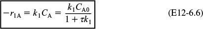
3. Combine
Substituting for r1B and r2B in Equation (E12-6.3) gives
Solving for CB yields
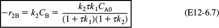
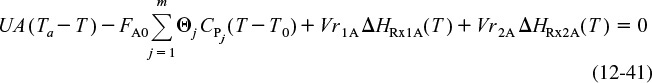
4. Energy Balances:
Applying Equation (12-41) to this system gives
Substituting for FA0 = υ0CA0, r1A, and r2B and rearranging, we have
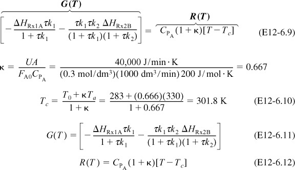
We are going to generate G(T) and R(T) by fooling Polymath to first generate T as a function of a dummy variable, t. We then use our plotting options to convert T(t) to G(T) and R(T). The Polymath program to plot R (T) and G (T) vs. T is shown in Table E12-6.1, and the resulting graph is shown in Figure E12-6.1.
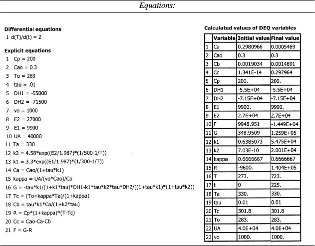
Incrementing temperature in this manner is an easy way to generate R(T) and G(T) plots.
When F = 0, then G(T) = R(T) and the steady states can be found.
Wow! Five (5) multiple steady states!


Analysis: Wow! We see that five steady states (SS) exist!! The exit concentrations and temperatures listed in Table E12-6.2 were determined from the tabular output of the Polymath program. Steady states 1, 3, and 5 are stable steady states, while 2 and 4 are unstable. The selectivity at steady state 3 is ![]() , while at steady state 5 the selectivity is
, while at steady state 5 the selectivity is ![]() and is far too small. Consequently, we either have to operate at steady state 3 or find a different set of operating conditions. What do you think of the value of tau, i.e., τ = 0.01 min? Is it a realistic number?
and is far too small. Consequently, we either have to operate at steady state 3 or find a different set of operating conditions. What do you think of the value of tau, i.e., τ = 0.01 min? Is it a realistic number?
12.6.5 Complex Reactions in a PFR
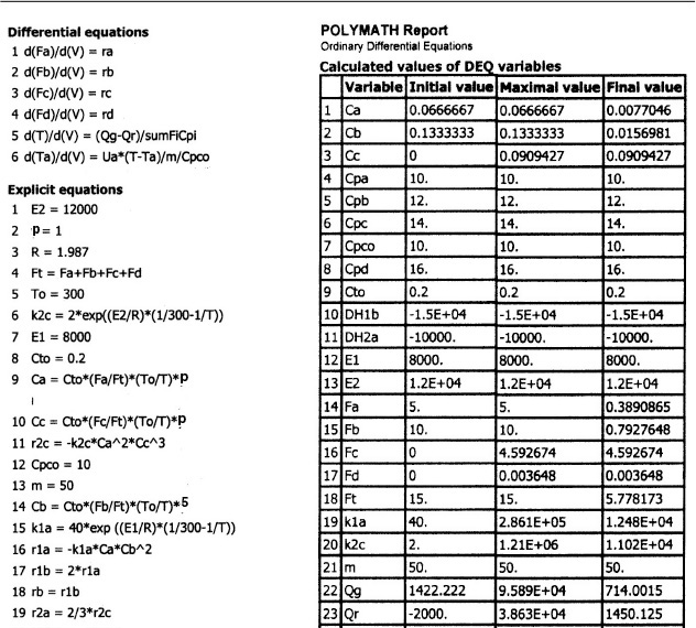
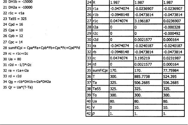
Example 12–7 Complex Reactions with Heat Effects in a PFR
The following complex gas-phase reactions follow elementary rate laws

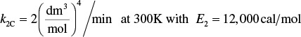
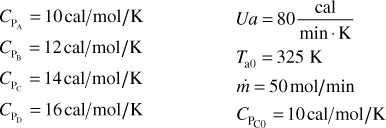
and take place in a PFR. The feed is stoichiometric for reaction (1) in A and B with FA0 = 5 mol/min. The reactor volume is 10 dm3 and the total entering concentration is CT0 = 0.2 mol/dm3. The entering pressure is 100 atm and the entering temperature is 300 K. The coolant flow rate is 50 mol/min and the entering coolant fluid has a heat capacity of CPC0 = 10 cal/mol · K and enters at a temperature of 325 K.
Parameters
Plot FA, FB, FC, FD, p, T, and Ta as a function of V for
(a) Co-current heat exchange
(b) Countercurrent heat exchange
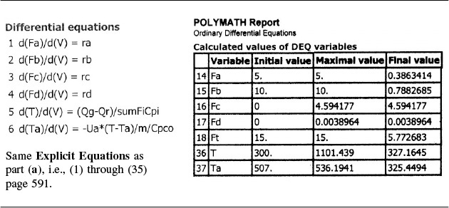
(c) Constant Ta
(d) Adiabatic operation
Solution
Gas Phase PFR No Pressure Drop (p = 1)
1. Mole Balances
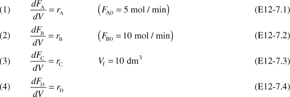
2. Rates:
2a. Rates Law

2b. Relative Rates
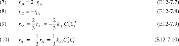
2c. Net Rates of reaction for species A, B, C, and D are
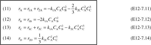
At V = 0, FD = 0 causing SC/D to go to infinity. Therefore, we set SC/D = 0 between V = 0 and a very small number, say, V = 0.0001 dm3 to prevent the ODE solver from crashing.

4. Stoichiometry:
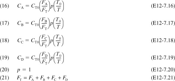
5. Parameters:
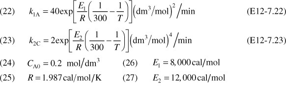
other parameters are given in the problem statement, i.e., Equations (28) to (35) below.

6. Energy Balance:
Recalling Equation (12-37)
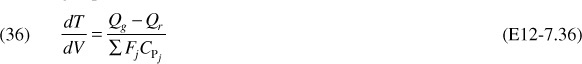
The denominator of Equation (E12-7.36) is
The “heat removed” term is
The “heat generated” is
(a) Co-current heat exchange
The heat exchange balance for co-current exchange is

Part (a) Co-current flow: Plot and analyze the molar flow rates, and the reactor and coolant temperatures as a function of reactor volume.
Co-current heat exchange
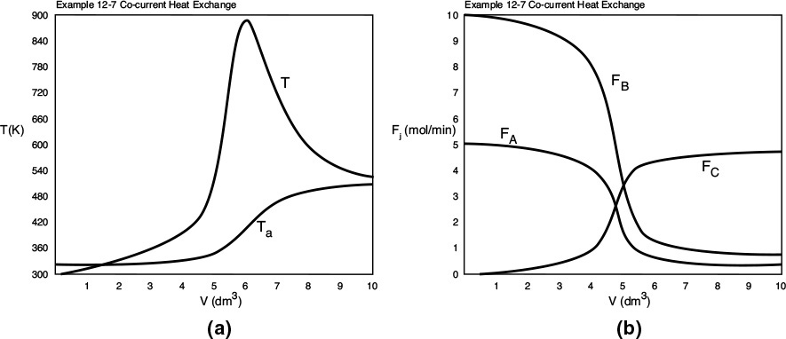
Figure E12-7.1 Profiles for co-current heat exchange; (a) temperature (b) molar flow rates. Note: The molar flow rate FD is very small and is essentially the same as the bottom axis.
Analysis: Part (a): For co-current heat exchange, the selectivity ![]() is really quite good. We also note that the reactor temperature, T, increases when Qg > Qr and reaches a maximum, T = 930 K, at approximately V = 5 dm3. After that, Qr > Qg the reactor temperature decreases and approaches Ta at the end of the reactor.
is really quite good. We also note that the reactor temperature, T, increases when Qg > Qr and reaches a maximum, T = 930 K, at approximately V = 5 dm3. After that, Qr > Qg the reactor temperature decreases and approaches Ta at the end of the reactor.
Part (b) Countercurrent heat exchange: We will use the same program as part (a), but will change the sign of the heat-exchange balance and guess Ta at V = 0 to be 507 K.
We find our guess of 507 K matches Ta0 = 325 K. Are we lucky or what?!
Countercurrent heat exchange

Analysis: Part (b): For countercurrent exchange, the coolant temperature reaches a maximum at V = 1.3 dm3 while the reactor temperature reaches a maximum at V = 2.7 dm3. The reactor with a countercurrent exchanger reaches a maximum reactor temperature of 1100 K, which is greater than that for the co-current exchanger, (i.e., 930 K). Consequently, if there is a concern about additional side reactions occurring at this maximum temperature of 1100 K, one should use a co-current exchanger or maintain constant Ta in the exchanger. In Figure 12-7.2(a) we see that the reactor temperature approaches the coolant entrance temperature at the end of the reactor. The selectivity for the countercurrent systems, ![]() , is slightly lower than that for the co-current exchange.
, is slightly lower than that for the co-current exchange.
Part (c) Constant Ta: To solve the case of constant heating-fluid temperature, we simply multiply the right-hand side of the heat-exchanger balance by zero, i.e.,
and use Equations (E12-7.1) through (E12-7.40).

Constant Ta
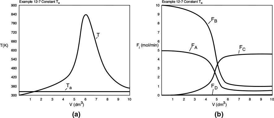
Analysis: Part (c): For constant Ta, the maximum reactor temperature, 870K, is less than either co-current or countercurrent exchange while the selectivity, ![]() , is greater than either co-current or countercurrent exchange. Consequently, one should investigate how to achieve sufficiently high mass flow of the coolant in order to maintain constant Ta.
, is greater than either co-current or countercurrent exchange. Consequently, one should investigate how to achieve sufficiently high mass flow of the coolant in order to maintain constant Ta.
Part (d) Adiabatic: To solve for the adiabatic case, we simply multiply the overall heat transfer coefficient by zero.
Ua = 80 * 0
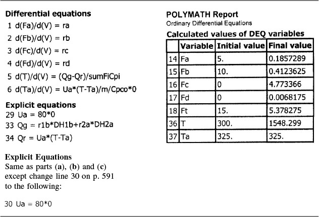
Adiabatic operation
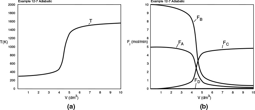
Analysis: Part (d): For the adiabatic case, the maximum temperature, which is the exit temperature, is higher than the other three exchange systems, and the selectivity is the lowest. At this high temperature, the occurrence of unwanted side reactions certainly is a concern.
Overall Analysis Parts (a) to (d): Suppose the maximum temperature in each of these cases is outside the safety limit of 750 K for this system. Problem P12-2A (h) asks how you can keep the maximum temperature below 750 K.
12.7 Radial and Axial Variations in a Tubular Reactor
In the previous sections, we have assumed that there were no radial variations in velocity, concentration, temperature, or reaction rate in the tubular and packed-bed reactors. As a result, the axial profiles could be determined using an ordinary differential equation (ODE) solver. In this section, we will consider the case where we have both axial and radial variations in the system variables, in which case we will require a partial differential (PDE) solver. A PDE solver such as COMSOL will allow us to solve tubular reactor problems for both the axial and radial profiles, as shown in the Radial Effects COMSOL Web module on the CRE Web site (http://www.umich.edu/~elements/5e/web_mod/radialeffects/index.htm.7 In addition, a number of COMSOL examples associated with and developed for this book are available from the COMSOL Web site (www.comsol.com/ecre).
7 An introductory webinar on COMSOL can be found on the AIChE webinar Web site: http://www.aiche.org/resources/chemeondemand/webinars/modeling-non-ideal-reactors-and-mixers.
COMSOL application

We are going to carry out differential mole and energy balances on the differential cylindrical annulus shown in Figure 12-15.
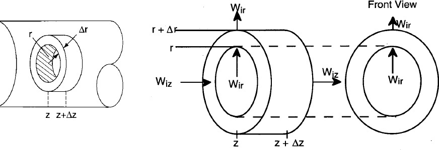
12.7.1 Molar Flux
In order to derive the governing equations, we need to define a couple of terms. The first is the molar flux of species i, Wi (mol/m2 · s). The molar flux has two components, the radial component, Wir, and the axial component, Wiz. The molar flow rates are just the product of the molar fluxes and the cross-sectional areas normal to their direction of flow Acz. For example, for species i flowing in the axial (i.e., z) direction
Fiz = WizAcz
where Wiz is the molar flux in the z direction (mol/m2/s), and Acz (m2) is the cross-sectional area of the tubular reactor.
In Chapter 14 we discuss the molar fluxes in some detail, but for now let us just say they consist of a diffusional component, –De(∂Ci/∂z), and a convective flow component, UzCi
where De is the effective diffusivity (or dispersion coefficient) (m2/s), and Uz is the axial molar average velocity (m/s). Similarly, the flux in the radial direction is
Radial direction
where Ur (m/s) is the average velocity in the radial direction. For now, we will neglect the velocity in the radial direction, i.e., Ur = 0. A mole balance on species A (i.e., i = A) in a cylindrical system volume of length Δz and thickness Δr as shown in Figure 12-15 gives
Mole Balances on Species A
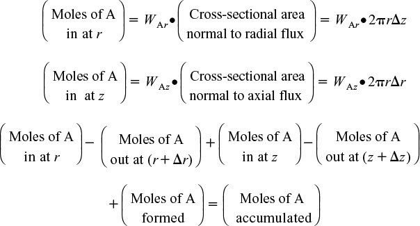

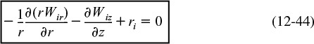
Dividing by 2πrΔrΔz and taking the limit as Δr and Δz → 0
Similarly, for any species i and steady-state conditions
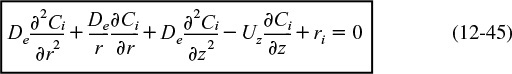
Using Equations (12-42) and (12-43) to substitute for Wiz and Wir in Equation (12-44) and then setting the radial velocity to zero, Ur = 0, we obtain
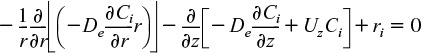
For steady-state conditions and assuming Uz does not vary in the axial direction
This equation will also be discussed further in Chapter 17.
12.7.2 Energy Flux
When we applied the first law of thermodynamics to a reactor to relate either temperature and conversion or molar flow rates and concentration, we arrived at Equation (11-10). Neglecting the work term we have for steady-state conditions
In terms of the molar fluxes and the cross-sectional area, and (q = ![]() /Ac)
/Ac)
The q term is the heat added to the system and almost always includes a conduction component of some form. We now define an energy flux vector, e, (J/m2 · s), to include both the conduction and convection of energy.
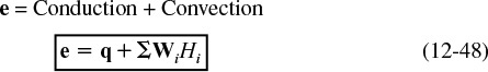
e = energy flux vector J/s · m2
where the conduction term q (kJ/m2 · s) is given by Fourier’s law. For axial and radial conduction, Fourier’s laws are
where ke is the thermal conductivity (J/m·s·K). The energy transfer (flow) is the flux vector times the cross-sectional area, Ac, normal to the energy flux
Energy flow = e · Ac
12.7.3 Energy Balance
Using the energy flux, e, to carry out an energy balance on our annulus (Figure 12-15) with system volume 2πrΔrΔz, we have

(er2πrΔz)|r – (er2πrΔz)|r+ Δr + ez 2πrΔr|z – ez 2πrΔr|z+ Δz = 0
Dividing by 2πrΔrΔz and taking the limit as Δr and Δz → 0
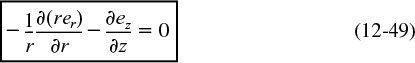
The radial and axial energy fluxes are
er = qr + ΣWirHi
ez = qz + ΣWizHi
Substituting for the energy fluxes, er and ez
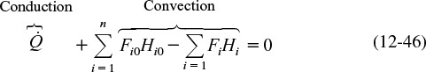
and expanding the convective energy fluxes, ΣWi Hi,
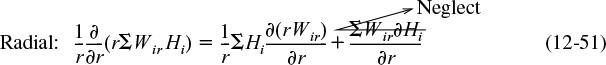
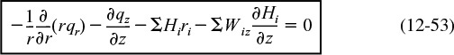
Substituting Equations (12-51) and (12-52) into Equation (12-50), we obtain upon rearrangement

Recognizing that the term in brackets is related to Equation (12-44) and is just the rate of formation of species i, ri, for steady-state conditions we have
Recalling
and
ri = vi(–rA)
ΣriHi = ΣviHi(–rA) = –ΔHRxrA
we have the energy in the form
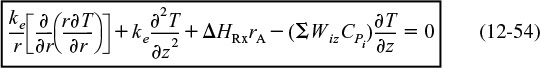
where Wiz is given by Equation (12-42). Equation (12-54) would be coupled with the mole balance, rate law, and stoichiometric equations to solve for the radial and axial concentration at gradients. However, a great amount of computing time would be required. Let’s see if we can make some approximations to simplify the solution.
Some Initial Approximations
Assumption 1. Neglect the diffusive term, wrt, the convective term in Equation (12-42) in the expression involving heat capacities
ΣCPiWiz = ΣCPi(0 + UzCi) = ΣCPiCiUz
With this assumption, Equation (12-54) becomes
For laminar flow, the velocity profile is
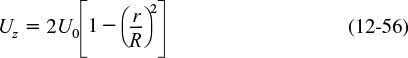
where U0 is the average velocity inside the reactor.
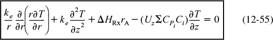
Assumption 2. Assume that the sum CPm = ΣCPiCi = CA0ΣΘiCPi is constant. The energy balance now becomes
Energy balance with radial and axial gradients
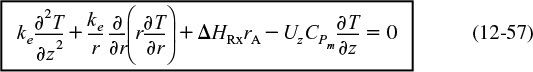
Equation (12-56) is the form we will use in our COMSOL problem. In many instances, the term CPm is just the product of the solution density (kg/m3) and the heat capacity of the solution (kJ/kg · K).
Coolant Balance
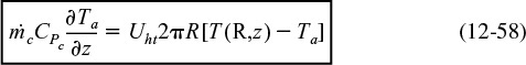
We also recall that a balance on the coolant gives the variation of coolant temperature with axial distance where Uht is the overall heat transfer coefficient and R is the reactor wall radius
Boundary and Initial Conditions
A. Initial conditions if other than steady state (not considered here) t = 0, Ci = 0, T = T0, for z > 0 all r
B. Boundary conditions
1) Radial
(a) At r = 0, we have symmetry ∂T/∂r = 0 and ∂Ci/∂r = 0.
(b) At the tube wall, r = R, the temperature flux to the wall on the reaction side equals the convective flux out of the reactor into the shell side of the heat exchanger.
(c) There is no mass flow through the tube walls ∂Ci/∂r = 0 at r = R.
2) Axial
(a) At the entrance to the reactor z = 0
T = T0 and Ci = Ci0
(b) At the exit of the reactor z = L
The preceding equations were used to describe and analyze flow and reaction in a tubular reactor with heat exchange as described in the following example, which can be found in the Expanded Material on the CRE Web site. What follows is only a brief outline of that example with a few results from the output of the COMSOL program.
Example W12–8 Tubular reactor with axial and radial gradients.
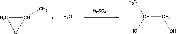
The liquid phase reaction was analyzed using COMSOL to study both axial and radial variations, and the details can be found on the home page of the CRE Web site, www.umich.edu/~elements/5e/index.html, by clicking on the Expanded Material for Chapter 12. Typical temperature profiles for this example are shown in Figures 12-16 and 12-17.
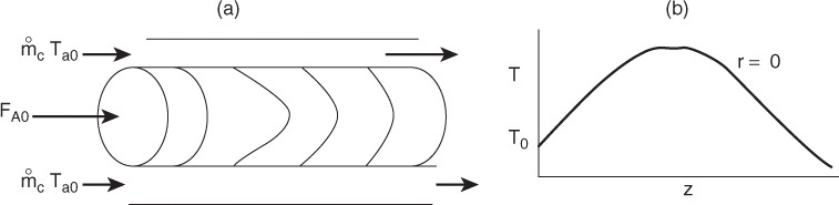
Results
Results of the COMSOL simulation
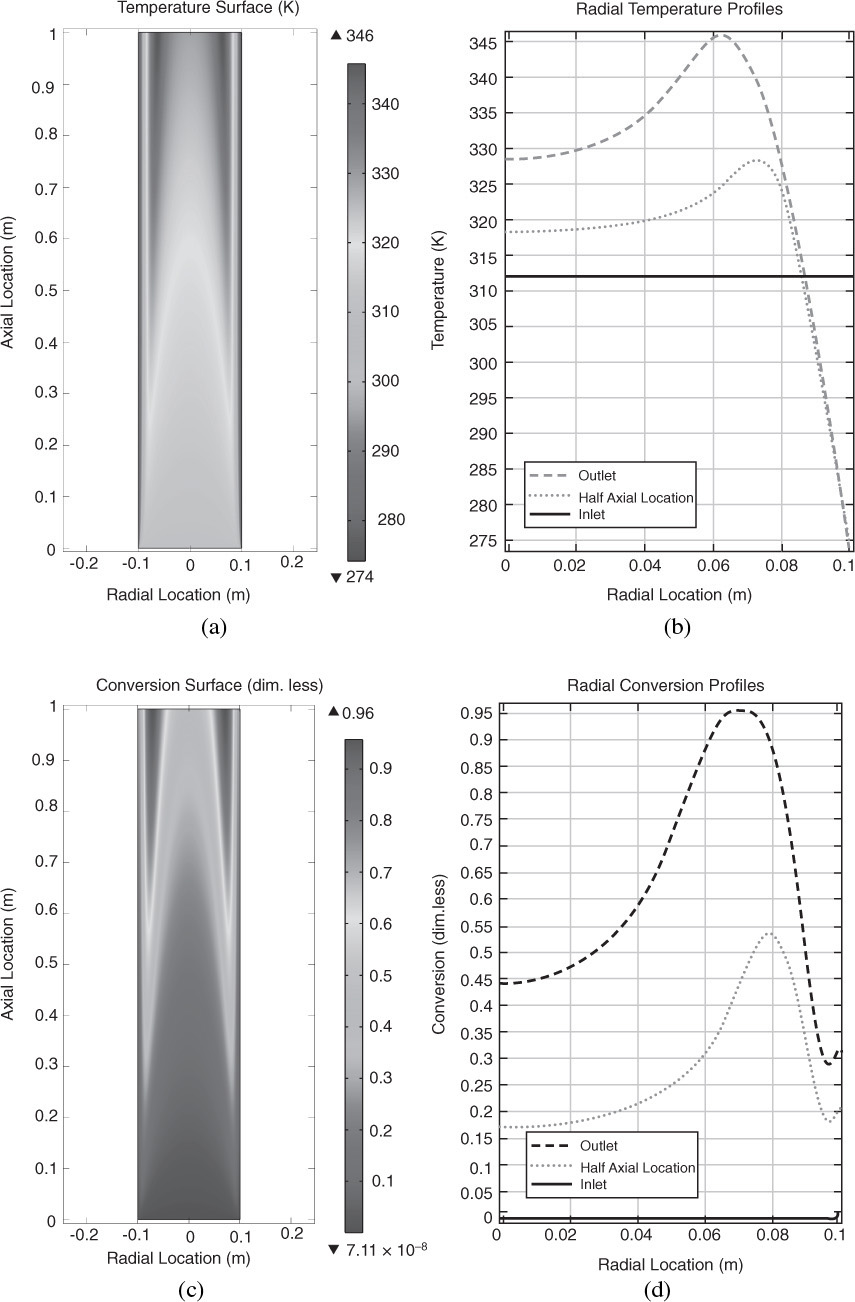
Figure 12-17 (a) Temperature surface, (b) temperature surface profiles, (c) conversion surface, and (d) radial profile. (Continues)
The volumetric flow rate of water is 3.5 times the volumetric flow rate of the mixture of propylene oxide in methanol.
Analysis: One notes from the temperature surface plot that the temperature is set to 312 K at the entrance and that it rapidly decreases along the walls with the distance from the inlet. These same profiles can be found in color on the CRE Web site in the Web Modules. Be sure to note the predicted maximum and minimum in the temperature and concentration profiles. Near the wall, the temperature of the mixture is lower because of the cold wall temperature, which is cooled by the jacket. Consequently, the reaction rate will be lower, and thus the conversion will be lower. However, right next to the wall, the flow velocity through the reactor is almost zero, due to the friction with the wall, so the reactants spend a long time in the reactor; therefore, a greater conversion is achieved, as noted by the upturn right next to the wall.
COMSOL Web Site
Examples can be found on the COMSOL Web site (www.comsol.com/ecre), including the radial effects in tubular reactor examples: Isothermal Reactor, Nonisothermal Adiabatic Reactor, Nonisothermal Reactor with Isothermal Cooling Jacket, and Nonisothermal Reactor with Variable Coolant Temperature. You can also access the Tubular Reactor app directly from the Web site. This app solves the equations defined in the Nonisothermal Reactor with Variable Coolant Temperature exercise, which is embedded in the app. In these examples, you are also in the Living Example Program format (LEP). In accessing these LEPs, make sure that you either have COMSOL installed on your laptop or that it is available on your university computer. On the COMSOL Web site, www.comsol.com/ecre, you can also find how to locate the LEPs in the installed COMSOL Application Libraries.
Also, other applications based on exercises from this book are found at the COMSOL Web site (www.comsol.com/ecre). These include the following applications: activation_energy based on the example Determination of Activation Energy in this book; cstr_startup from the exercise Startup of a CSTR; non_ideal_cstr based on the paragraph Real CSTR Modeled as Two CSTRs with Interchange; and non_isothermal_plug_flow based on the example Production of Acetic Anhydride.
12.8 Safety
Scaling up exothermic chemical reactions can be very tricky. Tables 12-5 and 12-6 give reactions that have resulted in accidents and their causes, respectively.8 The reader should review the case histories of these reactions to learn how to avoid similar accidents.
8 Courtesy of J. Singh, Chemical Engineering, 92 (1997) and B. Venugopal, Chemical Engineering, 54 (2002).

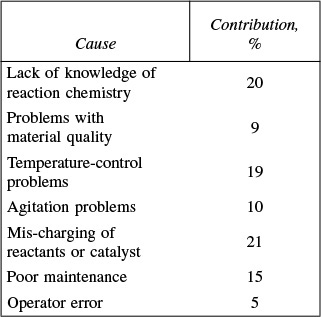
Runaway reactions are the most dangerous in reactor operation, and a thorough understanding of how and when they could occur is part of the chemical reaction engineer’s responsibility. The reaction in the last example in this chapter could be thought of as running away. Recall that as we moved down the length of the reactor, none of the cooling arrangements could keep the reactor from reaching an extremely high temperature (e.g., 800 K). In the next chapter, we study case histories of two runaway reactions. One is the nitroaniline explosion discussed in Example E13-2 and the other is Example E13-6, concerning the recent (2007) explosion at T2 Laboratories. (http://www.chemsafety.gov/videoroom/detail.aspx?VID=32).
There are many resources available for additional information on reactor safety and the management of chemical reactivity hazards. Guidelines for managing chemical reactivity hazards and other fire, explosion, and toxic release hazards are developed and published by the Center for Chemical Process Safety (CCPS) of the American Institute of Chemical Engineers. CCPS books and other resources are available at www.aiche.org/ccps. For example, the book Essential Practices for Managing Chemical Reactivity Hazards, written by a team of industry experts, is also provided free of charge by CCPS on the site www.info.knovel.com/ccps. A concise and easy-to-use software program that can be used to determine the reactivity of substances or mixtures of substances, the Chemical Reactivity Worksheet, is provided by the National Oceanic and Atmospheric Administration (NOAA) for free on its Web site, www.noaa.gov.
The Safety and Chemical Engineering Education (SAChE) program was formed in 1992 as a cooperative effort between the AIChE, CCPS, and engineering schools to provide teaching materials and programs that bring elements of process safety into the education of undergraduate and graduate students studying chemical and biochemical products and processes. The SAChE Web site (www.sache.org) has a great discussion of reactor safety with examples as well as information on reactive materials. These materials are also suitable for training purposes in an industrial setting.
The following instruction modules are available on the SAChE Web site (www.sache.org).
1. Chemical Reactivity Hazards: This Web-based instructional module contains about 100 Web pages with extensive links, graphics, videos, and supplemental slides. It can be used either for classroom presentation or as a self-paced tutorial. The module is designed to supplement a junior or senior chemical engineering course by showing how uncontrolled chemical reactions in industry can lead to serious harm, and by introducing key concepts for avoiding unintended reactions and controlling intended reactions.
2. Runaway Reactions: Experimental Characterization and Vent Sizing: This instruction module describes the ARSST and its operation, and illustrates how this instrument can easily be used to experimentally determine the transient characteristics of runaway reactions, and how the resulting data can be analyzed and used to size the relief vent for such systems.
3. Rupture of a Nitroaniline Reactor: This case study demonstrates the concept of runaway reactions and how they are characterized and controlled to prevent major losses.
4. Seveso Accidental Release Case History: This presentation describes a widely discussed case history that illustrates how minor engineering errors can cause significant problems; problems that should not be repeated. The accident was in Seveso, Italy, in 1976. It was a small release of a dioxin that caused many serious injuries.
Membership in SAChE is required to view these materials. Virtually all U.S. universities and many non-U.S universities are members of SAChE—contact your university SAChE representative, listed on the SAChE Web site, or your instructor or department chair to learn your university’s username and password. Companies can also become members—see the SAChE Web site for details.
Note: Access is restricted to SAChE members and universities
Certificate Program
SAChE also offers several certificate programs that are available to all chemical engineering students. Students can study the material, take an online test, and receive a certificate of completion. The following two certificate programs are of value for reaction engineering:
1. Runaway Reactions: This certificate focuses on managing chemical reaction hazards, particularly runaway reactions.
2. Chemical Reactivity Hazards: This is a Web-based certificate that provides an overview of the basic understanding of chemical reactivity hazards.
Many students are taking the certificate test online and put the fact that they successfully obtained the certificate on their résumés.
More information on safety is given in the Summary Notes and Professional Reference Shelf on the Web. Particularly study the use of the ARSST to detect potential problems. These will be discussed in Chapter 13 Professional Reference Shelf R13.1 on the CRE Web site.

In terms of conversion
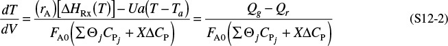
2. The temperature dependence of the specific reaction rate is given in the form

3. The temperature dependence of the equilibrium constant is given by van’t Hoff’s equation for ΔCP = 0
4. Neglecting changes in potential energy, kinetic energy, and viscous dissipation, and for the case of no work done on or by the system, large coolant flow rates (![]() ), and all species entering at the same temperature, the steady-state CSTR energy balance for single reactions is
), and all species entering at the same temperature, the steady-state CSTR energy balance for single reactions is
5. Multiple steady states

where ![]() and
and ![]()

6. When q multiple reactions are taking place and there are m species

7. Axial or radial temperature and concentration gradients. The following coupled, partial differential equations were solved using COMSOL:
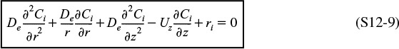
and
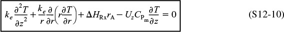
CRE Web Site Materials
• Expanded Material
1. COSMOL Example W12-8
2. Problems
COMSOL LEP W12-8
WP12-18C
WP12-21B
WP12-24B
WP12-31B
• Learning Resources
1. Summary Notes
2. Web Module COMSOL Radial and Axial Gradients
3. Interactive Computer Games (ICGs)
A. Heat Effects I
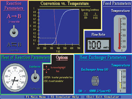
B. Heat Effects II
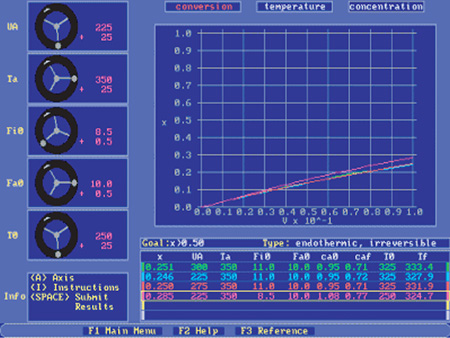
A. Example 12-2 Formulated in AspenTech: Download AspenTech directly from the CRE Web site.
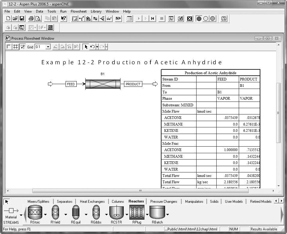
A step-by-step AspenTech tutorial is given on the CRE Web site.
B. Example CD12-1 ΔHRx(T) for Heat Capacities Expressed as Quadratic Functions of Temperature
C. Example CD12-2 Second-Order Reaction Carried Out Adiabatically in a CSTR
5. PFR/PBR Solution Procedure for a Reversible Gas-Phase Reaction
• Living Example Problems
1. Example 12-1 Isomerization of Normal Butane with Heat Exchange
2. Example 12-2 Production of Acetic Anhydride
3. Example 12-2Asp AspenTech Formulation
4. Example 12-4 CSTR with Cooling Coil
5. Example 12-5 Parallel Reaction in a PFR with Heat Effects
6. Example 12-6 Multiple Reactions in a CSTR
7. Example 12-7 Complex Reactions
8. Example W12-8 COSMOL Radial Effects in a Tubular Reactor
9. Example R12-1 Industrial Oxidation of SO2
10. Example 12-T12-3 PBR with Variable Coolant Temperature, Ta
• Professional Reference Shelf
R12.1. Runaway in CSTRs and Plug-Flow Reactors
Phase Plane Plots. We transform the temperature and concentration profiles into a phase plane.
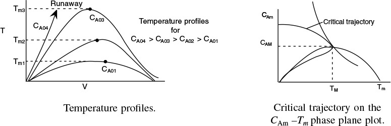
The trajectory going through the maximum of the “maxima curve” is considered to be critical and therefore is the locus of the critical inlet conditions for CA and T corresponding to a given wall temperature.
R12.2. Steady-State Bifurcation Analysis. In reactor dynamics, it is particularly important to find out if multiple stationary points exist or if sustained oscillations can arise.
R12.3. Heat Capacity as a Function of Temperature. Combining the heat of reaction with the quadratic form of the heat capacity
CPi = αi + βiT + γiT2
we find that

Example 12-2 is reworked on the PRS for the case of variable heat capacities.
R12.4. Manufacture of Sulfuric Acid. The details of the industrial oxidation of SO2 are described. Here, the catalyst quantities, the reactor configuration, and operating conditions are discussed, along with a model to predict the conversion and temperature profiles.
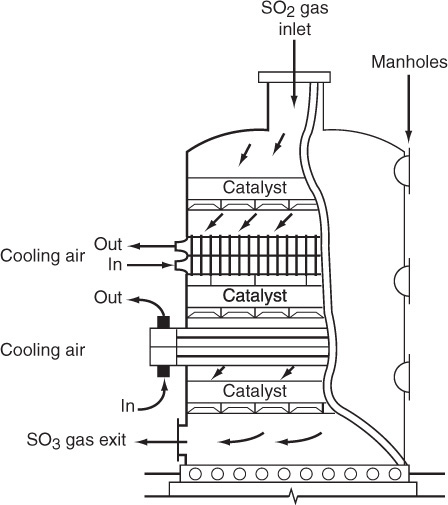
Questions and Problems

The subscript to each of the problem numbers indicates the level of difficulty: A, least difficult; D, most difficult.
In each of the questions and problems, rather than just drawing a box around your answer, write a sentence or two describing how you solved the problem, the assumptions you made, the reasonableness of your answer, what you learned, and any other facts that you want to include. See Preface Section I for additional generic parts (x), (y), and (z) to the home problems.
Before solving the problems, state or sketch qualitatively the expected results or trends.
Questions
Q12-1A Review Figure 12-13. Use this figure to write a few sentences (or at least draw on analogy) explaining why, when you strike the head of a safety match slowly on its pumice with little pressure, it may heat up a little, but does not ignite, yet when you put pressure on it and strike it rapidly, it does ignite. Thanks to Oscar Piedrahita, Medellín, Colombia.

Q12-2A Read over the problems at the end of this chapter. Make up an original problem that uses the concepts presented in this chapter. To obtain a solution:
(a) Make up your data and reaction.
(b) Use a real reaction and real data. See Problem P5-1A for guidelines.
(c) Prepare a list of safety considerations for designing and operating chemical reactors. (See www.sache.org and www.siri.org/graphics.) The August 1985 issue of Chemical Engineering Progress may be useful for part (c).
Problems
We will use the Living Example on the CRE Web site extensively to carry out simulations. Why carry out simulations to vary the parameters in the Living Example Problems? We do it in order to
• Get a more intuitive feel reactor system.
• Gain insight about the most sensitive parameters (e.g., E, KC) and how they affect outlet conditions.
• Learn how reactors are affected by different operating conditions.
• Simulate dangerous situations such as potential runaway reactions.
• Compare the model and parameters with experimental data.
• Optimize the reaction system.
P12-1A Download the following Polymath programs (i.e., LEPs) from the CRE Web site where appropriate. In addition to the LEPs having Polymath and MATLAB codes, some LEPs have Wolfram. Previous students suggest using Wolfram to save time in working through the parameter variation problems to understand how the reactor behaves when parameters are varied.
(a) Example 12-1. Safety. Suppose the value of the equilibrium constant and heat of reaction were measured incorrectly and were found to be KC = 1,000 mol/dm3 at 330 K and ΔHRx = –20,000 kJ/mol. (1) Redo Example 12-1 using these values. (2) Let Qg = rAΔHRx and Qr = Ua (T – Ta), and then plot Qg and Qr on the same figure as a function of V. (3) Vary the coolant flow rate (0 < ![]() < 2,000 kg/h) and the entering temperature 273 (K < T0 < 315 K), and describe what you find. (4) Vary some of the other parameters and see if you can find unsafe operating conditions. (5) Plot Qr and Ta as a function of V necessary to maintain isothermal operation.
< 2,000 kg/h) and the entering temperature 273 (K < T0 < 315 K), and describe what you find. (4) Vary some of the other parameters and see if you can find unsafe operating conditions. (5) Plot Qr and Ta as a function of V necessary to maintain isothermal operation.
(b) Example 12-2 (Use the LEP). (1) Let Qg = rAΔHRx and Qr = Ua (T – Ta), and then plot Qg and Qr on the same figure as a function of V. (2) Fix the reactor volume at 0.5 m3 and the entrance conditions at (T0 = 1050 K, Ta0 = 1250 K), and then make a table, Xe, X, Ta, and T for each of the heat exchange cases. Change the inlet conditions and determine which heat exchanger case gives the greatest differences in the conversion. (3) Repeat (2) for V = 5 m3. (4) Plot Qg, Qr, and –rA versus V for all four cases on the same figure and describe what you find. (5) For each of the four heat exchanger cases, investigate the addition of an inert I with a heat capacity of 50 J/mol · K, keeping FA0 constant and letting the other inlet conditions adjust accordingly (e.g., ε). (6) Vary the inert molar flow rate (i.e., ΘI, 0.0 < ΘI < 3.0 mol/s). Plot X and analyze versus ΘI. (7) Finally, vary the heat-exchange fluid temperature Ta0 (1,000°F < Ta0 < 1350°F). Write a paragraph describing what you find, noting interesting profiles or results.

(c) Example 12-2. AspenTech Formulation. Repeat P12-2(b) using AspenTech.
(d) Problem 12-3B Solution. Load the LEP for this problem and answer the questions in P12-3B. Students have pointed out that using Wolfram can greatly speed the solutions to the various parts of this problem.
(e) Example 12-3 (Use the LEP). Describe how your answers would change if the molar flow rate of methanol were increased by a factor of 4.
(f) Example 12-4 (Use the LEP). (1) Use Figure E12-3.2 and Equation (E12-4.4) to plot X versus T to find the new exit conversion and temperature. (2) Other data show ![]() and CPA = 29 Btu/lb-mol/°F. How would these values change your results? (3) Make a plot of conversion as a function of heat exchanger area. [0 < A < 200 ft2].
and CPA = 29 Btu/lb-mol/°F. How would these values change your results? (3) Make a plot of conversion as a function of heat exchanger area. [0 < A < 200 ft2].
(g) Example 12-5 (Use the LEP). (1) Why is there a maximum in temperature? How would your results change if there is (2) a pressure drop with α = 1.05 dm–3? (3) Reaction (1) is reversible with KC = 10 at 450 K? (4) How would the selectivity change if Ua is increased? Decreased?
(h) Example 12-6 (Use the LEP). (1) Vary T0 to make a plot of the reactor temperature, T, as a function of T0. What are the extinction and ignition temperatures? (2) Vary τ between 0.1 min and 0.001 min and describe what you find. (3) Vary Ua between 4,000 and 400,000 J/min/K and describe what you find.
(i) Example 12-7 (Use the LEP). (1) Safety. Plot Qg and Qr as a function of V. How can you keep the maximum temperature below 700 K? Would adding inerts help and if so what should the flow rate be if CPI = 10 cal/mol/K? (2) Look at the Figures. What happened to species D? What conditions would you suggest to make more species D? (3) Make a table of the temperature (e.g., maximum T, Ta) and molar flow rates at two or three volumes, comparing the different heat-exchanger operations. (4) Why do you think the molar flow rate of C does not go through a maximum? Vary some of the parameters to learn if there are conditions where it goes through a maximum. Start by increasing FA0 by a factor of 5. (5) Include pressure in this problem. Vary the pressure-drop parameter (0 < αρb < 0.0999 dm–3) and describe what you find.
(j) CRE Web site SO2 Example PRS-R12.4-1. Download the SO2 oxidation LEP R12-1. How would your results change if (1) the catalyst particle diameter were cut in half? (2) The pressure were doubled? At what particle size does pressure drop become important for the same catalyst weight, assuming the porosity doesn’t change? (3) You vary the initial temperature and the coolant temperature? Write a paragraph describing what you find.
(k) SAChE. Go to the SAChE Web site, www.sache.org. Your instructor or department chair should have the username and password to enter the SAChE Web site in order to obtain the modules with the problems. On the left-hand menu, select “SAChE Products.” Select the “All” tab and go to the module entitled, “Safety, Health and the Environment” (S, H & E). The problems are for KINETICS (i.e., CRE). There are some example problems marked “K” and explanations in each of the above S, H & E selections. Solutions to the problems are in a different section of the site. Specifically look at: Loss of Cooling Water (K-1), Runaway Reactions (HT-1), Design of Relief Values (D-2), Temperature Control and Runaway (K-4) and (K-5), and Runaway and the Critical Temperature Region (K-7). Go through the K problems and write a paragraph on what you have learned.
(l) COMSOL Homework Problem (LEP). There is a COMSOL problem in the Expanded Material on the CRE Web site (www.comsol.com/ecre).
P12-2A Use Wolfram LEP to find the value of ΘB that would be required to not allow reactor temperature to rise above 360 K?
P12-3B Load Polymath or Wolfram or MATLAB for LEP 12-T12-3 for Table T12-2 from the CRE Web site for this exothermic reversible reaction with a variable coolant flow rate.
has the following parameter values for the base case:
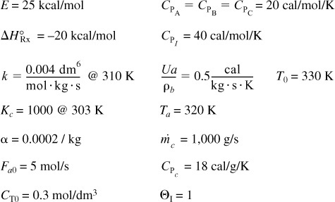
Vary the following parameters in the ranges shown in parts (a) through (i). Write a paragraph describing the trends you find for each parameter variation and why they look the way they do. Use the base case for parameters not varied. Hint: See ![]() and
and ![]() at the very end of the Chapter 12 Summary Notes on the CRE Web site. The feedback from students on this problem is that one should use Wolfram in the LEP 12-3 on the Web to carry out the parameter variations. Note: Using the Wolfram LEP on the CRE Web site could save a lot of time on this homework problem.
at the very end of the Chapter 12 Summary Notes on the CRE Web site. The feedback from students on this problem is that one should use Wolfram in the LEP 12-3 on the Web to carry out the parameter variations. Note: Using the Wolfram LEP on the CRE Web site could save a lot of time on this homework problem.
(a) FA0: 1 ≤ FA0 ≤ 8 mol/s
(b) ΘI: 0.5 ≤ ΘI ≤ 4
*Note: The program gives ΘI = 1.0. Therefore, when you vary ΘI, you will need to account for the corresponding increase or decrease of CA0 because the total concentration, CT0, is constant.
(c) ![]()
(d) T0: 310 K ≤ T0 ≤ 350 K
(e) Ta: 300 K ≤ Ta ≤ 340 K
(f) ![]() : 1 ≤ mc ≤ 1000 g/s
: 1 ≤ mc ≤ 1000 g/s
(g) Repeat (f) for countercurrent coolant flow.
(h) Determine the conversion in a 5,000-kg fluidized CSTR where UA = 500 cal/s·K with Ta = 320 K and ρb <= 2 kg/m3.
(i) Repeat (a), (b), and (d) if the reaction were endothermic with Kc = 0.01 at 303 K and ![]() .
.
A partial solution is given in Living Example Problems on the CRE Web site.
P12-4A Download the Interactive Computer Games (ICG) from the CRE Web site. Play the game, and then record your performance number for the module, which indicates your mastery of the material. Note: For simulation (b), only do the first three reactors, as reactors 4 and above do not work because of the technician tinkering with them.
(a) ICG Heat Effects Basketball 1 Performance # ___________.
(b) ICG Heat Effects Simulation 2 Performance # ___________.

P12-5C Safety Problem. The following is an excerpt from The Morning News, Wilmington, Delaware (August 3, 1977): “Investigators sift through the debris from blast in quest for the cause [that destroyed the new nitrous oxide plant]. A company spokesman said it appears more likely that the [fatal] blast was caused by another gas—ammonium nitrate—used to produce nitrous oxide.” An 83% (wt) ammonium nitrate and 17% water solution is fed at 200°F to the CSTR operated at a temperature of about 510°F. Molten ammonium nitrate decomposes directly to produce gaseous nitrous oxide and steam. It is believed that pressure fluctuations were observed in the system and, as a result, the molten ammonium nitrate feed to the reactor may have been shut off approximately 4 min prior to the explosion.
Assume that at the time the feed to the CSTR stopped, there was 500 lbm of ammonium nitrate in the reactor. The conversion in the reactor is believed to be virtually complete at about 99.99%.
Additional information (approximate but close to the real case):
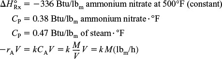
where M is the mass of ammonium nitrate in the CSTR (lbm) and k is given by the relationship below.

The enthalpies of water and steam are
Hw (200°F) = 168 Btu/lbm
Hg (500°F) = 1202 Btu/lbm
(a) Can you explain the cause of the blast? Hint: See Problem P13-3B.
(b) If the feed rate to the reactor just before shutoff was 310 lbm of solution per hour, what was the exact temperature in the reactor just prior to shutdown? Hint: Plot Qr and Qg as a function of temperature on the same plot.
(c) How would you start up or shut down and control such a reaction? (Hint: See Problem P13-2B.)
(d) Explore this problem and describe what you find. For example, add a heat exchanger UA (T – Ta), choose values of UA and Ta, and then plot R(T) versus G(T)?
(e) Discuss what you believe to be the point of the problem. The idea for this problem originated from an article by Ben Horowitz.
P12-6B The endothermic liquid-phase elementary reaction
A + B → 2C
proceeds, substantially, to completion in a single steam-jacketed, continuous-stirred reactor (Table P12-6B). From the following data, calculate the steady-state reactor temperature:
Reactor volume: 125 gal
Steam jacket area: 10 ft2

Jacket steam: 150 psig (365.9°F saturation temperature)
Overall heat-transfer coefficient of jacket, U: 150 Btu/h · ft2 · °F
Agitator shaft horsepower: 25 hp
Heat of reaction, ![]() = + 20,000
= + 20,000
Btu/lb-mol of A (independent of temperature)

P12-7B Use the data in Problem P11-4A for the following reaction.
Th elementary, irreversible, organic liquid-phase reaction
is carried out in a flow reactor. An equal molar feed in A and B enters at 27°C, and the volumetric flow rate is 2 dm3/s and CA0 = 0.1 kmol/m3.
Additional information:

(a) Calculate the conversion when the reaction is carried out adiabatically in one 500-dm3 CSTR and then compare the results with the two adiabatic 250-dm3 CSTRs in series.
The reversible reaction (part (d) of P11-4A) is now carried out in a PFR with a heat exchanger. Plot and then analyze X, Xe, T, Ta, Qr, Qg, and the rate, –rA, for the following cases:
(b) Constant heat-exchanger temperature Ta
(c) Co-current heat exchanger Ta (Ans.: At V = 10 m3 then X = 0.36 and T = 442 K)
(d) Countercurrent heat exchanger Ta (Ans.: At V = 10 m3 then X = 0.364 and T = 450 K)
(e) Adiabatic operation
(f) Make a table comparing all your results (e.g., X, Xe, T, Ta). Write a paragraph describing what you find.
(g) Plot Qr and Ta as a function of V necessary to maintain isothermal operation.
P12-8A The gas-phase reversible reaction as discussed in P11-7B
A ![]() B
B
is now carried out under high pressure in a packed-bed reactor with pressure drop. The feed consists of both inerts I and species A with the ratio of inerts to the species A being 2 to 1. The entering molar flow rate of A is 5 mol/min at a temperature of 300 K and a concentration of 2 mol/dm3. Work this problem in terms of volume. Hint: V = W/pB, ![]()
Additional information:
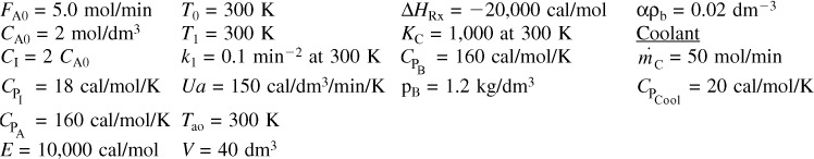
Plot and then analyze X, Xe, T, Ta, and the rate (–rA) profiles in a PFR for the following cases. In each case, explain why the curves look the way they do.
(a) Co-current heat exchange
(b) Countercurrent heat exchange (Ans.: When V = 20 dm3 then X = 0.86 and Xe = 0.94)
(c) Constant heat-exchanger temperature Ta
(d) Compare and contrast each of the above results and the results for adiabatic operation (e.g., make a plot or a table of X and Xe obtained in each case).
(e) Vary some of the parameters, e.g., (0 < ΘI < 10) and describe what you find.
(f) Plot Qr and Ta as a function of V necessary to maintain isothermal operation.
P12-9A Algorithm for reaction in a PBR with heat effects and pressure drop
The elementary gas-phase reaction
in P11-8B is now continued and carried out in packed-bed reactor. The entering molar flow rates are FA0 = 5 mol/s, FB0 = 2FA0, and FI = 2FA0 with CA0 = 0.2 mol/dm3. The entering temperature is 325 K and a coolant fluid is available at 300 K.
Additional information:
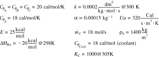
Plot X, Xe, T, Ta, and –rA down the length of the PFR for the following cases:
(a) Co-current heat exchange
(b) Countercurrent heat exchange
(c) Constant heat-exchanger temperature Ta
(d) Compare and contrast your results for (a), (b), and (c) along with those for adiabatic operation and write a paragraph describing what you find.
P12-10B Use the data and reaction in Problems P11-4A and P12-7A for the following:
(a) Plot and then analyze the conversion, Qr, Qg, and temperature profiles up to a PFR reactor volume of 10 dm3 for the case when the reaction is reversible with KC = 10 m3/kmol at 450 K. Plot and then analyze the equilibrium conversion profile.
(b) Repeat (a) when a heat exchanger is added, Ua = 20 cal/m3/s/K, and the coolant temperature is constant at Ta = 450 K.
(c) Repeat (b) for both a co-current and a countercurrent heat exchanger. The coolant flow rate is 50 g/s, CPc = 1 cal/g · K, and the inlet coolant temperature is Ta0 = 450 K. Vary the coolant rate (10 < ![]() < 1,000 g/s).
< 1,000 g/s).
(d) Plot Qr and Ta as a function of V necessary to maintain isothermal operation.
(e) Compare your answers to (a) through (d) and describe what you find. What generalizations can you make?
(f) Repeat (c) and (d) when the reaction is irreversible but endothermic with ![]() = 6,000 cal/mol. Choose Ta0 = 450 K.
= 6,000 cal/mol. Choose Ta0 = 450 K.
P12-11B Use the reaction data in Problem P11-4A and P12-7A for the case when heat is removed by a heat exchanger jacketing the reactor. The flow rate of coolant through the jacket is sufficiently high that the ambient exchanger temperature is constant at Ta = 50°C.
(a) (1) Plot and then analyze the temperature conversion, Qr, and Qg profiles for a PBR with
where
pb = bulk density of the catalyst (kg/m3)
a = heat-exchange area per unit volume of reactor (m2/m3)
U = overall heat-transfer coefficient (J/s · m2 · K)
(2) How would the profiles change if Ua/pb were increased by a factor of 3000?
(3) If there is a pressure drop with α = 0.019 kg–1?
(b) Repeat part (a) for co-current and countercurrent flow and adiabatic operation with ![]() = 0.2 kg/s, CPc = 5,000 J/kg K, and an entering coolant temperature of 50°C.
= 0.2 kg/s, CPc = 5,000 J/kg K, and an entering coolant temperature of 50°C.
(c) Find X and T for a “fluidized” CSTR with 80 kg of catalyst.
(d) Repeat parts (a) and (b) for W = 80.0 kg, assuming a reversible reaction with a reverse specific reaction rate of

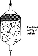
Vary the entering temperature, T0, and describe what you find.
(e) Use or modify the data in this problem to suggest another question or calculation. Explain why your question requires either critical thinking or creative thinking. See Preface Section I and http://www.umich.edu/scps.
P12-12C Derive the energy balance for a packed bed membrane reactor. Apply the balance to the reaction in Problem P11-5B
A ![]() B + C
B + C
for the case when it is reversible with KC = 1.0 mol/dm3 at 300 K. Species C diffuses out of the membrane with kC = 1.5 s–1.
(a) Plot and then analyze the concentration profiles for different values of KC when the reaction is carried out adiabatically.
(b) Repeat part (a) when the heat transfer coefficient is Ua = 30 J/s·kg-cat·K with Ta = 50°C.
P12-13B Circle the correct answer.
(a) The elementary reversible isomerization of A to B was carried out in a packed-bed reactor. The following profiles were obtained:
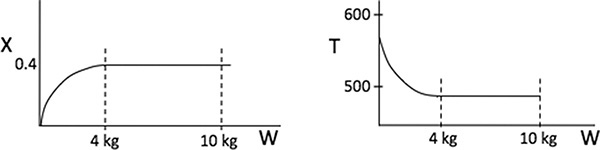
If the total entering volumetric flow rate remains constant, the addition of inerts to the feed stream will most likely
A) Increase conversion.
B) Decrease conversion.
C) Have no effect.
D) Insufficient information to tell
(b)
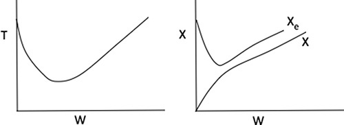
Which of the following statements are true?
A) The above reaction could be adiabatic.
B) The above reaction could be exothermic with constant cooling temperature.
C) The above reaction could be endothermic with constant heating temperature.
D) The above reaction could be second order.
P12-14A The irreversible reaction
is carried out adiabatically in a CSTR. The “heat generated” G(T) and the “heat removed” R(T) curves are shown in Figure P12-14A.
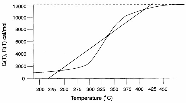
(a) What is the ΔHRx of the reaction?
(b) What are the inlet ignition and extinction temperatures?
(c) What are all the temperatures in the reactor corresponding to the inlet ignition and extinction temperatures?
(d) What are the conversions at the ignition and extinction temperatures?
P12-15B The first-order, irreversible, exothermic liquid-phase reaction
A → B
is to be carried out in a jacketed CSTR. Species A and an inert I are fed to the reactor in equimolar amounts. The molar feed rate of A is 80 mol/min.
Additional information

(a) What is the reactor temperature for a feed temperature of 450 K?
(b) Plot and then analyze the reactor temperature as a function of the feed temperature.
(c) To what inlet temperature must the fluid be preheated for the reactor to operate at a high conversion? What are the corresponding temperature and conversion of the fluid in the CSTR at this inlet temperature?
(d) Suppose that the fluid inlet temperature is now heated 5°C above the reactor temperature in part
(c) and then cooled 20°C, where it remains. What will be the conversion?
(e) What is the inlet extinction temperature for this reaction system? (Ans.: T0 = 87°C.)
P12-16B The elementary reversible liquid-phase reaction
takes place in a CSTR with a heat exchanger. Pure A enters the reactor.
(a) Derive an expression (or set of expressions) to calculate G (T) as a function of the heat of reaction, equilibrium constant, temperature, and so on. Show a sample calculation for G (T) at T = 400 K.
(b) What are the steady-state temperatures? (Ans.: 310, 377, 418 K.)
(c) Which steady states are locally stable?
(d) What is the conversion corresponding to the upper steady state?
(e) Vary the ambient temperature Ta and make a plot of the reactor temperature as a function of Ta, identifying the ignition and extinction temperatures.
(f) If the heat exchanger in the reactor suddenly fails (i.e., UA = 0), what would be the conversion and the reactor temperature when the new upper steady state is reached? (Ans.: 431 K.)
(g) What heat exchanger product, UA, will give the maximum conversion?
(h) Write a question that requires critical thinking and then explain why your question requires critical thinking. Hint: See Preface Section I.
(i) What is the adiabatic blowout flow rate, υ0 ?
(j) Suppose that you want to operate at the lower steady state. What parameter values would you suggest to prevent runaway, e.g., the upper SS?
Additional information
P12-17B The reversible liquid phase reaction
A ![]() B
B
is carried out in a 12-dm3 CSTR with heat exchange. Both the entering temperature, T0, and the heat exchange fluid, Ta, are at 330 K. An equal molar mixture of inerts and A enter the reactor.
(a) Choose a temperature, T, and carry out a calculation to find G(T) to show that your calculation agrees with the corresponding G(T) value on the curve shown below at the temperature you choose.
(b) Find the exit conversion and temperature from the CSTR. X = _______ T = _____.
(c) What entering temperature T0 would give you the maximum conversion? T0 = _______ X = ______
(d) What would the exit conversion and temperature be if the heat-exchange system failed (i.e., U = 0)?
(e) Can you find the inlet ignition and extinction temperatures? If yes, what are they? If not, go on to the next problem.
(f) Use Preface Section I to ask another question.
Additional information
The G(T) curve for this reaction is shown below
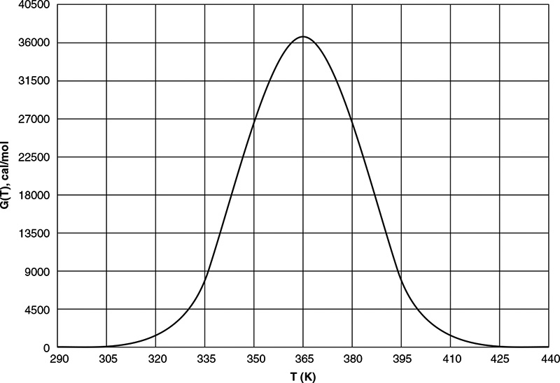
P12-18C The elementary gas-phase reaction
2A ![]() C
C
is carried out in a packed-bed reactor. Pure A enters the reactor at a 450-K flow rate of 10 mol/s, and a concentration of 0.25 mol/dm3. The PBR contains 90 kg of catalyst and is surrounded by a heat exchanger for which cooling fluid is available at 500 K. Compare the conversion achieved for the four types of heat exchanger operation: adiabatic, constant Ta, co-current flow, and countercurrent flow.
P12-19C A reaction is to be carried out in the packed-bed reactor shown in Figure P12-19C.
The reactants enter the annular space between an outer insulated tube and an inner tube containing the catalyst. No reaction takes place in the annular region. Heat transfer between the gas in this packed-bed reactor and the gas flowing countercurrently in the annular space occurs along the length of the reactor. The overall heat-transfer coefficient is 5 W/m2 · K. Plot the conversion and temperature as a function of reactor length for the data given in reactor length for the data given in Problem P12-7B
A + B ![]() 2C
2C
is carried out in a packed-bed reactor. Match the following temperature and conversion profiles for the four different heat-exchange cases: adiabatic, constant Ta, co-current exchange, and countercurrent exchange.
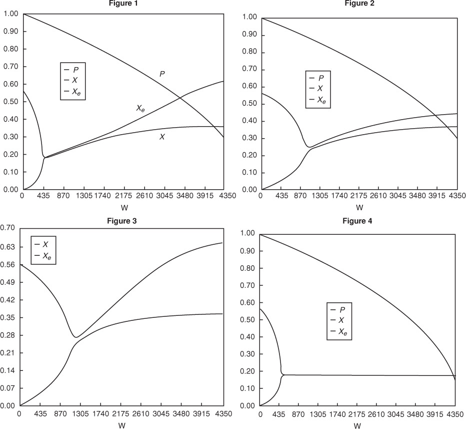
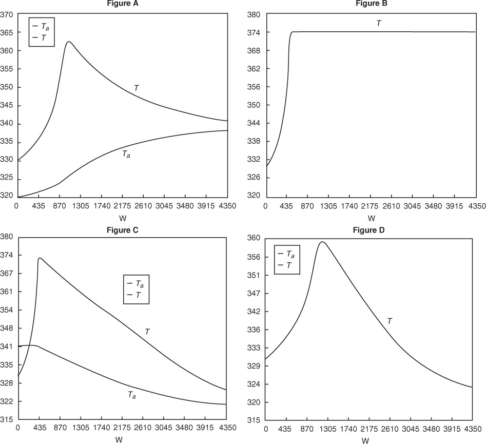
(a) Figure 1 matches Figure ________
(b) Figure 2 matches Figure ________
(c) Figure 3 matches Figure ________
(d) Figure 4 matches Figure ________
P12-21B The irreversible liquid-phase reactions
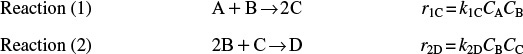
are carried out in a PFR with heat exchange. The following temperature profiles were obtained for the reactor and the coolant stream:
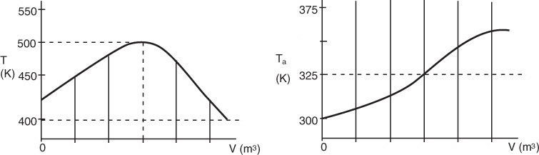
The concentrations of A, B, C, and D were measured at the point down the reactor where the liquid temperature, T, reached a maximum, and they were found to be CA = 0.1, CB = 0.2, CC = 0.5, and CD = 1.5, all in mol/dm3. The product of the overall heat-transfer coefficient and the heat-exchanger area per unit volume, Ua, is 10 cal/s · dm3 · K. The entering molar flow rate of A is 10 mol/s.
Additional information
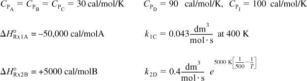
(a) What is the activation energy for Reaction (1)?
P12-22B The following elementary reactions are to be carried out in a PFR with a heat exchange with constant Ta:
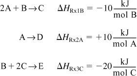
The reactants all enter at 400 K. Only A and B enter the reactor. The entering concentration of A and B are 3 molar and 1 molar at a volumetric flow rate of 10 dm3/s.
Additional information
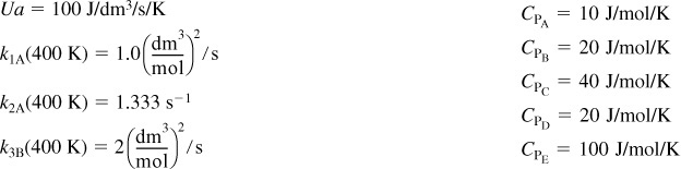
What constant coolant temperature, Ta, is necessary such that at the reactor entrance, i.e., V = 0, ![]() ?
?
P12-23B The complex gas-phase reactions are elementary
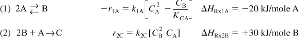
and carried out in a PFR with a heat exchanger. Pure A enters at a rate of 5 mol/min, a concentration of 0.2 mol/dm3, and temperature 300 K. The entering temperature of an available coolant is 320 K.
k1A1 = 50 dm3/mol • min@305 K with E1 = 8,000 J/mol
k2C2 = 4000 dm9/mol3 • min@310 K with E2 = 4,000 J/mol
KCA = 10 dm3/mol@315 K
Note: This is the equilibrium constant with respect to A in reaction 1 when
using van Hoff’s equation, i.e., (S12-4),
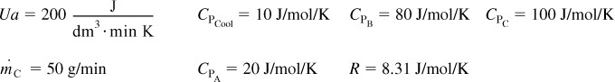
The reactor volume is 10 dm3.
(a) Plot (FA, FB, FC) on one graph and (T and Ta) on another along the length of the reactor for adiabatic operation, heat exchange with constant Ta, and co-current and countercurrent heat exchange with variable Ta. Only turn in a copy of your code and output for co-current exchange.
Adiabatic operation
(b) What is the maximum temperature and at what reactor volume is it reached?
(c) At what reactor volume is the flow rate of B a maximum, and what is FBmax at this value?
Constant Ta
(d) What is the maximum temperature and at what reactor volume is it reached?
(e) At which reactor volume is the flow rate of B a maximum, and what is FBmax at this volume?
Co-current exchange
(f) At what reactor volume does Ta become greater than T? Why does it become greater
Countercurrent exchange
(g) At what reactor volume does Ta become greater than T?
Hint: Guess Ta at entrance around 350 K.
P12-24B The elementary liquid-phase reactions
are carried out adiabatically in a 10 dm3 PFR. After streams A and B mix, species A enters the reactor at a concentration of CA0 = 2 mol/dm3 and species B at a concentration of 4 mol/dm3. The entering volumetric flow rate is 10 dm3/s.
Assuming you could vary the entering temperature between 300 K and 600 K, what entering temperture would you recommend to maximize the concentration of species C exiting the reactor? (±25˚K). Assume all species have the same density.
Additional information
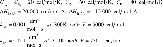
P12-25C (Multiple reactions with heat effects) Xylene has three major isomers, m-xylene (A), o-xylene (B), and p-xylene (C). When m-xylene (A) is passed over a Cryotite catalyst, the following elementary reactions are observed. The reaction to form p-xylene is irreversible:
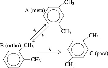
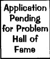
The feed to the reactor is pure m-xylene (A). For a total feed rate of 2 mol/min and the reaction conditions below, plot the temperature and the molar flow rates of each species as a function of catalyst weight up to a weight of 100 kg.
(a) Plot the concentrations of each of xylenes down the length (i.e., V) of a PBR.
(b) Find the lowest concentration of o-xylene achieved in the reactor.
(c) Find the maximum concentration of o-xylene in the reactor.
(d) Repeat part (a) for a pure feed of o-xylene (B). What is the maximum concentration of meta xylene and where does it occur in the reactor?
(e) Vary some of the system parameters and describe what you learn.
(f) What do you believe to be the point of this problem?
Additional information9
9 Obtained from inviscid pericosity measurements.
All heat capacities are virtually the same at 100 J/mol ·K.
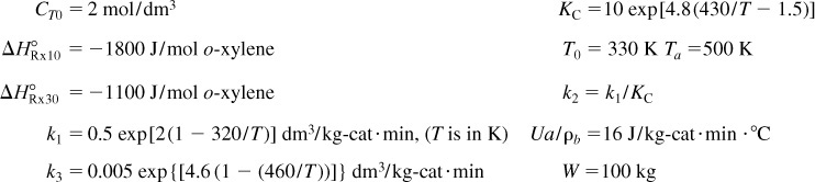
P12-26C (Comprehensive problem on multiple reactions with heat effects) Styrene can be produced from ethylbenzene by the following reaction:
However, several irreversible side reactions also occur:
[J. Snyder and B. Subramaniam, Chem. Eng. Sci., 49, 5585 (1994)]. Ethylbenzene is fed at a rate of 0.00344 kmol/s to a 10.0-m3 PFR (PBR), along with inert steam at a total pressure of 2.4 atm. The steam/ethylbenzene molar ratio is initially, i.e., parts (a) to (c), 14.5 : 1 but can be varied.
Given the following data, find the exiting molar flow rates of styrene, benzene, and toluene along with ![]() for the following inlet temperatures when the reactor is operated adiabatically:
for the following inlet temperatures when the reactor is operated adiabatically:
(a) T0 = 800 K
(b) T0 = 930 K
(c) T0 = 1100 K
(d) Find the ideal inlet temperature for the production of styrene for a steam/ethylbenzene ratio of 58 : 1. Hint: Plot the molar flow rate of styrene versus T0 . Explain why your curve looks the way it does.
(e) Find the ideal steam/ethylbenzene ratio for the production of styrene at 900 K. Hint: See part (d).
(f) It is proposed to add a countercurrent heat exchanger with Ua = 100 kJ/m3/min/K, where Ta is virtually constant at 1000 K. For an entering stream to ethylbenzene ratio of 20, what would you suggest as an entering temperature? Plot the molar flow rates and ![]() .
.
(g) What do you believe to be the major points of this problem?
(h) Ask another question or suggest another calculation that can be made for this problem.
Additional information

The kinetic rate laws for the formation of styrene (St), benzene (B), and toluene (T), respectively, are as follows (EB = ethylbenzene).

The temperature T is in Kelvin and Pi is in atm.
P12-27B The liquid-phase, dimer-quadmer series addition reaction
4A → 2A2 → A4
can be written as

and is carried out in a 10-dm3 PFR. The mass flow rate through the heat exchanger surrounding the reactor is sufficiently large so that the ambient temperature of the exchanger is constant at Ta = 315 K. The reactants enter at a temperature T0, of 300 K. Pure A is fed to the rector at a volumetric flow rate of 50 dm3/s and a concentration of 2 mol/dm3.
(a) Plot, compare, and analyze the profiles FA, FA2, and FA4 down the length of the reactor up to 10 dm3.
(b) The desired product is A2 and it has been suggested that the current reactor may be too large. What reactor volume would you recommend to maximize FA2?
(c) What operating variables (e.g., T0, Ta) would you change and how would you change them to make the reactor volume as small as possible and to still maximize FA2? Note any opposing factors in maximum production of A2. The ambient temperature and the inlet temperature must be kept between 0˚C and 177˚C.
Additional information
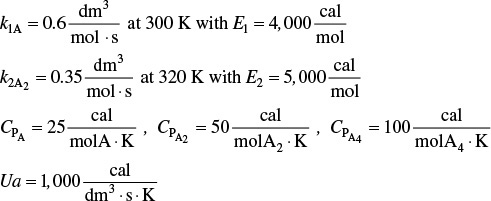
Turn in your recommendation of reactor volume to maximize FA2 and the molar flow rate at this maximum.
Supplementary Reading
1. An excellent development of the energy balance is presented in
ARIS, R., Elementary Chemical Reactor Analysis. Upper Saddle River, NJ: Prentice Hall, 1969, Chaps. 3 and 6.
FOGLER, JOSEPH, A Reaction Engineer’s Handbook of Thermochemical Data, Jofostan Press, Riça, Jofostan (2018).
CENTER FOR CHEMICAL PROCESS SAFETY (CCPS), Guidelines for Chemical Reactivity Evaluation and Application to Process Design. New York: American Institute of Chemical Engineers (AIChE) 1995.
CROWL, DANIEL A., and JOSEPH F. LOUVAR, Chemical Process Safety: Fundamentals with Applications, 3rd ed. Upper Saddle River, NJ: Prentice Hall, 2011.
MELHEM, G. A., and H. G. FISHER, International Symposium on Runaway Reactions and Pressure Relief Design. New York: Center for Chemical Process Safety (CCPS) of the American Institute of Chemical Engineers (AIChE) and The Institution of Chemical Engineers, 1995.
See the Center for Chemical Process Safety (CCPS) Web site, www.aiche.org/ccps.
3. A number of example problems dealing with nonisothermal reactors may or may not be found in
BURGESS, THORNTON W., The Adventures of Jerry Muskrat. New York: Dover Publications, Inc., 1914.
FROMENT, G. F., and K. B. BISCHOFF, Chemical Reactor Analysis and Design, 3rd ed. New York: Wiley, 2010.
WALAS, S. M., Chemical Reaction Engineering Handbook of Solved Problems. Amsterdam: Gordon and Breach, 1995. See the following solved problems: Problem 4.10.1, page 444; Problem 4.10.08, page 450; Problem 4.10.09, page 451; Problem 4.10.13, page 454; Problem 4.11.02, page 456; Problem 4.11.09, page 462; Problem 4.11.03, page 459; Problem 4.10.11, page 463.
4. A review of the multiplicity of the steady state and reactor stability is discussed by
PERLMUTTER, D. D., Stability of Chemical Reactors. Upper Saddle River, NJ: Prentice Hall, 1972.
5. The heats of formation, Hi (T), Gibbs free energies, Gi (TR), and the heat capacities of various compounds can be found in
GREEN, DON W., and ROBERT H. PERRY, Perry’s Chemical Engineers’ Handbook, 8th ed. (Chemical Engineers Handbook). New York: McGraw-Hill, 2008.
LIDE DAVID R., CRC Handbook of Chemistry and Physics, 90th ed. Boca Raton, FL: CRC Press, 2009.