14. Mass Transfer Limitations in Reacting Systems
Giving up is the ultimate tragedy.
—Robert J. Donovan
or
It ain’t over ’til it’s over.
—Yogi Berra NY Yankees
14.1 Diffusion Fundamentals
The first step in our CRE algorithm is the mole balance, which we now need to extend to include the molar flux, WAz, and diffusional effects. The molar flow rate of A in a given direction, such as the z direction down the length of a tubular reactor, is just the product of the flux, WAz (mol/m2 • s), and the cross-sectional area, Ac (m2); that is,
FAz = Ac WAz
The Algorithm
1. Mole balance
2. Rate law
3. Stoichiometry
4. Combine
5. Evaluate
In the previous chapters, we have only considered plug flow with no diffusion superimposed, in which case
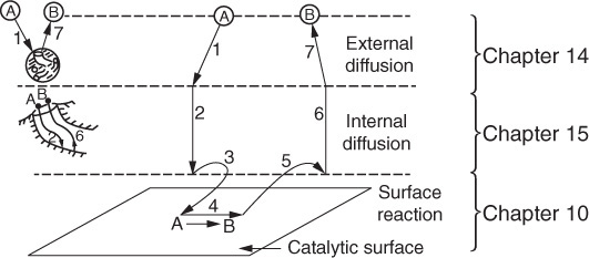
We now drop the plug-flow assumption and extend our discussion of mass transfer in catalytic and other mass-transfer limited reactions. In Chapter 10 we focused on the middle three steps (3, 4, and 5) in a catalytic reaction and neglected steps (1), (2), (6), and (7) by assuming the reaction was surface-reaction limited. In this chapter we describe the first and last steps (1) and (7), as well as showing other applications in which mass transfer plays a role.
Where are we going ??:†
† “If you don’t know where you are going, you’ll probably wind up some place else.” Yogi Berra, NY Yankees
We want to arrive at the mole balance that incorporates both diffusion and reaction effects, such as Equation (14-16) on page 685. I.e.,

We begin with Section 14.1.1 where we write the mole balance on Species A in three dimensions in terms of the molar flux, WA. In Section 14.1.2 we write WA in terms of the bulk flow of A in the fluid, BA and the diffusion flux JA of A that is superimposed on bulk flow. In Section 14.1.3 we use the previous two subsections as a basis to finally write the molar flux, WA, in terms of concentration using Fick’s first law, JA, and the bulk flow, BA. Next, in Section 14.2 we combine diffusion convective transport and reaction in our mole balance.
14.1.1 Definitions
Diffusion is the spontaneous intermingling or mixing of atoms or molecules by random thermal motion. It gives rise to motion of the species relative to motion of the mixture. In the absence of other gradients (such as temperature, electric potential, or gravitational potential), molecules of a given species within a single phase will always diffuse from regions of higher concentrations to regions of lower concentrations. This gradient results in a molar flux of the species (e.g., A), WA (moles/area ·time), in the direction of the concentration gradient. The flux of A, WA, is relative to a fixed coordinate (e.g., the lab bench) and is a vector quantity with typical units of mol/m2 · s. In rectangular coordinates
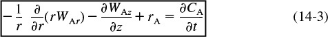
We now apply the mole balance to species A, which flows and reacts in an element of volume ΔV = ΔxΔyΔz to obtain the variation of the molar fluxes in three dimensions.


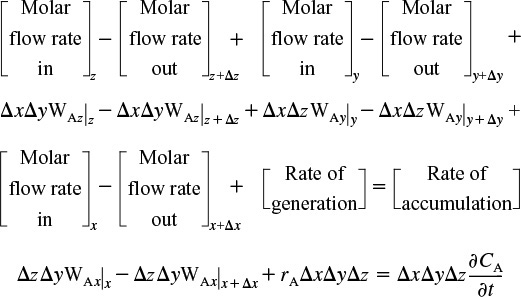
Mole Balance
where rA is the rate of generation of A by reaction per unit volume (e.g., mol/m3/h).
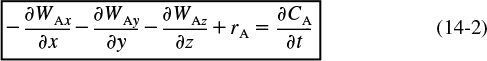
Dividing by ΔxΔyΔz and taking the limit as they go to zero, we obtain the molar flux balance in rectangular coordinates
The corresponding balance in cylindrical coordinates with no variation in the rotation about the z-axis is
COMSOL
We will now evaluate the flux terms WA. We have taken the time to derive the molar flux equations in this form because they are now in a form that is consistent with the partial differential equation (PDE) solver COMSOL, which is accessible from the CRE Web site.
14.1.2 Molar Flux
The molar flux of A, WA, is the result of two contributions: JA, the molecular diffusion flux relative to the bulk motion of the fluid produced by a concentration gradient, and BA, the flux resulting from the bulk motion of the fluid:
Total flux = diffusion + bulk motion
The bulk-flow term for species A is the total flux of all molecules relative to a fixed coordinate times the mole fraction of A, yA; i.e., BA = yA ∑ Wi.
For a two-component system of A diffusing in B, the flux of A is
The diffusional flux, JA, is the flux of A molecules that is superimposed on the bulk flow. It tells how fast A is moving ahead of the bulk flow velocity, i.e., the molar average velocity.
The flux of species A, WA, is wrt a fixed coordinate system (e.g., the lab bench) and is just the concentration of A, CA, times the particle velocity of species A, UA, at that point
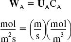
By particle velocities, we mean the vector average of millions of molecules of A at a given point. Similarity for species B: WB = UBCB; substituting into the bulk-flow term
BA = yA ∑ Wi = yA (WA + WB) = yA (CA UA + CBUB)
Writing the concentration of A and B in the generic form in terms of the mole fraction, yi, and the total concentration, c, i.e., Ci = yic, and then factoring out the total concentration, c, the bulk flow, BA, is
BA = (c yA)(yA UA + yBUB) = CA U
Molar average velocity
where U is the molar average velocity: U = ∑ yi Ui. The molar flux of A can now be written as
We now need to determine the equation for the molar flux of A, JA, that is superimposed on the molar average velocity.
14.1.3 Fick’s First Law
Our discussion on diffusion will be restricted primarily to binary systems containing only species A and B. We now wish to determine how the molar diffusive flux of a species (i.e., JA) is related to its concentration gradient. As an aid in the discussion of the transport law that is ordinarily used to describe diffusion, recall similar laws from other transport processes. For example, in conductive heat transfer the constitutive equation relating the heat flux q and the temperature gradient is Fourier’s law, q = –kt ∇T, where kt is the thermal conductivity.
Experimentation with frog legs led to Fick’s first law.
In rectangular coordinates, the gradient is in the form
Constitutive equations in heat, momentum, and mass transfer
The mass transfer law for the diffusional flux of A resulting from a concentration gradient is analogous to Fourier’s law for heat transfer and is given by Fick’s first law
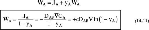
DAB is the diffusivity of A in B ![]() . Combining Equations (14-7) and (14-6), we obtain an expression for the molar flux of A in terms of concentration for constant total concentration
. Combining Equations (14-7) and (14-6), we obtain an expression for the molar flux of A in terms of concentration for constant total concentration
Molar flux equation
In one dimension, i.e., z, the molar flux term is
14.2 Binary Diffusion
Although many systems involve more than two components, the diffusion of each species can be treated as if it were diffusing through another single species rather than through a mixture by defining an effective diffusivity.
14.2.1 Evaluating the Molar Flux
We now consider five typical cases in Table 14-1 of A diffusing in B. Substituting Equation (14-7) into Equation (14-6) we obtain
Now the task is to evaluate the bulk-flow term.
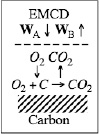
(1) Equal molar counter diffusion (EMCD) of species A and B. For every molecule of A that diffuses in the forward direction, one molecule of B diffuses in the reverse direction
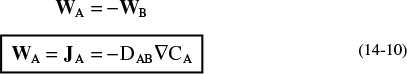
An example of EMCD is the oxidation of solid carbon; for every mole of oxygen that diffuses to the surface to react with the carbon surface, one mole of carbon dioxide diffuses away from the surface. WO2 = –WCO2
(2) Species A diffusing through stagnant species B (WB = 0). This situation usually occurs when a solid boundary is involved and there is a stagnant fluid layer next to the boundary through which A is diffusing
(3) Bulk flow of A is much greater than molecular diffusion of A, i.e., BA >> JA
This case is the plug-flow model we have been using in the previous chapters in this book
(4) For small bulk flow JA >> BA, we get the same result as EMCD, i.e., Equation (14-10)
(5) Knudsen Diffusion: Occurs in porous catalysts where the diffusing molecules collide more often with the pore walls than with each other
and DK is the Knudsen diffusion.1
1 C. N. Satterfield, Mass Transfer in Heterogeneous Catalysis (Cambridge: MIT Press, 1970), pp. 41–42, discusses Knudsen flow in catalysis and gives the expression for calculating DK .
TABLE 14-1 EVALUATING WA FOR SPECIES A DIFFUSING IN SPECIES B
14.2.2 Diffusion and Convective Transport
When accounting for diffusional effects, the molar flow rate of species A, FA, in a specific direction z, is the product of molar flux in that direction, WAz, and the cross-sectional area normal to the direction of flow, Ac
FAz = AcWAz
In terms of concentration, the flux is
The molar flow rate is
Similar expressions follow for WAx and WAy. Substituting for the flux WAx, WAy, and WAz into Equation (14-2), we obtain
Flow, diffusion, and reaction

This form is used in COMSOL Multiphysics.
Equation (14-15) is in a user-friendly form to apply to the PDE solver, COMSOL. For one dimension at steady state, Equation (14-15) reduces to
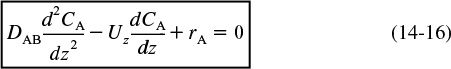
In order to solve Equation (14-16) we need to specify the boundary conditions. In this chapter we will consider some of the simple boundary conditions, and in Chapter 18 we will consider the more complicated boundary conditions, such as the Danckwerts’ boundary conditions.
We will now use this form of the molar flow rate in our mole balance in the z direction of a tubular flow reactor
However, we first have to discuss the boundary conditions in solving this equation.
14.2.3 Boundary Conditions
The most common boundary conditions are presented in Table 14-2.
1. Specify a concentration at a boundary (e.g., z = 0, CA = CA0).
For an instantaneous reaction at a boundary, the concentration of the reactants at the boundary is taken to be zero (e.g., CAs = 0). See Chapter 18 for the more exact and complicated Danckwerts’ boundary conditions at z = 0 and z = L.
2. Specify a flux at a boundary.
a. No mass transfer to a boundary
for example, at the wall of a nonreacting pipe. Species A cannot diffuse into the solid pipe wall so WA = 0 and then
That is, because the diffusivity is finite, the only way the flux can be zero is if the concentration gradient is zero.
b. Set the molar flux to the surface equal to the rate of reaction on the surface
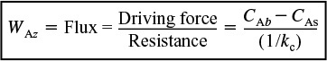
c. Set the molar flux to the boundary equal to convective transport across a boundary layer
where kc is the mass transfer coefficient and CAs and CAb are the surface and bulk concentrations, respectively.
3. Planes of symmetry. When the concentration profile is symmetrical about a plane, the concentration gradient is zero in that plane of symmetry. For example, in the case of radial diffusion in a pipe, at the center of the pipe
TABLE 14-2 TYPES OF BOUNDARY CONDITIONS
14.2.4 Temperature and Pressure Dependence of DAB
Before closing this brief discussion on mass-transfer fundamentals, further mention should be made of the diffusion coefficient.2 Equations for predicting gas diffusivities are given by Fuller and are also given in Perry’s Handbook.3,4 The orders of magnitude of the diffusivities for gases, liquids, and solids and the manner in which they vary with temperature and pressure are given in Table 14-3.5 We note that the Knudsen, liquid, and solid diffusivities are independent of total pressure.
2 For further discussion of mass-transfer fundamentals, see R. B. Bird, W. E. Stewart, and E. N. Lightfoot, Transport Phenomena, 2nd ed. (New York: Wiley, 2002).
3 E. N. Fuller, P. D. Schettler, and J. C. Giddings, Ind. Eng. Chem., 58(5), 19 (1966). Several other equations for predicting diffusion coefficients can be found in B. E. Polling, J. M. Prausnitz, and J. P. O’Connell, The Properties of Gases and Liquids, 5th ed. (New York: McGraw-Hill, 2001).
4 R. H. Perry and D. W. Green, Chemical Engineer’s Handbook, 7th ed. (New York: McGraw-Hill, 1999).
5 To estimate liquid diffusivities for binary systems, see K. A. Reddy and L. K. Doraiswamy, Ind. Eng. Chem. Fund., 6, 77 (1967).
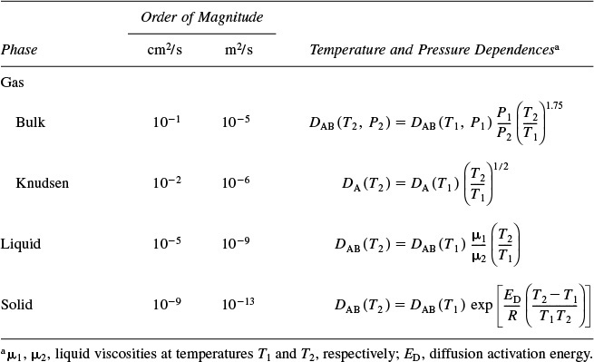
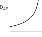
It is important to know the magnitude and the T and P dependence of the diffusivity.
Gas:

Liquid:
14.2.5 Steps in Modeling Diffusion to a Reacting Surface
We first consider the diffusion of species A through a stagnant film in which no reaction takes place to a catalytic surface where Species A reacts instantaneously by upon reaching the surface, i.e., CAs ≅ 0. Consequently, the rate of diffusion through the stagnant film equals the rate of reaction on the surface. The first steps in modeling are:
Step 1: Perform a differential mole balance on a particular species A or use the general mole balance, to obtain an equation for WAz, e.g., Equation (14-2).
Step 2: Replace WAz by the appropriate expression for the concentration gradient.
Step 3: State the boundary conditions.
Step 4: Solve for the concentration profile.
Step 5: Solve for the molar flux.
Steps in modeling mass transfer
In Section 14.3, we are going to apply this algorithm to one of the most important cases, diffusion through a boundary layer. Here, we consider the boundary layer to be a hypothetical “stagnant film” in which all the resistance to mass transfer is lumped.
14.2.6 Modeling Diffusion with Chemical Reaction
Next, we consider the situation where species A reacts as it diffuses through the stagnant film.6 This table will provide the foundation for problems with diffusion and reaction in both Chapters 14 and 15.
6 E. L. Cussler, Diffusion Mass Transfer in Fluid Systems, 2nd ed. (New York: Cambridge University Press, 1997).
Use Table 14-4 to In ![]() Out of the algorithm (Steps 1 → 6) to generate creative solutions.
Out of the algorithm (Steps 1 → 6) to generate creative solutions.
The purpose of presenting algorithms (e.g., Table 14-4) to solve reaction engineering problems is to give the readers a starting point or framework with which to work if they were to get stuck. It is expected that once readers are familiar and comfortable using the algorithm/framework, they will be able to move in and out of the framework as they develop creative solutions to nonstandard chemical reaction engineering problems.

Expanding the previous six modeling steps just a bit
1. Define the problem and state the assumptions.
2. Define the system on which the balances are to be made.
3. Perform a differential mole balance on a particular species.
4. Obtain a differential equation in WA by rearranging your balance equation properly and taking the limit as the volume of the element goes to zero.
5. Substitute the appropriate expression involving the concentration gradient for WA from Section 14.2 to obtain a second-order differential equation for the concentration of A.a
a In some instances it may be easier to integrate the resulting differential equation in Step 4 before substituting for WA.
6. Express the reaction rate rA (if any) in terms of concentration and substitute into the differential equation.
7. State the appropriate boundary and initial conditions.
8. Put the differential equations and boundary conditions in dimensionless form.
9. Solve the resulting differential equation for the concentration profile.
10. Differentiate this concentration profile to obtain an expression for the molar flux of A.
11. Substitute numerical values for symbols.
TABLE 14-4 STEPS IN MODELING CHEMICAL SYSTEMS WITH DIFFUSION AND REACTION
14.3 Diffusion Through a Stagnant Film
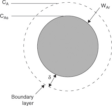
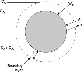
To begin our discussion on the diffusion of reactants from the bulk fluid to the external surface of a catalyst, we shall focus attention on the flow past a single catalyst pellet. Reaction takes place only on the external catalyst surface and not in the fluid surrounding it. The fluid velocity in the vicinity of the spherical pellet will vary with position around the sphere. The hydrodynamic boundary layer is usually defined as the distance from a solid object to where the fluid velocity is 99% of the bulk velocity, U0 . Similarly, the mass transfer boundary-layer thickness, δ, is defined as the distance from a solid object to where the concentration of the diffusing species reaches 99% of the bulk concentration.
A reasonable representation of the concentration profile for a reactant A diffusing to the external surface is shown in Figure 14-2. As illustrated, the change in concentration of A from CAb to CAs takes place in a very narrow fluid layer next to the surface of the sphere. Nearly all of the resistance to mass transfer is found in this layer.

The concept of a hypothetical stagnant film within which all the resistance to external mass transfer exists
A useful way of modeling diffusive transport is to treat the fluid layer next to a solid boundary as a hypothetical stagnant film of thickness δ, which we cannot measure. We say that all the resistance to mass transfer is found (i.e., lumped) within this hypothetical stagnant film of thickness δ, and the properties (i.e., concentration, temperature) of the fluid at the outer edge of the film are identical to those of the bulk fluid. This model can readily be used to solve the differential equation for diffusion through a stagnant film. The dashed line in Figure 14-2b represents the concentration profile predicted by the hypothetical stagnant film model, while the solid line gives the actual profile. If the film thickness is much smaller than the radius of the pellet (which is usually the case), curvature effects can be neglected. As a result, only the one-dimensional diffusion equation must be solved, as was shown in Figure 14-3.
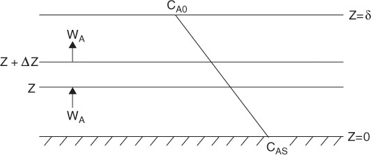
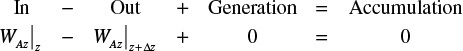
We are going to carry out a mole balance on species A diffusing through the fluid between z = z and z = z + Δz at steady state for the unit cross-sectional area, Ac
dividing by Δz and taking the limit as Δz → 0
For diffusion through a stagnant film at dilute concentrations
or for EMCD, we have using Fick’s first law
Substituting for WAz and dividing by DAB we have
Integrating twice to get CA = K1z + K2, using the boundary conditions at
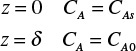
we obtain the concentration profile
To find the flux to the surface we substitute Equation (14-25) into Equation (14-24) to obtain
At steady state the flux of A to the surface will be equal to the rate of reaction of A on the surface. We also note that another example of diffusion through a stagnant film as applied to transdermal drug delivery is given in the Chapter 14 Expanded Material on the CRE Web site.
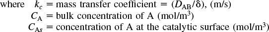
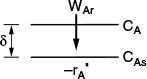
14.4 The Mass Transfer Coefficient
We now interpret the ratio (DAB/δ) in Equation (14-26).
While the boundary-layer thickness will vary around the sphere, we will take it to have a mean film thickness δ. The ratio of the diffusivity DAB to the film thickness δ is the mass transfer coefficient, kc, that is,

The mass transfer coefficient
Combining Equations (14-26) and (14-27), we obtain the average molar flux from the bulk fluid to the surface
Molar flux of A to the surface
In this stagnant film model, we consider all the resistance to mass transfer to be lumped into the thickness δ. The reciprocal of the mass transfer coefficient can be thought of as this resistance
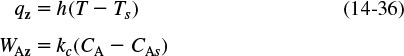
14.4.1 Correlations for the Mass Transfer Coefficient
The mass transfer coefficient kc is analogous to the heat transfer coefficient h. The heat flux q from the bulk fluid at a temperature T0 to a solid surface at Ts is
For forced convection, the heat transfer coefficient is normally correlated in terms of three dimensionless groups: the Nusselt number, Nu; the Reynolds number, Re; and the Prandtl number, Pr. For the single spherical pellets discussed here, Nu and Re take the following forms
The Prandtl number is not dependent on the geometry of the system


The Nusselt, Prandtl, and Reynolds numbers are used in forced convection heat transfer correlations.
The other symbols are as defined previously.
The heat transfer correlation relating the Nusselt number to the Prandtl and Reynolds numbers for flow around a sphere is7
7 W. E. Ranz and W. R. Marshall, Jr., Chem. Eng. Prog., 48, 141–146, 173–180 (1952).
Although this correlation can be used over a wide range of Reynolds numbers, it can be shown theoretically that if a sphere is immersed in a stagnant fluid (Re = 0), then
and that at higher Reynolds numbers in which the boundary layer remains laminar, we can neglect the 2 in Equation (14-34), in which case he Nusselt number becomes
Converting a heat transfer correlation to a mass transfer correlation
Although further discussion of heat transfer correlations is no doubt worthwhile, it will not help us to determine the mass transfer coefficient and the mass flux from the bulk fluid to the external pellet surface. However, the preceding discussion on heat transfer was not entirely futile because, for similar geometries, the heat and mass transfer correlations are analogous. If a heat transfer correlation for the Nusselt number exists, the mass transfer coefficient can be estimated by replacing the Nusselt and Prandtl numbers in this correlation by the Sherwood and Schmidt numbers, respectively:
The heat and mass transfer coefficients are analogous.† The corresponding fluxes are
† Strictly speaking, replacing the Nusselt number by the Sherwood number is only valid for situations where the Lewis number, Le, is close to 1. ![]()
The one-dimensional differential forms of the mass flux for EMCD and the heat flux are, respectively,
For EMCD the heat and molar flux equations are analogous.
If we replace h by kc and kt by DAB in Equation (14-30), i.e.,
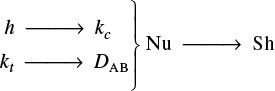
we obtain the mass transfer Nusselt number (i.e., the Sherwood number)
Sherwood number
The Prandtl number is the ratio of the kinematic viscosity (i.e., the momentum diffusivity) to the thermal diffusivity. Because the Schmidt number is analogous to the Prandtl number, one would expect that Sc is the ratio of the momentum diffusivity (i.e., the kinematic viscosity), υ, to the mass diffusivity DAB. Indeed, this is true
The Schmidt number is
Schmidt number
Consequently, the correlation for mass transfer for flow around a spherical pellet is analogous to that given for heat transfer, Equation (14-33); that is,
This relationship is often referred to as the Frössling correlation.8
8 N. Frössling, Gerlands Beitr. Geophys., 52, 170 (1938).
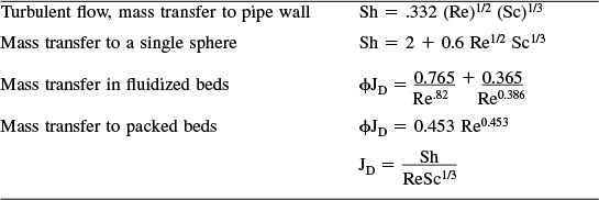
A few additional correlations for the Sherwood number from which one can determine the mass transfer coefficient are given in Table 14-5.
The Sherwood, Reynolds, and Schmidt numbers are used in forced convection mass transfer correlations.
14.4.2 Mass Transfer to a Single Particle
In this section we consider two limiting cases of diffusion and reaction on a catalyst particle.9 In the first case, the reaction is so rapid that the rate of diffusion of the reactant to the surface limits the reaction rate. In the second case, the reaction is so slow that virtually no concentration gradient exists in the gas phase (i.e., rapid diffusion with respect to surface reaction).
9 A comprehensive list of correlations for mass transfer to particles is given by G. A. Hughmark, Ind. Eng. Chem. Fund., 19(2), 198 (1980).
Example 14–1 Rapid Reaction on the Surface of a Catalyst
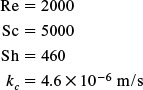
Calculate the molar flux, WAr, of reactant A to a single catalyst pellet 1 cm in diameter suspended in a large body of liquid B. The reactant is present in dilute concentrations, and the reaction is considered to take place instantaneously at the external pellet surface (i.e., CAs ![]() 0). The bulk concentration of the reactant A is 1.0 M, and the free-stream liquid velocity past the sphere is 0.1 m/s. The kinematic viscosity (i.e.,
0). The bulk concentration of the reactant A is 1.0 M, and the free-stream liquid velocity past the sphere is 0.1 m/s. The kinematic viscosity (i.e., ![]() ) is 0.5 centistoke (cS; 1 centistoke = 10–6 m2/s), and the liquid diffusivity of A in B is DAB = 10–10 m2/s, at 300 K.
) is 0.5 centistoke (cS; 1 centistoke = 10–6 m2/s), and the liquid diffusivity of A in B is DAB = 10–10 m2/s, at 300 K.
If the surface reaction is rapid, then diffusion limits the overall rate.
For dilute concentrations of the solute, the radial flux is
Because reaction is assumed to occur instantaneously on the external surface of the pellet, CAs = 0. Also, CAb is given as 1 mol/dm3. The mass transfer coefficient for single spheres is calculated from the Frössling correlation

Liquid Phase
Substituting these values into Equation (14-40) gives us
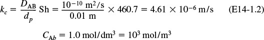
Substituting for kc and CAb in Equation (14-26), the molar flux to the surface is
WAr = (4.61 × 10⁻⁶) m/s (103 – 0) mol/m3 = 4.61 × 10⁻³ mol/m2 · s
Because ![]() , this rate is also the rate of reaction per unit surface area of catalyst.
, this rate is also the rate of reaction per unit surface area of catalyst.
Analysis: In this example we calculated the rate of reaction on the external surface of a catalyst pellet when external mass transfer was limiting the reaction rate. To determine the rate of reaction, we used correlations to calculate the mass transfer coefficient and then used kc to calculate the flux to the surface, which in turn was equal to the rate of surface reaction.
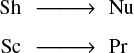
In Example 14-1, the surface reaction was extremely rapid and the rate of mass transfer to the surface dictated the overall rate of reaction. We now consider a more general case. The isomerization
is taking place on the surface of a solid sphere (Figure 14-4). The surface reaction follows a Langmuir–Hinshelwood single-site mechanism for which the rate law is

The temperature is sufficiently high that we only need to consider the case of very weak adsorption (i.e., low surface coverage) of A and B; thus
Therefore, the rate law becomes apparent first order
Using boundary conditions 2b and 2c in Table 14-1, we obtain
The concentration CAs is not as easily measured as the bulk concentration. Consequently, we need to eliminate CAs from the equation for the flux and rate of reaction. Solving Equation (14-44) for CAs yields
and the rate of reaction on the surface becomes
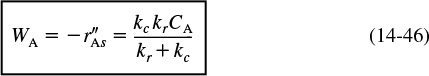
Molar flux of A to the surface is equal to the rate of consumption of A on the surface.
One will often find the flux to or from the surface written in terms of an effective transport coefficient keff
where
Rapid Reaction. We first consider how the overall rate of reaction may be increased when the rate of mass transfer to the surface limits the overall rate of reaction. Under these circumstances, the specific reaction rate constant is much greater than the mass transfer coefficient
and
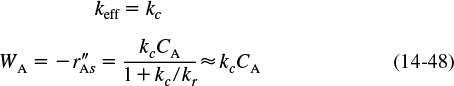
To increase the rate of reaction per unit surface area of a solid sphere, one must increase CA and/or kc . In this gas-phase catalytic reaction example, and for most liquids, the Schmidt number is sufficiently large that the number 2 in Equation (14-40) is negligible with respect to the second term when the Reynolds number is greater than 25. As a result, Equation (14-40) gives
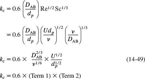
It is important to know how the mass transfer coefficient varies with fluid velocity, particle size, and physical properties.
Term 1 is a function of the physical properties DAB and υ, which depend on temperature and pressure only. The diffusivity always increases with increasing temperature for both gas and liquid systems. However, the kinematic viscosity υ increases with temperature (υ ∝ T3/2) for gases and decreases exponentially with temperature for liquids. Term 2 is a function of flow conditions and particle size. Consequently, to increase kc and thus the overall rate of reaction per unit surface area, one may either decrease the particle size or increase the velocity of the fluid flowing past the particle. For this particular case of flow past a single sphere, we see that if the velocity is doubled, the mass transfer coefficient and consequently the rate of reaction is increased by a factor of
(U2/U1)0.5 = 20.5 = 1.41 or 41%
Mass Transfer Limited

Slow Reaction. Here, the specific reaction rate constant is small with respect to the mass transfer coefficient
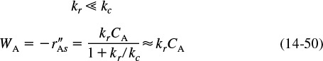
Reaction Rate Limited
The specific reaction rate is independent of the velocity of fluid and for the solid sphere considered here, independent of particle size. However, for porous catalyst pellets, kr may depend on particle size for certain situations, as shown in Chapter 15. We will continue this discussion in Section 14.5.
Mass transfer effects are not important when the reaction rate is limiting.
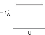
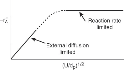
Figure 14-5 shows the variation in reaction rate with Term 2 in Equation (14-49), the ratio of velocity to particle size. At low velocities, the mass transfer boundary-layer thickness is large and diffusion limits the reaction. As the velocity past the sphere is increased, the boundary-layer thickness decreases, and the mass transfer across the boundary layer no longer limits the rate of reaction. One also notes that for a given (i.e., fixed) velocity, reaction-limiting conditions can be achieved by using very small particles. However, the smaller the particle size, the greater the pressure drop in a packed bed. When one is obtaining reaction-rate data in the laboratory, one must operate at sufficiently high velocities or sufficiently small particle sizes to ensure that the reaction is not mass transfer–limited when collecting data.

When collecting rate-law data, operate in the reaction-limited region.
14.4.3 Mass Transfer–Limited Reactions in Packed Beds
A number of industrial reactions are potentially mass transfer–limited because they may be carried out at high temperatures without the occurrence of undesirable side reactions. In mass transfer–dominated reactions, the surface reaction is so rapid that the rate of transfer of reactant from the bulk gas or liquid phase to the surface limits the overall rate of reaction. Consequently, mass transfer–limited reactions respond quite differently to changes in temperature and flow conditions than do the rate-limited reactions discussed in previous chapters. In this section the basic equations describing the variation of conversion with the various reactor design parameters (catalyst weight, flow conditions) will be developed. To achieve this goal, we begin by carrying out a mole balance on the following generic mass transfer–limited reaction
carried out in a packed-bed reactor (Figure 14-6). A steady-state mole balance on reactant A in the reactor segment between z and z + Δz is


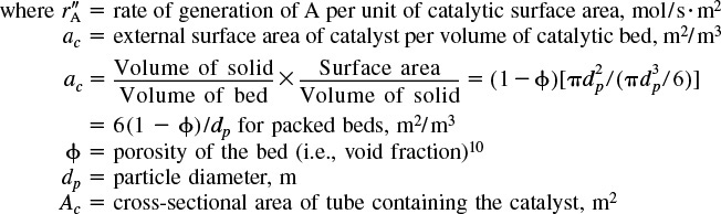
10 In the nomenclature for Chapter 4, for the Ergun equation for pressure drop.
Dividing Equation (14-51) by Ac Δz and taking the limit as Δz → 0, we have
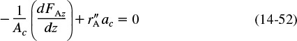
We now need to express FAz and ![]() in terms of concentration.
in terms of concentration.
The molar flow rate of A in the axial direction is
In almost all situations involving flow in packed-bed reactors, the amount of material transported by diffusion or dispersion in the axial direction is negligible compared with that transported by convection (i.e., bulk flow)
Axial diffusion is neglected.
(In Chapter 18 we consider the case when dispersive effects (e.g., diffusion) must be taken into account.) Neglecting dispersion, Equation (14-14) becomes
where U is the superficial molar average velocity through the bed (m/s). Substituting for FAz in Equation (14-52) gives us
For the case of constant superficial velocity U
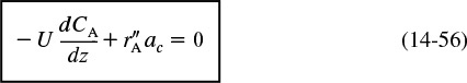
Differential equation describing flow and reaction in a packed bed
For reactions at steady state, the molar flux of A to the particle surface, WAr (mol/m2 · s) (see Figure 14-7), is equal to the rate of disappearance of A on the surface –![]() (mol/m2 · s); that is
(mol/m2 · s); that is
From Section 14.4, the boundary condition at the external surface is
Substituting for ![]() in Equation (14-56), we have
in Equation (14-56), we have
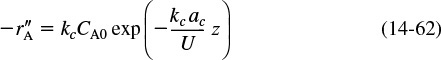
In reactions that are completely mass transfer–limited, it is not necessary to know the rate law.
In most mass transfer–limited reactions, the surface concentration is negligible with respect to the bulk concentration (i.e., ![]() )
)
Integrating with the limit, at z = 0, CA = CA0

The corresponding variation of reaction rate along the length of the reactor is
The concentration and conversion profiles down a reactor of length L are shown in Figure 14-8.
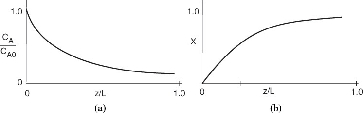
Reactor concentration profile for a mass transfer–limited reaction
To determine the reactor length L necessary to achieve a conversion X, we combine the definition of conversion
with the evaluation of Equation (14-61) at z = L to obtain
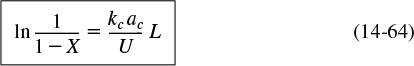
14.4.4 Robert the Worrier
Robert is an engineer who is always worried (which is a Jofostanian trait). He thinks something bad will happen if we change an operating condition such as flow rate or temperature or an equipment parameter such as particle size. Robert’s motto is “If it ain’t broke, don’t fix it.” We can help Robert be a little more adventuresome by analyzing how the important parameters vary as we change operating conditions in order to predict the outcome of such a change. We first look at Equation (14-64) and see that conversion depends upon the parameters kc, ac, U, and L. We now examine how each of these parameters will change as we change operating conditions. We first consider the effects of temperature and flow rate on conversion.

To learn the effect of flow rate on conversion, we need to know how flow rate affects the mass transfer coefficient. That is, we must determine the correlation for the mass transfer coefficient for the particular geometry and flow field. For flow through a packed bed, the correlation given by Thoenes and Kramers for 0.25 < ϕ < 0.5, 40 < Re′ < 4000, and 1 < Sc < 4000 is11
11 D. Thoenes, Jr. and H. Kramers, Chem. Eng. Sci., 8, 271 (1958).
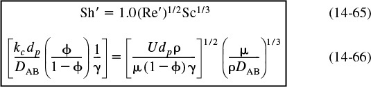
Thoenes–Kramers correlation for flow through packed beds

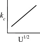
For constant fluid properties and particle diameter
We see that the mass transfer coefficient increases with the square root of the superficial velocity through the bed. Therefore, for a fixed concentration, CA, such as that found in a differential reactor, the rate of reaction should vary with U1/2
For diffusion-limited reactions, reaction rate depends on particle size and fluid velocity.
However, if the gas velocity is continually increased, a point is reached where the reaction becomes reaction rate–limited and, consequently, is independent of the superficial gas velocity, as shown in Figure 14-5.
Most mass transfer correlations in the literature are reported in terms of the Colburn J factor (i.e., JD) as a function of the Reynolds number. The relationship between JD and the numbers we have been discussing is

Colburn J factor
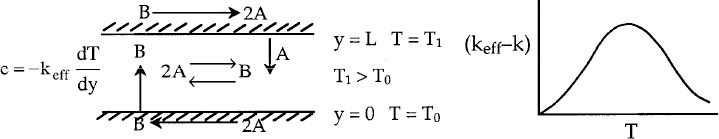
Figure 14-9 shows data from a number of investigations for the J factor as a function of the Reynolds number for a wide range of particle shapes and gas-flow conditions. Note: There are serious deviations from the Colburn analogy when the concentration gradient and temperature gradient are coupled, as shown by Venkatesan and Fogler.12
12 R. Venkatesan and H. S. Fogler, AIChE J., 50, 1623 (July 2004).
Dwidevi and Upadhyay review a number of mass transfer correlations for both fixed and fluidized beds and arrive at the following correlation, which is valid for both gases (Re > 10) and liquids (Re > 0.01) in either fixed or fluidized beds:13
13 P. N. Dwidevi and S. N. Upadhyay, Ind. Eng. Chem. Process Des. Dev., 16, 157 (1977).

A correlation for flow through packed beds in terms of the Colburn J factor
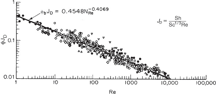
Figure 14-9 Mass transfer correlation for packed beds. ϕb≡ϕ [Reprinted by permission. Copyright © 1977, American Chemical Society. Dwivedi, P. N. and S. N. Upadhyay, “Particle-Fluid Mass Transfer in Fixed and Fluidized Beds.” Industrial & Engineering Chemistry Process Design and Development, 1977, 16 (2), 157–165.]
For nonspherical particles, the equivalent diameter used in the Reynolds and Sherwood numbers is ![]() , where Ap is the external surface area of the pellet.
, where Ap is the external surface area of the pellet.
To obtain correlations for mass transfer coefficients for a variety of systems and geometries, see either D. Kunii and O. Levenspiel, Fluidization Engineering, 2nd ed. (Butterworth-Heinemann, 1991), Chap. 7, or W. L. McCabe, J. C. Smith, and P. Harriott, Unit Operations in Chemical Engineering, 6th ed. (New York: McGraw-Hill, 2000). For other correlations for packed beds with different packing arrangements, see I. Colquhoun-Lee and J. Stepanek, Chemical Engineer, 108 (Feb. 1974).
Example 14–2 Mass Transfer Effects in Maneuvering a Space Satellite
Hydrazine has been studied extensively for use in monopropellant thrusters for space flights of long duration. Thrusters are used for altitude control of communication satellites. Here, the decomposition of hydrazine over a packed bed of alumina-supported iridium catalyst is of interest.14 In a proposed study, a 2% hydrazine in 98% helium mixture is to be passed over a packed bed of cylindrical particles 0.25 cm in diameter and 0.5 cm in length at a gas-phase velocity of 150 m/s and a temperature of 450 K. The kinematic viscosity of helium at this temperature is 4.94 × 10⁻⁵ m2/s. The hydrazine decomposition reaction is believed to be externally mass transfer–limited under these conditions. If the packed bed is 0.05 m in length, what conversion can be expected? Assume isothermal operation.
14 O. I. Smith and W. C. Solomon, Ind. Eng. Chem. Fund., 21, 374.

Actual case history and current application
DAB = 0.69 × 10⁻⁴ m2/s at 298 K
Bed porosity: 40%
Bed fluidicity: 95.7%
Solution
The following solution is detailed and a bit tedious, but it is important to know the details of how a mass transfer coefficient is calculated. Rearranging Equation (14-64) gives us

Tedious reading and calculations, but we gotta know how to do the nitty–gritty.
(a) Using the Thoenes–Kramers correlation to calculate the mass transfer coefficient, kc
1. First we find the volume-average particle diameter

2. Surface area per volume of bed
3. Mass transfer coefficient
For cylindrical pellets

Representative values
Correcting the diffusivity to 450 K using Table 14-2 gives us

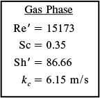
Substituting Re’ and Sc into Equation (14-65) yields
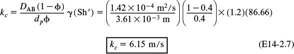
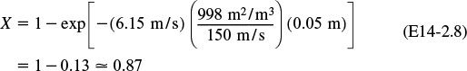
We find 87% conversion.
(b) Colburn JD factor to calculate kc. To find kc, we first calculate the surface-area-average particle diameter.
Once again the nitty-gritty
For cylindrical pellets, the external surface area is

Typical values

Fluidicity?? Red herring!
If there were such a thing as the bed fluidicity, given in the problem statement, it would be a useless piece of information. Make sure that you know what information you need to solve problems, and go after it. Do not let additional data confuse you or lead you astray with useless information or facts that represent someone else’s bias, and which are probably not well founded.
14.5 What If . . . ? (Parameter Sensitivity)
As we have stressed many times, one of the most important skills of an engineer is to be able to predict the effects of changes of system variables on the operation of a process. The engineer needs to determine these effects quickly through approximate but reasonably close calculations, which are sometimes referred to as “back-of-the-envelope calculations.”15 This type of calculation is used to answer such questions as “What will happen if I decrease the particle size?” “What if I triple the flow rate through the reactor?”
15 Prof. J. D. Goddard, University of Michigan, 1963–1976. Currently at University of California, San Diego.
J. D. Goddard’s
Back of the Envelope
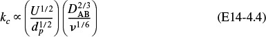
To help answer these questions, we recall Equation (14-49) and our discussion on page 696. There, we showed the mass transfer coefficient for a packed bed was related to the product of two terms: Term 1 was dependent on the physical properties and Term 2 was dependent on the system properties. Re-writing Equation (14-41) as
one observes from this equation that the mass transfer coefficient increases as the particle size decreases. The use of sufficiently small particles offers another technique to escape from the mass transfer–limited regime into the reaction-rate-limited regime.
Find out how the mass transfer coefficient varies with changes in physical properties and system properties.
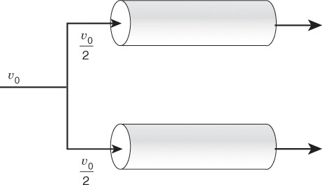
Example 14–3 The Case of Divide and Be Conquered
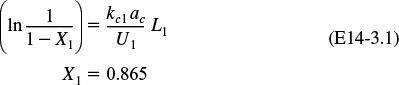
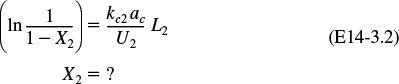
A mass transfer–limited reaction is being carried out in two reactors of equal volume and packing, connected in series as shown in Figure E14-3.1. Currently, 86.5% conversion is being achieved with this arrangement. It is suggested that the reactors be separated and the flow rate be divided equally among each of the two reactors (Figure E14-3.2) to decrease the pressure drop and hence the pumping requirements. In terms of achieving a higher conversion, Robert is wondering if this is a good idea.

Reactors in series versus reactors in parallel
For the series arrangement we were given, X1 = 0.865, and for the parallel arrangement, the conversion is unknown, i.e., X2 = ? As a first approximation, we neglect the effects of small changes in temperature and pressure on mass transfer. We recall Equation (14-64), which gives conversion as a function of reactor length. For a mass transfer–limited reaction
For case 1, the undivided system
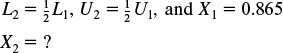
For case 2, the divided system
We now take the ratio of case 2 (divided system) to case 1 (undivided system)
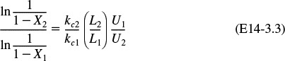
The surface area per unit volume ac is the same for both systems.
From the conditions of the problem statement we know that
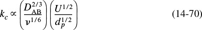
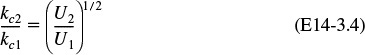
However, we must also consider the effect of the division on the mass transfer coefficient. From Equation (14-70) we know that
kc ∝ U1/2
Then
Multiplying by the ratio of superficial velocities yields
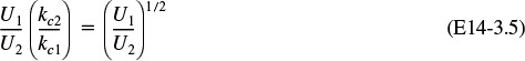
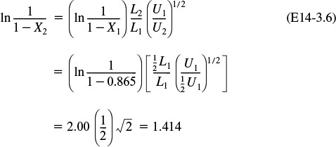
X2 = 0.76
Analysis: Consequently, we see that although the divided arrangement will have the advantage of a smaller pressure drop across the bed, it is a bad idea in terms of conversion. Recall that the series arrangement gave X1 = 0.865; therefore (X2 < X1). Bad idea!! But every chemical engineering student in Jofostan knew that! Recall that if the reaction were reaction rate–limited, both arrangements would give the same conversion.
Bad idea!! Robert was right to worry.
Example 14–4 The Case of the Overenthusiastic Engineers
The same reaction as that in Example 14-3 is being carried out in the same two reactors in series. A new engineer suggests that the rate of reaction could be increased by a factor of 210 by increasing the reaction temperature from 400°C to 500°C, reasoning that the reaction rate doubles for every 10°C increase in temperature. Another engineer arrives on the scene and berates the new engineer with quotations from Chapter 3 concerning this rule of thumb. She points out that it is valid only for a specific activation energy within a specific temperature range. She then suggests that he go ahead with the proposed temperature increase but should only expect an increase on the order of 23 or 24. What do you think? Who is correct?
Robert worries if this temperature increase will be worth the trouble.
Solution
Because almost all surface reaction rates increase more rapidly with temperature than do diffusion rates, increasing the temperature will only increase the degree to which the reaction is mass transfer–limited.
We now consider the following two cases:
![]()
Taking the ratio of case 2 to case 1 and noting that the reactor length is the same for both cases (L1 = L2), we obtain

The molar feed rate FT0 remains unchanged
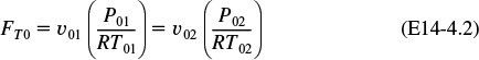
the pressure remains constant so
Because υ = Ac U, the superficial velocity at temperature T2 is
We now wish to learn the dependence of the mass transfer coefficient on temperature
Taking the ratio of case 2 to case 1 and realizing that the particle diameter is the same for both cases gives us

The temperature dependence of the gas-phase diffusivity is (from Table 14-2)
For most gases, viscosity increases with increasing temperature according to the relation

It’s really important to know how to do this type of analysis.
Rearranging Equation (E14-4.1) in the form

Analysis: Consequently, we see that increasing the temperature from 400°C to 500°C increases the conversion by only 1.7%, i.e., X = 0.865 compared to X = 0.88. Bad idea! Bad, bad idea! Both engineers would have benefited from a more thorough study of this chapter.
Bad idea!! Robert was right to worry.
For a packed catalyst bed, the temperature-dependence part of the mass transfer coefficient for a gas-phase reaction can be written as

Important concept
Depending on how one fixes or changes the molar feed rate, FT0, U may also depend on the feed temperature. As an engineer, it is extremely important that you reason out the effects of changing conditions, as illustrated in the preceding two examples.
Summary
1. The molar flux of A in a binary mixture of A and B is
a. For equimolar counterdiffusion (EMCD) or for dilute concentration of the solute
b. For diffusion through a stagnant gas
2. The rate of mass transfer from the bulk fluid to a boundary at concentration CAs is
where kc is the mass transfer coefficient.
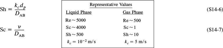
3. The Sherwood and Schmidt numbers are, respectively,
4. If a heat transfer correlation exists for a given system and geometry, the mass transfer correlation may be found by replacing the Nusselt number by the Sherwood number and the Prandtl number by the Schmidt number in the existing heat transfer correlation.
5. Increasing the gas-phase velocity and decreasing the particle size will increase the overall rate of reaction for reactions that are externally mass transfer–limited.
6. The conversion for externally mass transfer–limited reactions can be found from the equation
7. Back-of-the-envelope calculations should be carried out to determine the magnitude and direction that changes in process variables will have on conversion. What if . . .?
1. Transdermal Drug Delivery

2. Shrinking Core Model
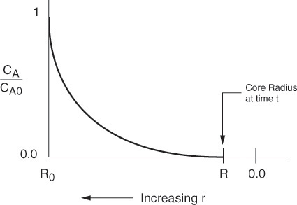
Figure 11-14 Oxygen concentration profile shown from the external radius of the pellet (R0) to the pellet center. The gas–carbon interface is located at R.
3. Diffusion through Film to a Catalyst Particle
4. WP14-(a) Revisit Transdermal Drug Delivery
5. Additional Homework Problems
• Learning Resources
1. Summary Notes
Diffusion through a Stagnant Film
4. Solved Problems
Example CD14-1 Calculating Steady State Diffusion
Example CD14-2 Relative Fluxes WA, BA, and JA
Example CD14-3 Diffusion through a Stagnant Gas
Example CD14-4 Measuring Gas-Phase Diffusivities
Example CD14-5 Diffusion through a Film to a Catalyst Particle
Example CD14-6 Measuring Liquid-Phase Diffusivities
• Professional Reference Shelf
R14.1. Mass Transfer-Limited Reactions on Metallic Surfaces
A. Catalyst Monoliths
B. Wire Gauze Reactors
R14.2. Methods to Experimentally Measure Diffusivities

R14.3. Facilitated Heat Transfer
R14.4. Shrinking Core Model
R14.5. Dissolution of Monodisperse Particles
R14.6. Dissolution of Polydisperse Solids (e.g., pills in the stomach)

Questions and Problems
The subscript to each of the problem numbers indicates the level of difficulty: A, least difficult; D, most difficult.
Questions
Q14-1 Read over the problems at the end of this chapter. Make up an original problem that uses the concepts presented in this chapter. See problem P5-1A for the guidelines. To obtain a solution:
(a) Make up your data and reaction.
(b) Use a real reaction and real data.
The journals listed at the end of Chapter 1 may be useful for part (b).

Q14-2 (Seargeant Amberrcromby). Capt. Apollo is piloting a shuttlecraft on his way to space station Klingon. Just as he is about to maneuver to dock his craft using the hydrazine system discussed in Example 14-2, the shuttle craft’s thrusters do not respond properly and it crashes into the station, killing Capt. Apollo (Star Wars 7 (fall 2015)). An investigation reveals that Lt. Darkside prepared the packed beds used to maneuver the shuttle and Lt. Data prepared the hydrazine-helium gas mixture. Foul play is suspected and Sgt. Ambercromby arrives on the scene to investigate.
(a) What are the first three questions he asks?
(b) Make a list of possible explanations for the crash, supporting each one by an equation or reason.
(a) Example 14-1. How would your answers change if the temperature was increased by 50°C, the particle diameter was doubled, and fluid velocity was cut in half? Assume properties of water can be used for this system.
(b) Example 14-2. How would your answers change if you had a 50–50 mixture of hydrazine and helium? If you increase dp by a factor of 5?
(c) Example 14-3. What if you were asked for representative values for Re, Sc, Sh, and kc for both liquid- and gas-phase systems for a velocity of 10 cm/s and a pipe diameter of 5 cm (or a packed-bed diameter of 0.2 cm)? What numbers would you give?
(d) Example 14-4. How would your answers change if the reaction were carried out in the liquid phase where kinematic viscosity varied as ![]() ?
?
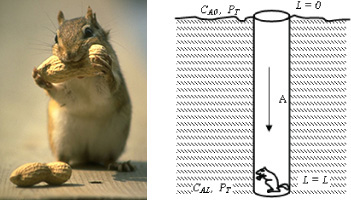
P14-2B Assume the minimum respiration rate of a chipmunk is 1.5 micromoles of O2/min. The corresponding volumetric rate of gas intake is 0.05 dm3/min at STP.
(a) What is the deepest a chipmunk can burrow a 3-cm diameter hole beneath the surface in Ann Arbor, Michigan? DAB = 1.8 × 10⁻⁵ m2/s
(b) In Boulder, Colorado?
(c) How would your answers to (a) and (b) change in the dead of winter when T = 0°F?
(d) Critique and extend this problem (e.g., CO2 poisoning). Thanks to Professor Robert Kabel at Pennsylvania State University.
Hint: Review derivations and equations for WA and WB to see how they can be applied to this problem.
P14-3B Pure oxygen is being absorbed by xylene in a catalyzed reaction in the experimental apparatus sketched in Figure P14-3B. Under constant conditions of temperature and liquid composition, the following data were obtained:
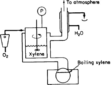

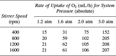
No gaseous products were formed by the chemical reaction. What would you conclude about the relative importance of liquid-phase diffusion and about the order of the kinetics of this reaction? (California Professional Engineers Exam)
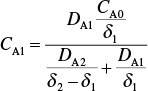
P14-4C In a diving-chamber experiment, a human subject breathed a mixture of O2 and He while small areas of his skin were exposed to nitrogen gas. After some time, the exposed areas became blotchy, with small blisters forming on the skin. Model the skin as consisting of two adjacent layers, one of thickness δ1 and the other of thickness δ2. If counterdiffusion of He out through the skin occurs at the same time as N2 diffuses into the skin, at what point in the skin layers is the sum of the partial pressures a maximum? If the saturation partial pressure for the sum of the gases is 101 kPa, can the blisters be a result of the sum of the gas partial pressures exceeding the saturation partial pressure and the gas coming out of the solution (i.e., the skin)?

Before answering any of these questions, derive the concentration profiles for N2 and He in the skin layers.
Diffusivity of He and N2 in the inner skin layer = 5 × 10⁻⁷ cm2/s and 1.5 × 10⁻⁷ cm2/s, respectively
Diffusivity of He and N2 in the outer skin layer = 10–5 cm2/s and 3.3 × 10⁻⁴ cm2/s, respectively

Hint: See Transdermal Drug Delivery in Expanded Material on the CRE Web site.
P14-5B The decomposition of cyclohexane to benzene and hydrogen is mass transfer–limited at high temperatures. The reaction is carried out in a 5-cm-ID pipe 20 m in length packed with cylindrical pellets 0.5 cm in diameter and 0.5 cm in length. The pellets are coated with the catalyst only on the outside. The bed porosity is 40%. The entering volumetric flow rate is 60 dm3/min.
(a) Calculate the number of pipes necessary to achieve 99.9% conversion of cyclohexane from an entering gas stream of 5% cyclohexane and 95% H2 at 2 atm and 500°C.
(b) Plot conversion as a function of pipe length.
(c) How much would your answer change if the pellet diameter and length were each cut in half?
(d) How would your answer to part (a) change if the feed were pure cyclohexane?
(e) What do you believe is the point of this problem? Is the focus really green CRE? How so?

Green engineering
P14-6C Lead titanate, PbTiO3, is a material having remarkable ferroelectric, pyroelectric, and piezoelectric properties [J. Elec. Chem. Soc., 135, 3137 (1988)]. A thin film of PbTiO3 was deposited in a CVD reactor. The deposition rate is given below as a function of a temperature and flow rate over the film.
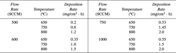
What are all the things, qualitative and quantative, that you can learn from these data?
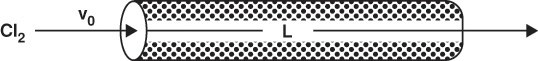
P14-7B A plant is removing a trace of Cl2 from a waste-gas stream by passing it over a solid granulm absorbent in a tubular packed bed (Figure P14-7). At present, 63.2% removal is being acomplished, but it is believed that greater removal could be achieved if the flow rate were increased by a factor of 4, the particle diameter were decreased by a factor of 3, and the packed tube length increased by 50%. What percentage of chlorine would be removed under the proposed scheme? (The chlorine transferring to the absorbent is removed completely by a virtually instantaneous chemical reaction.) (Ans.: 98%)
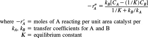
P14-8B In a certain chemical plant, a reversible fluid-phase isomerization
is carried out over a solid catalyst in a tubular packed-bed reactor. If the reaction is so rapid that mass transfer between the catalyst surface and the bulk fluid is rate-limiting, show that the kinetics are described in terms of the bulk concentrations CA and CB by
It is desired to double the capacity of the existing plant by processing twice the feed of reactant A while maintaining the same fractional conversion of A to B in the reactor. How much larger a reactor, in terms of catalyst weight, would be required if all other operating variables are held constant? You may use the Thoenes–Kramers correlation for mass transfer coefficients in a packed bed.
P14-9B The irreversible gas-phase reaction
is carried out adiabatically over a packed bed of solid catalyst particles. The reaction is first order in the concentration of A on the catalyst surface
The feed consists of 50% (mole) A and 50% inerts, and enters the bed at a temperature of 300 K. The entering volumetric flow rate is 10 dm3/s (i.e., 10,000 cm3/s). The relationship between the Sherwood number and the Reynolds number is
Sh = 100 Re1/2
As a first approximation, one may neglect pressure drop. The entering concentration of A is 1.0 M. Calculate the catalyst weight necessary to achieve 60% conversion of A for
(a) isothermal operation.
(b) adiabatic operation.
Additional information:
Kinematic viscosity: μ/ρ = 0.02 cm2/s
Particle diameter: dp = 0.1 cm
Superficial velocity: U = 10 cm/s
Catalyst surface area/mass of catalyst bed: a = 60 cm2/g-cat
Diffusivity of A: De = 10–2 cm2/s
Heat of reaction: ![]() = –10,000 cal/g mol A
= –10,000 cal/g mol A
Heat capacities: CpA = CpB = 25 cal/g mol · K, C pS (solvent) = 75 cal/g mol · K
k′ (300 K) 0.01 cm3/s ·g-cat with E 4000 cal/mol
P14-10B Transdermal Drug Delivery. See photo on page 713. The principles of steady-state diffusion have been used in a number of drug-delivery systems. Specifically, medicated patches are commonly attached to the skin to deliver drugs for nicotine withdrawal, birth control, and motion sickness, to name a few. The U.S. transdermal drug-delivery is a multi-billion dollar market. Equations similar to Equation (14-24) have been used to model the release, diffusion, and absorption of the drug from the patch into the body. The figure shown in the Expanded Material on page 713 shows a drug-delivery vehicle (patch) along with the concentration gradient in the epidermis and dermis skin layers.
(a) Use a shell balance to show
(b) Show the concentration profile in the epidermis layer
(c) Show the concentration profile in the dermis layer
(d) Equate the fluxes using ![]() and
and ![]() at z = δ1 to show
at z = δ1 to show
(e) What are the concentration profiles in the dermis and epidermis layers?
(f) Show the flux in the dermis layer is
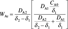
(g) What is the flux in the epidermis layer?
P14-11D (Estimating glacial ages) The following oxygen-18 data were obtained from soil samples taken at different depths in Ontario, Canada. Assuming that all the 18O was laid down during the last glacial age and that the transport of 18O to the surface takes place by molecular diffusion, estimate the number of years since the last glacial age from the following data. Independent measurements give the diffusivity of 18O in soil as 2.64 × 10⁻¹⁰ m2/s.
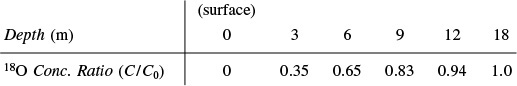
C0 is the concentration of 18O at 25 m. Hint: A knowledge of error function solutions may or may not be helpful. (Ans.: t = 5,616 years)
Journal Critique Problems
P14C-1 The decomposition of nitric oxide on a heated platinum wire is discussed in Chem. Eng. Sci., 30, 781. After making some assumptions about the density and the temperatures of the wire and atmosphere, and using a correlation for convective heat transfer, determine if mass transfer limitations are a problem in this reaction.
Supplementary Reading
1. The fundamentals of diffusional mass transfer may or may not be found in
BIRD, R. B., W. E. STEWART, and E. N. LIGHTFOOT, Transport Phenomena, 2nd ed. New York: Wiley, 2002, Chaps. 17 and 18.
Collins, S., Mockingjay (The Final Book of the Hunger Games). New York: Scholastic, 2014.
CUSSLER, E. L., Diffusion Mass Transfer in Fluid Systems, 3rd ed. New York: Cambridge University Press, 2009.
GEANKOPLIS, C. J., Transport Processes and Unit Operations. Upper Saddle River, NJ: Prentice Hall, 2003.
LEVICH, V. G., Physiochemical Hydrodynamics. Upper Saddle River, NJ: Prentice Hall, 1962, Chaps. 1 and 4.
2. Experimental values of the diffusivity can be found in a number of sources, two of which are
PERRY, R. H., D. W. GREEN, and J. O. MALONEY, Chemical Engineers’ Handbook, 8th ed. New York: McGraw-Hill, 2007.
SHERWOOD, T. K., R. L. PIGFORD, and C. R. WILKE, Mass Transfer. New York: McGraw-Hill, 1975.
3. A number of correlations for the mass transfer coefficient can be found in
LYDERSEN, A. L., Mass Transfer in Engineering Practice. New York: Wiley-Interscience, 1983, Chap. 1.
MCCABE, W. L., J. C. SMITH, and P. HARRIOTT, Unit Operations of Chemical Engineering, 6th ed. New York: McGraw-Hill, 2000, Chap. 17.