
Solutions to Selected Problems
Solutions for Column 1
1. This C program uses the Standard Library qsort to sort a file of integers.
int intcomp(int *x, int *y)
{ return *x - *y; }
int a[1000000];
int main(void)
{ int i, n=0;
while (scanf("%d", &a[n]) != EOF)
n++;
qsort(a, n, sizeof(int), intcomp);
for (i = 0; i < n; i++)
printf("%d
", a[i]);
return 0;
}
This C++ program uses the set container from the Standard Template Library for the same job.
int main(void)
{ set<int> S;
int i;
set<int>::iterator j;
while (cin >> i)
S.insert(i);
for (j = S.begin(); j != S.end(); ++j)
cout << *j << "
";
return 0;
}
Solution 3 sketches the performance of both programs.
2. These functions use the constants to set, clear and test the value of a bit:
#define BITSPERWORD 32
#define SHIFT 5
#define MASK OxlF
#define N 10000000
int a[l + N/BITSPERWORD]:
void set(int i) { a[i>>SHIFT] |= (l<<(i & MASK)); }
void clr(int i) { a[i>>SHIFT] &= ~(l<<(i & MASK)); }
int test(int i){ return a[i>>SHIFT] & (l<<(i & MASK)); }
3. This C code implements the sorting algorithm, using the functions defined in Solution 2.
int main(void)
{ int i;
for (i = 0; i < N; i++)
clr(i);
while (scanf("%d", &i) != EOF)
set(i);
for (i = 0; i < N; i++)
if (test(i))
printf("%d
", i);
return 0;
}
I used the program in Solution 4 to generate a file of one million distinct positive integers, each less than ten million. This table reports the cost of sorting them with the system command-line sort, the C++ and C programs in Solution 1, and the bitmap code:
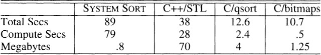
The first line reports the total time, and the second line subtracts out the 10.2 seconds of input/output required to read and write the files. Even though the general C++ program uses 50 times the memory and CPU time of the specialized C program, it requires just half the code and is much easier to extend to other problems.
4. See Column 12, especially Problem 12.8. This code assumes that randint(l, u) returns a random integer in l..u.
for i = [0, n)
x[i] = i
for i = [0, k)
swap(i, randint(i, n-1))
print x[i]
The swap function exchanges the two elements in x. The randint function is discussed in detail in Section 12.1.
5. Representing all ten million numbers with a bitmap requires that many bits, or 1.25 million bytes. Employing the fact that no phone numbers begin with the digits zero or one reduces the memory to exactly one million bytes. Alternatively, a two-pass algorithm first sorts the integers 0 through 4,999,999 using 5,000,000/8 = 625,000 words of storage, then sorts 5,000,000 through 9,999,999 in a second pass. A k-pass algorithm sorts at most n nonrepeated positive integers less than n in time kn and space n/k.
6. If each integer appears at most ten times, then we can count its occurrences in a four-bit half-byte (or nybble). Using the solution to Problem 5, we can sort the complete file in a single pass with 10,000,000/2 bytes, or in k passes with 10,000,000/2k bytes.
9. The effect of initializing the vector data[0..n – 1 ] can be accomplished with a signature contained in two additional n-element vectors, from and to, and an integer top. If the element data[i] has been initialized, then from[i]<top and to[from[i]] = i. Thus from is a simple signature, and to and top together make sure that from is not accidentally signed by the random contents of memory. Blank entries of data are uninitialized in this picture:

The variable top is initially zero; the array element i is first accessed by the code
from[i] = top
to[top] = i
data[i] = 0
top++
This problem and solution are from Exercise 2.12 of Aho, Hopcroft and Ullman’s Design and Analysis of Computer Algorithms, published by Addison-Wesley in 1974. It combines key indexing and a wily signature scheme. It can be used for matrices as well as vectors.
10. The store placed the paper order forms in a 10×10 array of bins, using the last two digits of the customer’s phone number as the hash index. When the customer telephoned an order, it was placed in the proper bin. When the customer arrived to retrieve the merchandise, the salesperson sequentially searched through the orders in the appropriate bin — this is classical “open hashing with collision resolution by sequential search”. The last two digits of the phone number are quite close to random and therefore an excellent hash function, while the first two digits would be a horrible hash function — why? Some municipalities use a similar scheme to record deeds in sets of record books.
11. The computers at the two facilities were linked by microwave, but printing the drawings at the test base would have required a printer that was very expensive at the time. The team therefore drew the pictures at the main plant, photographed them, and sent 35mm film to the test station by carrier pigeon, where it was enlarged and printed photographically. The pigeon’s 45-minute flight took half the time of the car, and cost only a few dollars per day. During the 16 months of the project the pigeons transmitted several hundred rolls of film, and only two were lost (hawks inhabit the area; no classified data was carried). Because of the low price of modern printers, a current solution to the problem would probably use the microwave link.
12. According to the urban legend, the Soviets solved their problem with a pencil, of course. For background on the true story, see www.spacepen.com. The Fisher Space Pen company was founded in 1948, and its writing instruments have been used by the Russian Space Agency, underwater explorers, and Himalayan climbing expeditions.
Solutions for Column 2
A. It is helpful to view this binary search in terms of the 32 bits that represent each integer. In the first pass of the algorithm we read the (at most) four billion input integers and write those with a leading zero bit to one sequential file and those with a leading one bit to another file.

One of those two files contains at most two billion integers, so we next use that file as the current input and repeat the probe process, but this time on the second bit. If the original input file contains n elements, the first pass will read n integers, the second pass at most n/2, the third pass at most n/4, and so on, so the total running time is proportional to n. The missing integer could be found by sorting the file and then scanning, but that would require time proportional to n log n. This problem was given as an exam by Ed Reingold at the University of Illinois.
B. See Section 2.3.
C. See Section 2.4.
1. To find all anagrams of a given word we first compute its signature. If no preprocessing is allowed then we have to read the entire dictionary sequentially, compute the signature of each word, and compare the two signatures. With preprocessing, we could perform a binary search in a precomputed structure containing (signature, word) pairs sorted by signature. Musser and Saini implement several anagram programs in Chapters 12 through 15 of their STL Tutorial and Reference Guide, published by Addison-Wesley in 1996.
2. Binary search finds an element that occurs at least twice by recursively searching the subinterval that contains more than half of the integers. My original solution did not guarantee that the number of integers is halved in each iteration, so the worst-case run time of its log2 n passes was proportional to n log n. Jim Saxe reduced that to linear time by observing that the search can avoid carrying too many duplicates. When his search knows that a duplicate must be in a current range of m integers, it will only store m +1 integers on its current work tape; if more integers would have gone on the tape, his program discards them. Although his method frequently ignores input variables, its strategy is conservative enough to ensure that it finds at least one duplicate.
3. This “juggling” code rotates x[n] left by rotdist.
for i = [0, gcd(rotdist, n))
/* move i-th values of blocks */
t = x[i]
j = i
loop
k = j + rotdist
if k >= n
k -= n
if k == i
break
x[j] = x[k]
j = k
x[j] = t
The greatest common divisor of rotdist and n is the number of cycles to be permuted (in terms of modern algebra, it is the number of cosets in the permutation group induced by the rotation).
The next program is from Section 18.1 of Goes’s Science of Programming; it assumes that the function swap (a, b, m) exchanges x[a..a + m – l] with x[b..b + m – 1].
if rotdist == 0 || rotdist == n
return
i = p = rotdist
j = n - p
while i != j
/* invariant:
x[0 ..p-i ] in final position
x[p-i..p-1 ] = a (to be swapped with b)
x[p ..p+j-1] = b (to be swapped with a)
x[p+j..n-1 ] in final position
*/
if i > j
swap(p-i, p, j)
i -= j
else
swap(p-i, p+j-i, i)
j -= i
swap(p-i, p, i)
Loop invariants are described in Column 4.
The code is isomorphic to this (slow but correct) additive Euclidean algorithm for computing the greatest common divisor of i and j, which assumes that neither input is zero.
int gcd(int i, int j)
while i != j
if i > j
i -= j
else
j -= i
return i
Gries and Mills study all three rotation algorithms in “Swapping Sections”, Cornell University Computer Science Technical Report 81-452.
4. I ran all three algorithms on a 400MHz Pentium II, with n fixed at 1,000,000 and the rotation distance varying from 1 to 50. This graph plots the average time of 50 runs at each data set:

The reversal code has a consistent run time of about 58 nanoseconds per element, except that the time jumps to about 66 for rotation distances of 4, 12, 20 and all later integers congruent to 4 modulo 8. (This is probably an interaction with a cache size of 32 bytes.) The block swap algorithm starts off as the most expensive algorithm (probably due to a function call for swapping single-element blocks), but its good caching behavior makes it the fastest for rotation distances greater than 2. The juggling algorithm starts as the cheapest, but its poor caching behavior (accessing a single element from each 32-byte cache line) drives its time to near 200 nanoseconds at a rotation distance of 8. Its time hovers around 190 nanoseconds, and drops down sporadically (at a rotation distance of 1000, its time drops to 105 nanoseconds, then pops right back up to 190). In the mid 1980’s, this same code tickled paging behavior with the rotation distance set to the page size.
6. The signature of a name is its push-button encoding, so the signature of “LESK*M*” is “5375*6*”. To find the false matches in a directory, we sign each name with its push-button encoding, sort by signature (and by name within equal signatures), and then sequentially read the sorted file to report any equal signatures with distinct names. To retrieve a name given its push-button encoding we use a structure that contains the signatures and the other data. While we could sort that structure and then look up a push-button encoding by binary search, in a real system we would probably use hashing or a database system.
7. To transpose the row-major matrix, Vyssotsky prepended the column and row to each record, called the system tape sort to sort by column then row, and then removed the column and row numbers with a third program.
8. The aha! insight for this problem is that some n-element subset sums to at most t if and only if the subset consisting of the k smallest elements does. That subset can be found in time proportional to n log n by sorting the original set, or in time proportional to n by using a selection algorithm (see Solution 11.9). When Ullman assigned this as a class exercise, students designed algorithms with both running times mentioned above, as well as O(n log k), O(nk), O(n2), and O(nk). Can you find natural algorithms to go with those running times?
10. Edison filled the shell with water and emptied it into a graduated cylinder. (As the hint may have reminded you, Archimedes also used water to compute volumes; in his day, aha! insights were celebrated by shouting eureka!)
Solutions for Column 3
1. Each entry in a tax table contains three values: the lower bound for this bracket, the base tax, and the rate at which income over the lower bound is taxed. Including a final sentinel entry in the table with an “infinite” lower bound will make the sequential search easier to write and incidentally faster (see Section 9.2); one could also use a binary search. These techniques apply to any piecewise-linear functions.
3. This block letter “I”
XXXXXXXXX
XXXXXXXXX
XXXXXXXXX
XXX
XXX
XXX
XXX
XXX
XXX
XXXXXXXXX
XXXXXXXXX
XXXXXXXXX
might be encoded as
3 lines 9 X
6 lines 3 blank 3 X 3 blank
3 lines 9 X
or more compactly as
3 9 X
6 3 b 3 X 3 b
3 9 X
4. To find the number of days between two dates, compute the number of each day in its respective year, subtract the earlier from the later (perhaps borrowing from the year), and then add 365 times the difference in years plus one for each leap year.
To find the day of the week for a given day, compute the number of days between the given day and a known Sunday, and then use modular arithmetic to convert that to a day of the week. To prepare a calendar for a month in a given year, we need to know how many days there are in the month (take care to handle February correctly) and the day of the week on which the Ist falls. Dershowitz and Rein-gold wrote an entire book on Calendrical Calculations (published by Cambridge University Press in 1997).
5. Because the comparisons take place from the right to the left of the word, it will probably pay to store the words in reverse (right-to-left) order. Possible representations of a sequence of suffixes include a two-dimensional array of characters (which is usually wasteful), a single array of characters with the suffixes separated by a terminator character, and such a character array augmented with an array of pointers, one to each word.
6. Aho, Kernighan and Weinberger give a nine-line program for generating form letters on page 101 of their Awk Programming Language (published by Addison-Wesley in 1988).
Solutions for Column 4
1. To show that overflow does not occur we add the conditions 0≤l≤n and – 1 ≤u < n to the invariant; we can then bound l + u. The same conditions can be used to show that elements outside the array bounds are never accessed. We can formally define mustbe(l, u) as x[l – l]<t and x[u + l]>t if we define the fictitious boundary elements x[– 1] and x[n] as in Section 9.3.
2. See Section 9.3.
5. For an introduction to this celebrated open problem of mathematics, see B. Hayes’s “On the ups and downs of hailstone numbers” in the Computer Recreations column in the January 1984 Scientific American. For a more technical discussion, see “The 3x+l problem and its generalizations” by J. C. Lagarias, in the January 1985 American Mathematical Monthly. As this book goes to press, Lagarias has a 30-page bibliography with about a hundred references to the problem at www.research.att.com/~jcl/3x+l.html.
6. The process terminates because each step decreases the number of beans in the can by one. It always removes either zero or two white beans from the coffee can, so it leaves invariant the parity (oddness or evenness) of the number of white beans. Thus the last remaining bean is white if and only if the can originally held an odd number of white beans.
7. Because the line segments that form the rungs of the ladder are in increasing y-order, the two that bracket a given point can be found by binary search. The basic comparison in the search tells whether the point is below, on, or above a given line segment; how would you code that function?
8. See Section 9.3.
Solutions for Column 5
1. When I write large programs, I use long names (ten or twenty characters) for my global variables. This column uses short variable names such as x, n and t. In most software projects, the shortest plausible names might be more like elem, nelems and target. I find the short names convenient for building scaffolding and essential for mathematical proofs like that in Section 4.3. Similar rules apply to mathematics: the unfamiliar may want to hear that “the square of the hypotenuse of a right triangle is equal to the sum of the squares of the two adjacent sides”, but people working on the problem usually say “a2 + b2 = c2”.
I’ve tried to stick close to Kernighan and Ritchie’s C coding style, but I put the first line of code with the opening curly brace of a function and delete other blank lines to save space (a substantial percentage, for the little functions in this book).
The binary search in Section 5.1 returns an integer that is – 1 if the value is not present, and points to the value if it is present. Steve McConnell suggested that the search should properly return two values: a boolean telling whether it is present, and an index that is used only if the boolean is true:
boolean BinarySearch(DataType TargetValue, int *TargetIndex)
/* precondition: Element[0] <= Element[l] <=
... <= Element[NumElements-l]
postcondition:
result == false =>
TargetValue not in Element[0..NumElements-l]
result == true =>
Element[*TargetIndex] == TargetValue
*/
Listing 18.3 on page 402 of McConnell’s Code Complete is a Pascal Insertion Sort that occupies one (large) page; the code and comments are together 41 lines. That style is appropriate for large software projects. Section 11.1 of this book presents the same algorithm in just five lines of code.
Few of the programs have error checking. Some functions read data from files into arrays of size MAX, and scanf calls can easily overflow their buffers. Array arguments that should be parameters are instead global variables.
Throughout this book, I’ve used shortcuts that are appropriate for textbooks and scaffolding, but not for large software projects. As Kernighan and Pike observe in Section 1.1 of their Practice of Programming, “clarity is often achieved through brevity”. Even so, most of my code avoids the incredibly dense style illustrated in the C++ code in Section 14.3.
7. For n = 1000, searching through the array in sorted order required 351 nanoseconds per search, while searching it in random order raised the average cost to 418 nanoseconds (about a twenty percent slowdown). For n = 106, the experiment overflows even the L2 cache and the slowdown is a factor of 2.7. For the highly-tuned binary search in Section 8.3, though, the ordered searches zipped right through an n = 1000-element table in 125 nanoseconds each, while the random searches required 266 nanoseconds, a slowdown of over a factor of two.
Solutions for Column 6
4. Want your system to be reliable? Start by building reliability in from the initial design; it is impossible to paste on later. Design your data structures so that information can be recovered if portions of a structure are compromised. Inspect code in reviews and walkthroughs, and test it extensively. Run your software on top of a reliable operating system, and on a redundant hardware system using error-correcting memory. Have in place a plan to recover quickly when your system does fail (and it certainly will fail). Log every failure carefully so that you can learn from each one.
6. “Make it work first before you make it work fast” is usually good advice. However, it took Bill Wulf only a few minutes to convince me that the old truism isn’t quite as true as I once thought. He used the case of a document production system that took several hours to prepare a book. Wulf s clincher went like this: “That program, like any other large system, today has ten known, but minor, bugs. Next month, it will have ten different known bugs. If you could choose between removing the ten current bugs or making the program run ten times faster, which would you pick?”
Solutions for Column 7
These solutions include guesses at constants that may be off by a factor of two from their correct values as this book goes to press, but not much further.
1. The Passaic River does not flow at 200 miles per hour, even when falling 80 feet over the beautiful Great Falls in Paterson, New Jersey. I suspect that the engineer really told the reporter that the engorged river was flowing at 200 miles per day, five times faster than its typical 40 miles per day, which is just under a leisurely 2 miles per hour.
2. An old removable disk holds 100 megabytes. An ISDN line transmits 112 kilobits per second, or about 50 megabytes per hour. This gives a cyclist with a disk in his pocket about two hours to pedal, or a 15-mile radius of superiority. For a more interesting race, put a hundred DVDs in the cyclist’s backpack, and his bandwidth goes up by a factor of 17,000; upgrade the line to ATM at 155 megabits per second, for a factor of 1400 increase. This gives the cyclist another factor of 12, or one day to pedal. (The day after I wrote this paragraph, I walked into a colleague’s office to see 200 5-gigabyte write-once media platters in a pile on his desk. In 1999, a terabyte of unwritten media was a stunning sight.)
3. A floppy disk contains 1.44 megabytes. Flat out, my typing is about fifty words (or 300 bytes) per minute. I can therefore fill a floppy in 4800 minutes, or 80 hours. (The input text for this book is only half a megabyte, but it took me substantially longer than three days to type it.)
4. I was hoping for answers along the lines of a ten-nanosecond instruction takes a hundredth of a second, an 11 millisecond disk rotation (at 5400 rpm) takes 3 hours, a 20 msec seek takes 6 hours, and the two seconds to type my name takes about a month. A clever reader wrote, “How long does it take? Exactly the same time as before, if the clock slows down, too.”
5. For the rate between 5 and 10 percent, the Rule-of-72 estimate is accurate to within one percent.
6. Since 72/1.33 is approximately 54, we would expect the population to double by 2052 (the UN estimates happily call for the rate to drop substantially).
9. Ignoring slowdown due to queueing, 20 milliseconds (of seek time) per disk operation gives 2 seconds per transaction or 1800 transactions per hour.
10. One could estimate the local death rate by counting death notices in a newspaper and estimating the population of the area they represent. An easier approach uses Little’s Law and an estimate of life expectancy; if the life expectancy is 70 years, for instance, then 1/70 or 1.4% of the population dies each year.
11. Peter Denning’s proof of Little’s Law has two parts. “First, define λ = A/T, the arrival rate, where A is the number of arrivals during an observation period of length T. Define X = C/T, the output rate, where C is the number of completions during T. Let n(t) denote the number in the system at time t in [0, T]. Let W be the area under n(t), in units of ‘item-seconds’, representing the total aggregated waiting time over all items in the system during the observation period. The mean response time per item completed is defined as R = W/C, in units of (item-seconds)/(item). The mean number in the system is the average height of n(t) and is L = W/T, in units of (item-seconds)/(second). It is now obvious that L = RX. This formulation is in terms of the output rate only. There is no requirement for ‘flow balance’, i.e., that flow in equal flow out (in symbols, λ = X). If you add that assumption, the formula becomes L = λ×R, which is the form encountered in queueing and system theory.”
12. When I read that a quarter has “an average life of 30 years”, that number seemed high to me; I didn’t recall seeing that many old quarters. I therefore dug into my pocket, and found a dozen quarters. Here are their ages in years:
3 4 5 7 9 9 12 17 17 19 20 34
The average age is 13 years, which is perfectly consistent with a quarter having an average life of about twice that (over this rather uniform distribution of ages). Had I come up with a dozen quarters all less than five years old, I might have dug further into the topic. This time, though, I guessed that the paper had got it right. The same article reported that “there will be a minimum of 750 million New Jersey quarters made” and also that a new state quarter would be issued every 10 weeks. That multiplies to about four billion quarters per year, or a dozen new quarters for each resident of the United States. A life of 30 years per quarter means that each person has 360 quarters out there. That is too many for pockets alone, but it is plausible if we include piles of change at home and in cars, and a lot in cash registers, vending machines and banks.
Solutions for Column 8
1. David Gries systematically derives and verifies Algorithm 4 in “A Note on the Standard Strategy for Developing Loop Invariants and Loops” in Science of Computer Programming 2, pp. 207-214.
3. Algorithm 1 uses roughly n3/6 calls to function max, Algorithm 2 uses roughly n2/2 calls, and Algorithm 4 uses roughly 2n calls. Algorithm 2b uses linear extra space for the cumulative array and Algorithm 3 uses logarithmic extra space for the stack; the other algorithms use only constant extra space. Algorithm 4 is online: it computes its answer in a single pass over the input, which is particularly useful for processing files on disk.
5. If cumarr is declared as
float *cumarr;
then assigning
cumarr = realarray+1
will mean that cumarr[-1] refers to realarray[0].
9. Replace the assignment maxsofar = 0 with maxsofar = – ∞. If the use of – ∞ bothers you, maxsofar =x[0] does just as well; why?
10. Initialize the cumulative array cum so that cum[i] = x[0] + ... + x[i]. The sub vector x[l..u] sums to zero if cum [l – 1] = cum[u]. The subvector with the sum closest to zero is therefore found by locating the two closest elements in cum, which can be done in O(n log n) time by sorting the array. That running time is within a constant factor of optimal because any algorithm for solving it can be used to solve the “Element Uniqueness” problem of determining whether an array contains duplicated elements (Dobkin and Lipton showed that the problem requires that much time in the worst case on a decision-tree model of computation).
11. The total cost between stations i and j on a linear turnpike is cum[j] – cum[i – 1], where cum is a cumulative array, as above.
12. This solution uses yet another cumulative array. The loop
for i = [l, u]
x[i ] += v
is simulated by the assignments
cum[u] += v
cum[l-l] -= v
which symbolically add v to x[0..u] and then subtract it from x[0..l – l]. After all such sums have been taken, we compute the array x by
for (i = n-1; i >= 0; i--)
x[i] = x[i+l] + cum[i]
This reduces the worst-case time for n sums from O(n2) to O(n). This problem arose in gathering statistics on Appel’s n-body program described in Section 6.1. Incorporating this solution reduced the run time of the statistics function from four hours to twenty minutes; that speedup would have been inconsequential when the program took a year, but was important when it took just a day.
13. The maximum-sum subarray of an m × n array can be found in O(m2n) time by using the technique of Algorithm 2 in the dimension of length m and the technique of Algorithm 4 in the dimension of length n. The nxn problem can therefore be solved in O(n3) time, which was the best result for two decades. Tamaki and Tokuyama published a slightly faster algorithm in the 1998 Symposium on Discrete Algorithms (pp. 446-452) that runs in O(n3[(log log n)/(log n)]1/2) time. They also give an O(n2 log n) approximation algorithm for finding a sub-array with sum at least half the maximum, and describe applications to database mining. The best lower bound remains proportional to n2.
Solutions for Column 9
2. These variables help to implement a variant of Van Wyk’s scheme. The method uses nodesleft to keep track of the number of nodes of size NODESIZE pointed to by freenode. When that well runs dry, it allocates another group of size NODE-GROUP.
#define NODESIZE 8
#define NODEGROUP 1000
int nodesleft = 0;
char *freenode;
Calls to malloc are replaced by calls to this private version:
void *pmalloc(int size)
{ void *p;
if (size != NODESIZE)
return malloc(size);
if (nodesleft == 0) {
freenode = malloc(N0DEGR0UP*N0DESIZE);
nodesleft = NODEGROUP;
}
nodesleft--;
p = (void *) freenode;
freenode += NODESIZE;
return p;
}
If the request isn’t for the special size, this function immediately calls the system malloc. When nodesleft drops to zero, it allocates another group. With the same input that was profiled in Section 9.1, the total time dropped from 2.67 to 1.55 seconds, and the time spent in malloc dropped from 1.41 to .31 seconds (or 19.7% of the new run time).
If the program also frees nodes, then a new variable points to a singly-linked list of free nodes. When a node is freed, it is put on the front of that list. When the list is empty, the algorithm allocates a group of nodes, and links them together on the list.
4. An array of decreasing values forces the algorithm to use roughly 2n operations.
5. If the binary search algorithms report that they found the search value t, then it is indeed in the table. When applied to unsorted tables, though, the algorithms may sometimes report that t is not present when it is in fact present. In such cases the algorithms locate a pair of adjacent elements that would establish that t is not in the table were it sorted.
6. One might test whether a character is a digit, for instance, with a test such as
if c >= '0' && c <= '9'
To test whether a character is alphanumeric would require a complex sequence of comparisons; if performance matters, one should put the test most likely to succeed first. It is usually simpler and faster to use a 256-element table:
#define isupper(c) (uppertable[c])
Most systems store several bits in each element of a table, then extract them with a logical and:
#define isupper(c) (bigtable[c] & UPPER)
#define isalnum(c) (bigtable[c] & (DIGIT|LOWER|UPPER))
C and C++ programmers might enjoy inspecting the file ctype.h to see how their system solves this problem.
7. The first approach is to count the number of one bits in each input unit (perhaps an 8-bit character or perhaps a 32-bit integer), and sum them. To find the number of one bits in a 16-bit integer, one could look at each bit in order, or iterate through the bits that are on (with a statement like b & = (b – 1)), or perform a lookup in a table of, for instance, 216 = 65,536 elements. What effect will the cache size have on your choice of unit?
The second approach is to count the number of each input unit in the input, and then at the end take the sum of that number multiplied by the number of one bits in that unit.
8. R. G. Dromey wrote this code to compute the maximum element of x[0..n – 1], using x[n] as a sentinel:
1 = 0
while i < n
max = x[i]
x[n] = max
i++
while x[i] < max
i++
11. Replacing the function evaluations by several 72-element tables decreased the run time of the program on an IBM 7090 from half an hour to a minute. Because the evaluation of helicopter rotor blades required about three hundred runs of the program, those few hundred extra words of memory reduced a week of CPU time to several hours.
12. Horner’s method evaluates the polynomial by
y = a[n]
for (i = n-1; i >= 0; i--)
y = x*y + a[i]
It uses n multiplications, and is usually twice as fast as the previous code.
Solutions for Column 10
1. Every high-level language instruction that accessed one of the packed fields compiled into many machine instructions; accessing an unpacked field required fewer instructions. By unpacking the records, Feldman slightly increased data space but greatly reduced code space and run time.
2. Several readers suggested storing (x, y, pointnum) triples sorted by y within x; binary search can then be used to look up a given (x, y) pair. The data structure described in the text is easiest to build if the input has been sorted by x values (and within x by y, as above). The structure could be searched more quickly by performing a binary search in the row array between values firstincol[i] and firstincol [i + 1] – 1. Note that those y values appear in increasing order and that the binary search must correctly handle the case of searching an empty subarray.
4. Almanacs store tables of distances between cities as triangular arrays, which reduces their space by a factor of two. Mathematical tables sometimes store only the least significant digits of functions, and give the most significant digits just once, say, for each row of values. Television schedules save space by only stating when shows start (as opposed to listing all shows that are on at any given thirty-minute interval).
5. Brooks combined two representations for the table. The function got to within a few units of the true answer, and the single decimal digit stored in the array gave the difference. After reading this problem and solution, two reviewers of this edition commented that they had recently solved problems by supplementing an approximate function with a difference table.
6. The original file required 300 kilobytes of disk memory. Compressing two digits into one byte reduced that to 150 kilobytes but increased the time to read the file. (This was in the days when a “single-sided, double-density” 5.25-inch floppy disk held 184 kilobytes.) Replacing the expensive / and % operations with a table lookup cost 200 bytes of primary memory but reduced the read time almost to its original cost. Thus 200 bytes of primary memory bought 150 kilobytes of disk. Several readers suggested using the encoding c = (a << 4)|b the values can be decoded by the statements a = c>>4 and b = c & 0xF. John Linderman observes that “not only are shifting and masking commonly faster than multiplying and dividing, but common utilities like a hex dump could display the encoded data in a readable form”.
Solutions for Column 11
1. Sorting to find the minimum or maximum of n floating point numbers is usually overkill. Solution 9 shows how the median can be found more quickly without sorting, but sorting might be easier on some systems. Sorting works well for finding the mode, but hashing can be faster. While the obvious code for finding the mean takes time proportional to n, an approach that first sorts might be able to accomplish the job with greater numerical accuracy; see Problem 14.4.b.
2. Bob Sedgewick observed that Lomuto’s partitioning scheme can be modified to work from right to left by using the following invariant:

The partitioning code is then
m = u+1
for (i = u; i >= 1; i++)
if x[i] >= t
swap(--m, i)
Upon termination we know that x[m] = t, so we can recur with parameters (i, m – 1) and (m + 1, u); no additional swap is needed. Sedgewick also used x[l] as a sentinel to remove one test from the inner loop:
m = i = u+1
do
while x[--i] < t
;
swap(--m, i)
while i != 1
3. To determine the best choice for cutoff, I ran the program at all values of cutoff from 1 to 100, with n fixed at 1,000,000. This graph plots the results.

A good value of cutoff was 50; values between 30 and 70 give savings to within a few percent of that.
4. See the references cited in Section 11.6.
5. McIlroy’s program runs in time proportional to the amount of data to be sorted, which is optimal in the worst case. It assumes that each record in x[0..n – 1] has an integer length and a pointer to the array bit[0.. length – 1].
void bsort(l, u, depth)
if 1 >= u
return
for i = [1, u]
if x[i].length < depth
swap(i, 1++)
m = 1
for i = [1, u]
if x[i].bit[depth] == 0
swap(i, m++)
bsort(l, m-1, depth+1)
bsort(m, u, depth+1)
The function is originally called by bsort(0, n – l, 1). Beware that this program assigns values to parameters and to variables defining for loops. The linear running time depends strongly on the fact that the swap operation moves pointers to the bit strings and not the bit strings themselves.
6. This code implements Selection Sort:
void selsort()
for i = [0, n-l)
for j = [i, n)
if x[j] < x[i]
swap(i, j)
This code implements Shell Sort:
void shellsort()
for (h = 1; h < n; h = 3*h + 1)
;
loop
h /= 3
if (h < 1)
break
for i = [h, n)
for (j = i; j >= h; j -= h)
if (x[j-h] < x[j])
break
swap(j-h, j)
9. This selection algorithm is due to C. A. R. Hoare; the code is a slight modification to qsort 4.
void selectl(l, u, k)
pre 1 <= k <= u
post x[l..k-l] <= x[k] <= x[k+l..u]
if 1 >= u
return
swap(l, randint(l, u))
t = x[l]; i = 1; j = u+1
loop
do i++; while i <= u && x[i] < t
do j--; while x[j] > t
if i > j
break
temp = x[i]; x[i] = x[j]; x[j] = temp
swap(l, j)
if j < k
selectl(j+l, u, k)
else if j > k
select1(l, j–1, k)
Because the recursion is the last action of the function, it could be transformed into a while loop. In Problem 5.2.2-32 of Sorting and Searching, Knuth shows that the program uses an average of 3.4n comparisons to find the median of n elements; the probabilistic argument is similar in spirit to the worst-case argument in Solution 2.A.
14. This version of Quicksort uses pointers to arrays. Because it uses just the two parameters x and n, I find it even simpler than qsort 1, so long as the reader understands that the notation x + j + 1 denotes the array starting at position x[j + l],
void qsort5(int x[], int n)
{ int i, j;
if (n <= 1)
return;
for (i = 1, j = 0; i < n; i++)
if (x[i] < x[0])
swap(++j, i, x);
swap(0, j, x);
qsort5(x, j);
qsort5(x+j+l, n-j-1);
}
Because it uses pointers into arrays, this function can be implemented in C or C++, but not in Java. We must now also pass the array name (that is, a pointer to the array) to the swap function.
Solutions for Column 12
1. These functions return a large (usually 30-bit) random number and a random number in the specified input range, respectively:
int bigrand()
{ return RAND_MAX*rand() + rand(); }
int randint(int 1, int u)
{ return 1 + bigrand() % (u-1+1); }
2. To select m integers from the range 0..n – 1, choose the number i at random in the range, and then report the numbers i, i + 1, ..., i + m – 1, possibly wrapping around to 0. This method chooses each integer with probability m/n, but is strongly biased towards certain subsets.
3. When fewer than n/2 integers have been selected so far, the probability that a randomly chosen integer is unselected is greater than 1/2. That the average number of draws to get an unselected integer is less than 2 follows from the logic that one must toss a coin twice, on the average, to get heads.
4. Let’s view the set S as a collection of n initially empty urns. Each call to randint selects an urn into which we throw a ball; if it was previously occupied, the member test is true. The number of balls required to ensure that each urn contains at least one ball is known to statisticians as the “Coupon Collector’s Problem” (how many baseball cards must I collect to make sure I have all n?); the answer is roughly n in n. The algorithm makes m tests when all the balls go into different urns; determining when there are likely to be two balls in one urn is the “Birthday Paradox” (in any group of 23 or more people, two are likely to share a birthday). In general, two balls are likely to share one of n urns if there are O(![]() ) balls.
) balls.
7. To print the values in increasing order one can place the print statement after the recursive call, or print n + 1 – i rather than i.
8. To print distinct integers in random order, print each one as it is first generated; also see Solution 1.4. To print duplicate integers in sorted order, remove the test of whether the integer is already in the set. To print duplicate integers in random order, use the trivial program
for i = [0, m)
print bigrand() % n
9. When Bob Floyd studied the set-based algorithm, he was unsettled by the fact that it discards some of the random numbers that it generates. He therefore derived an alternative set-based algorithm, implemented here in C++:
void genfloyd(int m, int n)
{ set<int> S;
set<int>::iterator i;
for (int j = n-m; j < n; j++) {
int t = bigrand() % (j+1);
if (S.find(t) == S.end())
S.insert(t); // t not in S
else
S.insert(j); // t in S
}
for (i = S.begin(); i != S.end(); ++i)
cout << *i << "
";
}
Solution 13.1 implements the same algorithm using a different set interface. Floyd’s algorithm originally appeared in Programming Pearls in the August 1986 Communications of the ACM, and was reprinted as Column 13 of my 1988 More Programming Pearls; those references contain a simple proof of its correctness.
10. We always select the first line, we select the second line with probability one half, the third line with probability one third, and so on. At the end of the process, each line has the same probability of being chosen (1/n, where n is the total number of lines in the file):
i = 0
while more input lines
with probability 1.0/++i
choice = this input line
print choice
11. I gave this problem, exactly as stated, on a take-home examination in a course on “Applied Algorithm Design”. Students who described methods that could compute the answer in just a few minutes of CPU time received zero points. The response “I’d talk to my statistics professor” was worth half credit, and a perfect answer went like this:
The numbers 4.. 16 have no impact on the game, so they can be ignored. The card wins if 1 and 2 are chosen (in either order) before 3. This happens when 3 is chosen last, which occurs one time out of three. The probability that a random sequence wins is therefore precisely 1/3.
Don’t be misled by problem statements; you don’t have to use the CPU time just because it’s available!
12. Section 5.9 describes Kernighan and Pike’s Practice of Programming. Section 6.8 of their book describes how they tested a probabilistic program (we’ll see a different program for the same task in Section 15.3).
Solutions for Column 13
1. Floyd’s algorithm in Solution 12.9 can be implemented using the IntSet class in this fashion:
void genfloyd(int m, int maxval)
{ int *v = new int[m];
IntSetSTL S(m, maxval);
for (int j = maxval-m; j < maxval; j++) {
int t = bigrand() % (j+1);
int oldsize = S.size();
S.insert(t);
if (S.size() == oldsize) // t already in S
S.insert(j);
}
S.report(v);
for (int i = 0; i < m; i++)
cout << v[i] << "
";
}
When m and maxval are equal, the elements are inserted in increasing order, which is precisely the worst case for binary search trees.
4. This iterative insertion algorithm for linked lists is longer than the corresponding recursive algorithm because it duplicates the case analysis for inserting a node after the head and later in the list:
void insert(t)
if head->val == t
return
if head->val > t
head = new node(t, head)
n++
return
for (p = head; p->next->val < t; p = p->next)
;
if p->next->val == t
return
p->next = new node(t, p->next)
n++
This simpler code removes that duplication by using a pointer to a pointer:
void insert(t)
for (p = &head; (*p)->val < t; p = &((*p)->next))
;
if (*p)->val == t
return
*p = new node(t, *p)
n++
It is just as fast as the previous version. This code works for bins with minor changes, and Solution 7 uses this approach for binary search trees.
5. To replace many allocations with a single one, we need a pointer to the next available node:
node *freenode;
We allocate all we will ever need when the class is constructed:
freenode = new node[maxelms]
We peel them off as needed in the insertion function:
if (p == 0)
p = freenode++
p->val = t
p->left = p->right = 0
n++
else if ...
The same technique applies to bins; Solution 7 uses it for binary search trees.
6. Inserting nodes in increasing order measures the search costs of arrays and lists, and introduces very little insertion overhead. That sequence will provoke worst-case behavior for bins and binary search trees.
7. The pointers that were null in the previous version will now all point to the sentinel node. It is initialized in the constructor:
root = sentinel = new node
The insertion code first puts the target value t into the sentinel node, then uses a pointer to a pointer (as described in Solution 4) to run down the tree until it finds t. At that time it uses the technique of Solution 5 to insert a new node.
void insert(t)
sentinel->val = t
p = &root
while (*p)->val != t
if t < (*p)->val
p = &((*p)->left)
else
p = &((*p)->right)
if *p == sentinel
*p = freenode++
(*p)->val = t
(*p)->left = (*p)->right = sentinel
n++
The variable node is declared and initialized as
node **p = &root;
9. To replace division with shifting, we initialize the variables with pseudocode like this:
goal = n/m
binshift = 1
for (i = 2; i < goal; i *= 2)
binshift++
nbins = 1 + (n >> binshift)
The insertion function starts at this node:
p = &(bin[t >> binshift])
10. One can mix and match a variety of data structures for representing random sets. Because we have a very good (statistical) idea of how many items each bin will contain, for instance, we might use the insights of Section 13.2 and represent the items in most bins by a small array (we could then spill excess items to a linked list when the bin becomes too full). Don Knuth described an “ordered hash table” for this problem in the May 1986 “Programming Pearls” in Communications of the ACM to illustrate his Web system for documenting Pascal programs. That paper is reprinted as Chapter 5 of his 1992 book Literate Programming.
Solutions for Column 14
1. The siftdown function can be made faster by moving the swap assignments to and from the temporary variable out of its loop. The siftup function can be made faster by moving code out of loops and by placing a sentinel element in x[0] to remove the test if i == 1.
2. The modified siftdown is a slight modification of the version in the text. The assignment i = 1 is replaced with i = l, and comparisons to n are replaced with comparisons to u. The resulting function’s run time is O(log u – log l). This code builds a heap in O(n) time
for (i = n-1; i >= 1; i--)
/* invariant: maxheap(i+l, n) */
siftdown(i, n)
/* maxheap(i, n) */
Because maxheap(l, n) is true for all integers l>n/2, the bound n – 1 in the for loop can be changed to n/2.
3. Using the functions in Solutions 1 and 2, the Heapsort is
for (i = n/2; i >= 1; i--)
siftdownl(i, n)
for (i = n; i >= 2; i--)
swap(l, i)
siftdownl(l, i-1)
Its running time remains O(n log n), but with a smaller constant than in the original Heapsort. The sort program at this book’s web site implements several versions of Heapsort.
4. Heaps replace an O(n) process by a O(log n) process in all the problems.
a. The iterative step in building a Huffman code selects the two smallest nodes in the set and merges them into a new node; this is implemented by two extractmins followed by an insert. If the input frequencies are presented in sorted order, then the Huffman code can be computed in linear time; the details are left as an exercise.
b. A simple algorithm to sum floating point numbers might lose accuracy by adding very small numbers to large numbers. A superior algorithm always adds the two smallest numbers in the set, and is isomorphic to the algorithm for Huffman codes mentioned above.
c. A million-element heap (minimum at top) represents the million largest numbers seen so far.
d. A heap can be used to merge sorted files by representing the next element in each file; the iterative step selects the smallest element from the heap and inserts its successor into the heap. The next element to be output from n files can be chosen in O(log n) time.
5. A heap-like structure is placed over the sequence of bins; each node in the heap tells the amount of space left in the least full bin among its descendants. When deciding where to place a new weight, the search goes left if it can (i.e., the least full bin to the left has enough space to hold it) and right if it must; that requires time proportional to the heap’s depth of O(log n). After the weight is inserted, the path is traversed up to fix the weights in the heap.
6. The common implementation of a sequential file on disk has block i point to block i + 1. McCreight observed that if node i also points to node 2i, then an arbitrary node n can be found in at most O(log n) accesses. The following recursive function prints the access path.
void path(n)
pre n >= 0
post path to n is printed
if n == 0
print "start at 0"
else if even(n)
path(n/2)
print "double to ", n
else
path(n-l)
print "increment to ", n
Notice that it is isomorphic to the program for computing xn in O(log n) steps given in Problem 4.9.
7. The modified binary search begins with i = 1, and at each iteration sets i to either 2i or 2i + 1. The element x[1] contains the median element, x[2] contains the first quartile, x[3] the third quartile, and so on. S. R. Mahaney and J. I. Munro found an algorithm to put an n-element sorted array into “Heapsearch” order in O(n) time and O(1) extra space. As a precursor to their method, consider copying a sorted array a of size 2k – 1 into a “Heapsearch” array b: the elements in odd positions of a go, in order, into the last half of the positions of b, positions congruent to 2 modulo 4 go into b’s second quarter, and so on.
11. The C++ Standard Template Library supports heaps with operations such as make_heap, push_heap, pop_heap and sort_heap. One can combine those operations to make a Heapsort as simply as
make_heap(a, a+n);
sort_heap(a, a+n);
The STL also provides a priority_queue adaptor.
Solutions for Column 15
1. Many document systems provide a way to strip out all formatting commands and see a raw text representation of the input. When I played with the string duplication program of Section 15.2 on long texts, I found that it was very sensitive to how the text was formatted. The program took 36 seconds to process the 4,460,056 characters in the King James Bible, and the longest repeated string was 269 characters in length. When I normalized the input text by removing the verse number from each line, so long strings could cross verse boundaries, the longest string increased to 563 characters, which the program found in about the same amount of run time.
3. Because this program performs many searches for each insertion, very little of its time is going to memory allocation. Incorporating the special-purpose memory allocator reduced the processing time by about 0.06 seconds, for a ten-percent speedup in that phase, but only a two-percent speedup for the entire program.
5. We could add another map to the C++ program to associate a sequence of words with each count. In the C program we might sort an array by count, then iterate through it (because some words tend to have large counts, that array will be much smaller than the input file). For typical documents, we might use key indexing and keep an array of linked lists for counts in the range (say) 1..1000.
7. Textbooks on algorithms warn about inputs like “aaaaaaaa”, repeated thousands of times. I found it easier to time the program on a file of newlines. The program took 2.09 seconds to process 5000 newlines, 8.90 seconds on 10,000 newlines, and 37.90 seconds on 20,000 newlines. This growth appears to be slightly faster than quadratic, perhaps proportional to roughly n log2 n comparisons, each at an average cost proportional to n. A more realistic bad case can be constructed by appending two copies of a large input file.
8. The subarray a[i.i + M] represents M + 1 strings. Because the array is sorted, we can quickly determine how many characters those M +1 strings have in common by calling comlen on the first and last strings:
comlen(a[i], a[i+M])
Code at this book’s web site implements this algorithm.
9. Read the first string into the array c, note where it ends, terminate it with a null character, then read in the second string and terminate it. Sort as before. When scanning through the array, use an “exclusive or” to ensure that precisely one of the strings starts before the transition point.
14. This function hashes a sequence of k words terminated by null characters:
unsigned int hash(char *)
unsigned int h = 0
int n
for (n = k; n > 0; p++)
h = MULT * h + *p
if (*p == 0)
n--
return h % NHASH
A program at this book’s web site uses this hash function to replace binary search in the Markov text generation algorithm, which reduces the O(n log n) time to O(n), on the average. The program uses a list representation for elements in the hash table to add only nwords additional 32-bit integers, where nwords is the number of words in the input.