
Chapter Two. Functions and Modules
This chapter centers on a construct that has as profound an impact on control flow as do conditionals and loops: the function, which allows us to transfer control back and forth between different pieces of code. Functions (which are known as static methods in Java) are important because they allow us to clearly separate tasks within a program and because they provide a general mechanism that enables us to reuse code.
We group functions together in modules, which we can compile independently. We use modules to break a computational task into subtasks of a reasonable size. You will learn in this chapter how to build modules of your own and how to use them, in a style of programming known as modular programming.
Some modules are developed with the primary intent of providing code that can be reused later by many other programs. We refer to such modules as libraries. In particular, we consider in this chapter libraries for generating random numbers, analyzing data, and providing input/output for arrays. Libraries vastly extend the set of operations that we use in our programs.
We pay special attention to functions that transfer control to themselves—a process known as recursion. At first, recursion may seem counterintuitive, but it allows us to develop simple programs that can address complex tasks that would otherwise be much more difficult to carry out.
Whenever you can clearly separate tasks within programs, you should do so. We repeat this mantra throughout this chapter, and end the chapter with a case study showing how a complex programming task can be handled by breaking it into smaller subtasks, then independently developing modules that interact with one another to address the subtasks.
2.1 Defining Functions
The Java construct for implementing a function is known as the static method. The modifier static distinguishes this kind of method from the kind discussed in CHAPTER 3—we will apply it consistently for now and discuss the difference then. You have actually been using static methods since the beginning of this book, from mathematical functions such as Math.abs() and Math.sqrt() to all of the methods in StdIn, StdOut, StdDraw, and StdAudio. Indeed, every Java program that you have written has a static method named main(). In this section, you will learn how to define your own static methods.
2.1.1 Harmonic numbers (revisited)
2.1.3 Coupon collector (revisited)
2.1.4 Play that tune (revisited)
Programs in this section
In mathematics, a function maps an input value of one type (the domain) to an output value of another type (the range). For example, the function f (x) = x2 maps 2 to 4, 3 to 9, 4 to 16, and so forth. At first, we work with static methods that implement mathematical functions, because they are so familiar. Many standard mathematical functions are implemented in Java’s Math library, but scientists and engineers work with a broad variety of mathematical functions, which cannot all be included in the library. At the beginning of this section, you will learn how to implement such functions on your own.
Later, you will learn that we can do more with static methods than implement mathematical functions: static methods can have strings and other types as their range or domain, and they can produce side effects such as printing output. We also consider in this section how to use static methods to organize programs and thus to simplify complicated programming tasks.
Static methods support a key concept that will pervade your approach to programming from this point forward: whenever you can clearly separate tasks within programs, you should do so. We will be overemphasizing this point throughout this section and reinforcing it throughout this book. When you write an essay, you break it up into paragraphs; when you write a program, you will break it up into methods. Separating a larger task into smaller ones is much more important in programming than in writing, because it greatly facilitates debugging, maintenance, and reuse, which are all critical in developing good software.
Static methods
As you know from using Java’s Math library, the use of static methods is easy to understand. For example, when you write Math.abs(a-b) in a program, the effect is as if you were to replace that code with the return value that is produced by Java’s Math.abs() method when passed the expression a-b as an argument. This usage is so intuitive that we have hardly needed to comment on it. If you think about what the system has to do to create this effect, you will see that it involves changing a program’s control flow. The implications of being able to change the control flow in this way are as profound as doing so for conditionals and loops.
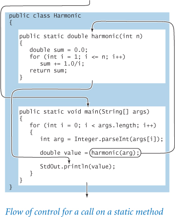
You can define static methods other than main() in a .java file by specifying a method signature, followed by a sequence of statements that constitute the method. We will consider the details shortly, but we begin with a simple example—Harmonic (PROGRAM 2.1.1)—that illustrates how methods affect control flow. It features a static method named harmonic() that takes an integer argument n and returns the nth harmonic number (see PROGRAM 1.3.5).
PROGRAM 2.1.1 is superior to our original implementation for computing harmonic numbers (PROGRAM 1.3.5) because it clearly separates the two primary tasks performed by the program: calculating harmonic numbers and interacting with the user. (For purposes of illustration, PROGRAM 2.1.1 takes several command-line arguments instead of just one.) Whenever you can clearly separate tasks within programs, you should do so.
Control flow
While Harmonic appeals to our familiarity with mathematical functions, we will examine it in detail so that you can think carefully about what a static method is and how it operates. Harmonic comprises two static methods: harmonic() and main(). Even though harmonic() appears first in the code, the first statement that Java executes is, as usual, the first statement in main(). The next few statements operate as usual, except that the code harmonic(arg), which is known as a call on the static method harmonic(), causes a transfer of control to the first line of code in harmonic(), each time that it is encountered. Moreover, Java initializes the parameter variable n in harmonic() to the value of arg in main() at the time of the call. Then, Java executes the statements in harmonic() as usual, until it reaches a return statement, which transfers control back to the statement in main() containing the call on harmonic(). Moreover, the method call harmonic(arg) produces a value—the value specified by the return statement, which is the value of the variable sum in harmonic() at the time that the return statement is executed. Java then assigns this return value to the variable value. The end result exactly matches our intuition: The first value assigned to value and printed is 1.0—the value computed by code in harmonic() when the parameter variable n is initialized to 1. The next value assigned to value and printed is 1.5—the value computed by harmonic() when n is initialized to 2. The same process is repeated for each command-line argument, transferring control back and forth between harmonic() and main().
Program 2.1.1 Harmonic numbers (revisited)
public class Harmonic
{
   public static double harmonic(int n)
   {
      double sum = 0.0;
      for (int i = 1; i <= n; i++)
         sum += 1.0/i;
      return sum;
   }

   public static void main(String[] args)
   {
      for (int i = 0; i < args.length; i++)
      {
         int arg = Integer.parseInt(args[i]);
         double value = harmonic(arg);
         StdOut.println(value);
      }
   }
}
sum | cumulated sum
 arg  | argument
value | return value
This program defines two static methods, one named harmonic() that has integer argument n and computes the nth harmonic numbers (see PROGRAM 1.3.5) and one named main(), which tests harmonic() with integer arguments specified on the command line.
% java Harmonic 1 2 4
1.0
1.5
2.083333333333333
% java Harmonic 10 100 1000 10000
2.9289682539682538
5.187377517639621
7.485470860550343
9.787606036044348
Function-call trace
One simple approach to following the control flow through function calls is to imagine that each function prints its name and argument value(s) when it is called and its return value just before returning, with indentation added on calls and subtracted on returns. The result enhances the process of tracing a program by printing the values of its variables, which we have been using since SECTION 1.2. The added indentation exposes the flow of the control, and helps us check that each function has the effect that we expect. Generally, adding calls on StdOut.println() to trace any program’s control flow in this way is a fine way to begin to understand what it is doing. If the return values match our expectations, we need not trace the function code in detail, saving us a substantial amount of work.
i = 0
arg = 1
harmonic(1)
   sum = 0.0
   sum = 1.0
   return 1.0
value = 1.0
i = 1
arg = 2
harmonic(2)
   sum = 0.0
   sum = 1.0
   sum = 1.5
   return 1.5
value = 1.5
i = 2
arg = 4
harmonic(4)
   sum = 0.0
   sum = 1.0
   sum = 1.5
   sum = 1.8333333333333333
   sum = 2.083333333333333
   return 2.083333333333333
value = 2.083333333333333
Function-call trace for java Harmonic 1 2 4
For the rest of this chapter, your programming will center on creating and using static methods, so it is worthwhile to consider in more detail their basic properties. Following that, we will study several examples of function implementations and applications.
Terminology
It is useful to draw a distinction between abstract concepts and Java mechanisms to implement them (the Java if statement implements the conditional, the while statement implements the loop, and so forth). Several concepts are rolled up in the idea of a mathematical function, and there are Java constructs corresponding to each, as summarized in the table at the top of the next page. While these formalisms have served mathematicians well for centuries (and have served programmers well for decades), we will refrain from considering in detail all of the implications of this correspondence and focus on those that will help you learn to program.
concept |
Java construct |
description |
function |
static method |
mapping |
input value |
argument |
input to function |
output value |
return value |
output from function |
formula |
method body |
function definition |
independent variable |
parameter variable |
symbolic placeholder for input value |
When we use a symbolic name in a formula that defines a mathematical function (such as f(x) = 1 + x + x2), the symbol x is a placeholder for some input value that will be substituted into the formula to determine the output value. In Java, we use a parameter variable as a symbolic placeholder and we refer to a particular input value where the function is to be evaluated as an argument.
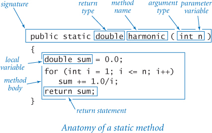
Static method definition
The first line of a static method definition, known as the signature, gives a name to the method and to each parameter variable. It also specifies the type of each parameter variable and the return type of the method. The signature consists of the keyword public; the keyword static; the return type; the method name; and a sequence of zero or more parameter variable types and names, separated by commas and enclosed in parentheses. We will discuss the meaning of the public keyword in the next section and the meaning of the static keyword in CHAPTER 3. (Technically, the signature in Java includes only the method name and parameter types, but we leave that distinction for experts.) Following the signature is the body of the method, enclosed in curly braces. The body consists of the kinds of statements we discussed in CHAPTER 1. It also can contain a return statement, which transfers control back to the point where the static method was called and returns the result of the computation or return value. The body may declare local variables, which are variables that are available only inside the method in which they are declared.
Function calls
As you have already seen, a static method call in Java is nothing more than the method name followed by its arguments, separated by commas and enclosed in parentheses, in precisely the same form as is customary for mathematical functions. As noted in SECTION 1.2, a method call is an expression, so you can use it to build up more complicated expressions. Similarly, an argument is an expression—Java evaluates the expression and passes the resulting value to the method. So, you can write code like Math.exp(-x*x/2) / Math.sqrt(2*Math.PI) and Java knows what you mean.

Multiple arguments
Like a mathematical function, a Java static method can take on more than one argument, and therefore can have more than one parameter variable. For example, the following static method computes the length of the hypotenuse of a right triangle with sides of length a and b:
public static double hypotenuse(double a, double b)
{  return Math.sqrt(a*a + b*b); }
Although the parameter variables are of the same type in this case, in general they can be of different types. The type and the name of each parameter variable are declared in the function signature, with the declarations for each variable separated by commas.
Multiple methods
You can define as many static methods as you want in a .java file. Each method has a body that consists of a sequence of statements enclosed in curly braces. These methods are independent and can appear in any order in the file. A static method can call any other static method in the same file or any static method in a Java library such as Math, as illustrated with this pair of methods:
public static double square(double a)
{  return a*a;  }

public static double hypotenuse(double a, double b)
{  return Math.sqrt(square(a) + square(b));  }
Also, as we see in the next section, a static method can call static methods in other .java files (provided they are accessible to Java). In SECTION 2.3, we consider the ramifications of the idea that a static method can even call itself.
Overloading
Static methods with different signatures are different static methods. For example, we often want to define the same operation for values of different numeric types, as in the following static methods for computing absolute values:
public static int abs(int x)
{
   if (x < 0) return -x;
   else       return  x;
}

public static double abs(double x)
{
   if (x < 0.0) return -x;
   else         return  x;
}
These are two different methods, but are sufficiently similar so as to justify using the same name (abs). Using the same name for two static methods whose signatures differ is known as overloading, and is a common practice in Java programming. For example, the Java Math library uses this approach to provide implementations of Math.abs(), Math.min(), and Math.max() for all primitive numeric types. Another common use of overloading is to define two different versions of a method: one that takes an argument and another that uses a default value for that argument.
Multiple return statements
You can put return statements in a method wherever you need them: control goes back to the calling program as soon as the first return statement is reached. This primality-testing function is an example of a function that is natural to define using multiple return statements:
public static boolean isPrime(int n)
{
   if (n < 2) return false;
   for (int i = 2; i <= n/i; i++)
      if (n % i == 0) return false;
   return true;
}
Even though there may be multiple return statements, any static method returns a single value each time it is invoked: the value following the first return statement encountered. Some programmers insist on having only one return per method, but we are not so strict in this book.
absolute value of an |
public static int abs(int x)
{
   if (x < 0) return -x;
   else       return x;
} |
absolute value of a |
public static double abs(double x)
{
   if (x < 0.0) return -x;
   else         return x;
} |
primality test |
public static boolean isPrime(int n)
{
   if (n < 2) return false;
   for (int i = 2; i <= n/i; i++)
      if (n % i == 0) return false;
   return true;
} |
hypotenuse of a right triangle |
public static double hypotenuse(double a, double b)
{ return Math.sqrt(a*a + b*b); } |
harmonic number |
public static double harmonic(int n)
{
   double sum = 0.0;
   for (int i = 1; i <= n; i++)
      sum += 1.0 / i;
   return sum;
} |
uniform random integer in [0, n ) |
public static int uniform(int n)
{ return (int) (Math.random() * n); } |
draw a triangle |
public static void drawTriangle(double x0, double y0,
                                double x1, double y1,
                                double x2, double y2 )
{
   StdDraw.line(x0, y0, x1, y1);
   StdDraw.line(x1, y1, x2, y2);
   StdDraw.line(x2, y2, x0, y0);
} |
Typical code for implementing functions (static methods) |
|
Single return value
A Java method provides only one return value to the caller, of the type declared in the method signature. This policy is not as restrictive as it might seem because Java data types can contain more information than the value of a single primitive type. For example, you will see later in this section that you can use arrays as return values.
Scope
The scope of a variable is the part of the program that can refer to that variable by name. The general rule in Java is that the scope of the variables declared in a block of statements is limited to the statements in that block. In particular, the scope of a variable declared in a static method is limited to that method’s body. Therefore, you cannot refer to a variable in one static method that is declared in another. If the method includes smaller blocks—for example, the body of an if or a for statement—the scope of any variables declared in one of those blocks is limited to just the statements within that block. Indeed, it is common practice to use the same variable names in independent blocks of code. When we do so, we are declaring different independent variables. For example, we have been following this practice when we use an index i in two different for loops in the same program. A guiding principle when designing software is that each variable should be declared so that its scope is as small as possible. One of the important reasons that we use static methods is that they ease debugging by limiting variable scope.

Side effects
In mathematics, a function maps one or more input values to some output value. In computer programming, many functions fit that same model: they accept one or more arguments, and their only purpose is to return a value. A pure function is a function that, given the same arguments, always returns the same value, without producing any observable side effects, such as consuming input, producing output, or otherwise changing the state of the system. The functions harmonic(), abs(), isPrime(), and hypotenuse() are examples of pure functions.
However, in computer programming it is also useful to define functions that do produce side effects. In fact, we often define functions whose only purpose is to produce side effects. In Java, a static method may use the keyword void as its return type, to indicate that it has no return value. An explicit return is not necessary in a void static method: control returns to the caller after Java executes the method’s last statement.
For example, the static method StdOut.println() has the side effect of printing the given argument to standard output (and has no return value). Similarly, the following static method has the side effect of drawing a triangle to standard drawing (and has no specified return value):
public static void drawTriangle(double x0, double y0,
                                double x1, double y1,
                                double x2, double y2)
{
   StdDraw.line(x0, y0, x1, y1);
   StdDraw.line(x1, y1, x2, y2);
   StdDraw.line(x2, y2, x0, y0);
}
It is generally poor style to write a static method that both produces side effects and returns a value. One notable exception arises in functions that read input. For ex-ample, StdIn.readInt() both returns a value (an integer) and produces a side effect (consuming one integer from standard input). In this book, we use void static methods for two primary purposes:
• For I/O, using StdIn, StdOut, StdDraw, and StdAudio
• To manipulate the contents of arrays
You have been using void static methods for output since main() in HelloWorld, and we will discuss their use with arrays later in this section. It is possible in Java to write methods that have other side effects, but we will avoid doing so until CHAPTER 3, where we do so in a specific manner supported by Java.
Implementing mathematical functions
Why not just use the methods that are defined within Java, such as Math.sqrt()? The answer to this question is that we do use such implementations when they are present. Unfortunately, there are an unlimited number of mathematical functions that we may wish to use and only a small set of functions in the library. When you encounter a mathematical function that is not in the library, you need to implement a corresponding static method.
As an example, we consider the kind of code required for a familiar and important application that is of interest to many high school and college students in the United States. In a recent year, more than 1 million students took a standard college entrance examination. Scores range from 400 (lowest) to 1600 (highest) on the multiple-choice parts of the test. These scores play a role in making important decisions: for example, student athletes are required to have a score of at least 820, and the minimum eligibility requirement for certain academic scholarships is 1500. What percentage of test takers are ineligible for athletics? What percentage are eligible for the scholarships?

Two functions from statistics enable us to compute accurate answers to these questions. The Gaussian (normal) probability density function is characterized by the familiar bell-shaped curve and defined by the formula . The Gaussian cumulative distribution function Φ(z) is defined to be the area under the curve defined by ϕ(x) above the x-axis and to the left of the vertical line x = z. These functions play an important role in science, engineering, and finance because they arise as accurate models throughout the natural world and because they are essential in understanding experimental error.
In particular, these functions are known to accurately describe the distribution of test scores in our example, as a function of the mean (average value of the scores) and the standard deviation (square root of the average of the sum of the squares of the differences between each score and the mean), which are published each year. Given the mean μ and the standard deviation σ of the test scores, the percentage of students with scores less than a given value z is closely approximated by the function Φ((z – μ)/σ). Static methods to calculate ϕ and Φ are not available in Java’s Math library, so we need to develop our own implementations.
Program 2.1.2 Gaussian functions
public class Gaussian
{  // Implement Gaussian (normal) distribution functions.
   public static double pdf(double x)
   {
      return Math.exp(-x*x/2) / Math.sqrt(2*Math.PI);
   }

   public static double cdf(double z)
   {
      if (z < -8.0) return 0.0;
      if (z > 8.0) return 1.0;
      double sum = 0.0;
      double term = z;
      for (int i = 3; sum != sum + term; i += 2)
      {
         sum = sum + term;
         term = term * z * z / i;
      }
      return 0.5 + pdf(z) * sum;
   }

   public static void main(String[] args)
   {
      double z     = Double.parseDouble(args[0]);
      double mu    = Double.parseDouble(args[1]);
      double sigma = Double.parseDouble(args[2]);
      StdOut.printf("%.3f
", cdf((z - mu) / sigma));
   }
}
 sum | cumulated sum
term | current term
This code implements the Gaussian probability density function (pdf) and Gaussian cumulative distribution function (cdf), which are not implemented in Java’s Math library. The pdf() implementation follows directly from its definition, and the cdf() implementation uses a Taylor series and also calls pdf() (see accompanying text and EXERCISE 1.3.38).
% java Gaussian 820 1019 209
0.171
% java Gaussian 1500 1019 209
0.989
% java Gaussian 1500 1025 231
0.980
Closed form
In the simplest situation, we have a closed-form mathematical formula defining our function in terms of functions that are implemented in the library. This situation is the case for ϕ—the Java Math library includes methods to compute the exponential and the square root functions (and a constant value for π), so a static method pdf() corresponding to the mathematical definition is easy to implement (see PROGRAM 2.1.2).
No closed form
Otherwise, we may need a more complicated algorithm to compute function values. This situation is the case for Φ—no closed-form expression exists for this function. Such algorithms sometimes follow immediately from Taylor series approximations, but developing reliably accurate implementations of mathematical functions is an art that needs to be addressed carefully, taking advantage of the knowledge built up in mathematics over the past several centuries. Many different approaches have been studied for evaluating Φ. For example, a Taylor series approximation to the ratio of Φ and ϕ turns out to be an effective basis for evaluating the function:
Φ(z) = 1/2 + ϕ(z) (z + z3 / 3 + z5 / (3·5) + z7 / (3·5·7) +. . .)
This formula readily translates to the Java code for the static method cdf() in PROGRAM 2.1.2. For small (respectively large) z, the value is extremely close to 0 (respectively 1), so the code directly returns 0 (respectively 1); otherwise, it uses the Taylor series to add terms until the sum converges.
Running Gaussian with the appropriate arguments on the command line tells us that about 17% of the test takers were ineligible for athletics and that only about 1% qualified for the scholarship. In a year when the mean was 1025 and the standard deviation 231, about 2% qualified for the scholarship.
Computing with mathematical functions of all kinds has always played a central role in science and engineering. In a great many applications, the functions that you need are expressed in terms of the functions in Java’s Math library, as we have just seen with pdf(), or in terms of Taylor series approximations that are easy to compute, as we have just seen with cdf(). Indeed, support for such computations has played a central role throughout the evolution of computing systems and programming languages. You will find many examples on the booksite and throughout this book.
Using static methods to organize code
Beyond evaluating mathematical functions, the process of calculating an output value on the basis of an input value is important as a general technique for organizing control flow in any computation. Doing so is a simple example of an extremely important principle that is a prime guiding force for any good programmer: whenever you can clearly separate tasks within programs, you should do so.
Functions are natural and universal for expressing computational tasks. Indeed, the “bird’s-eye view” of a Java program that we began with in SECTION 1.1 was equivalent to a function: we began by thinking of a Java program as a function that transforms command-line arguments into an output string. This view expresses itself at many different levels of computation. In particular, it is generally the case that a long program is more naturally expressed in terms of functions instead of as a sequence of Java assignment, conditional, and loop statements. With the ability to define functions, we can better organize our programs by defining functions within them when appropriate.
For example, Coupon (PROGRAM 2.1.3) is a version of CouponCollector (PROGRAM 1.4.2) that better separates the individual components of the computation. If you study PROGRAM 1.4.2, you will identify three separate tasks:
• Given n, compute a random coupon value.
• Given n, do the coupon collection experiment.
• Get n from the command line, and then compute and print the result.
Coupon rearranges the code in CouponCollector to reflect the reality that these three functions underlie the computation. With this organization, we could change getCoupon() (for example, we might want to draw the random numbers from a different distribution) or main() (for example, we might want to take multiple inputs or run multiple experiments) without worrying about the effect of any changes in collectCoupons().
Using static methods isolates the implementation of each component of the collection experiment from others, or encapsulates them. Typically, programs have many independent components, which magnifies the benefits of separating them into different static methods. We will discuss these benefits in further detail after we have seen several other examples, but you certainly can appreciate that it is better to express a computation in a program by breaking it up into functions, just as it is better to express an idea in an essay by breaking it up into paragraphs. Whenever you can clearly separate tasks within programs, you should do so.
Program 2.1.3 Coupon collector (revisited)
public class Coupon
{
   public static int getCoupon(int n)
   {  // Return a random integer between 0 and n-1.
      return (int) (Math.random() * n);
   }

   public static int collectCoupons(int n)
   {  // Collect coupons until getting one of each value
      // and return the number of coupons collected.
      boolean[] isCollected = new boolean[n];
      int count = 0, distinct = 0;
      while (distinct < n)
      {
         int r = getCoupon(n);
         count++;
         if (!isCollected[r])
            distinct++;
         isCollected[r] = true;
      }
      return count;
   }

   public static void main(String[] args)
   {  // Collect n different coupons.
      int n = Integer.parseInt(args[0]);
      int count = collectCoupons(n);
      StdOut.println(count);
   }
}
      n       | # coupon values (0 to n-1)
isCollected[i]| has coupon i been collected?
     count    | # coupons collected
   distinct   | # distinct coupons collected
      r       | random coupon
This version of PROGRAM 1.4.2 illustrates the style of encapsulating computations in static methods. This code has the same effect as CouponCollector, but better separates the code into its three constituent pieces: generating a random integer between 0 and n-1, running a coupon collection experiment, and managing the I/O.
% java Coupon 1000
6522
% java Coupon 1000
6481
% java Coupon 10000
105798
% java Coupon 1000000
12783771
Passing arguments and returning values
Next, we examine the specifics of Java’s mechanisms for passing arguments to and returning values from functions. These mechanisms are conceptually very simple, but it is worthwhile to take the time to understand them fully, as the effects are actually profound. Understanding argument-passing and return-value mechanisms is key to learning any new programming language.
Pass by value
You can use parameter variables anywhere in the code in the body of the function in the same way you use local variables. The only difference between a parameter variable and a local variable is that Java evaluates the argument provided by the calling code and initializes the parameter variable with the resulting value. This approach is known as pass by value. The method works with the value of its arguments, not the arguments themselves. One consequence of this approach is that changing the value of a parameter variable within a static method has no effect on the calling code. (For clarity, we do not change parameter variables in the code in this book.) An alternative approach known as pass by reference, where the method works directly with the calling code’s arguments, is favored in some programming environments.
A static method can take an array as an argument or return an array to the caller. This capability is a special case of Java’s object orientation, which is the subject of CHAPTER 3. We consider it in the present context because the basic mechanisms are easy to understand and to use, leading us to compact solutions to a number of problems that naturally arise when we use arrays to help us process large amounts of data.
Arrays as arguments
When a static method takes an array as an argument, it implements a function that operates on an arbitrary number of values of the same type. For example, the following static method computes the mean (average) of an array of double values:
public static double mean(double[] a)
{
   double sum = 0.0;
   for (int i = 0; i < a.length; i++)
      sum += a[i];
   return sum / a.length;
}
We have been using arrays as arguments since our first program. The code
public static void main(String[] args)
defines main() as a static method that takes an array of strings as an argument and returns nothing. By convention, the Java system collects the strings that you type after the program name in the java command into an array and calls main() with that array as argument. (Most programmers use the name args for the parameter variable, even though any name at all would do.) Within main(), we can manipulate that array just like any other array.
Side effects with arrays
It is often the case that the purpose of a static method that takes an array as argument is to produce a side effect (change values of array elements). A prototypical example of such a method is one that exchanges the values at two given indices in a given array. We can adapt the code that we examined at the beginning of SECTION 1.4:
public static void exchange(String[] a, int i, int j)
{
   String temp = a[i];
   a[i] = a[j];
   a[j] = temp;
}
This implementation stems naturally from the Java array representation. The parameter variable in exchange() is a reference to the array, not a copy of the array values: when you pass an array as an argument to a method, the method has an opportunity to reassign values to the elements in that array. A second prototypical example of a static method that takes an array argument and produces side effects is one that randomly shuffles the values in the array, using this version of the algorithm that we examined in SECTION 1.4 (and the exchange() and uniform() methods considered earlier in this section):
public static void shuffle(String[] a)
{
   int n = a.length;
   for (int i = 0; i < n; i++)
      exchange(a, i, i + uniform(n-i));
}
find the maximum of the array values |
public static double max(double[] a)
{
   double max = Double.NEGATIVE_INFINITY;
   for (int i = 0; i < a.length; i++)
      if (a[i] > max) max = a[i];
   return max;
} |
dot product |
public static double dot(double[] a, double[] b)
{
   double sum = 0.0;
   for (int i = 0; i < a.length; i++)
      sum += a[i] * b[i];
   return sum;
} |
exchange the values of two elements in an array |
public static void exchange(String[] a, int i, int j)
{
   String temp = a[i];
   a[i] = a[j];
   a[j] = temp;
} |
print a one-dimensional array (and its length) |
public static void print(double[] a)
{
   StdOut.println(a.length);
   for (int i = 0; i < a.length; i++)
      StdOut.println(a[i]);
} |
read a 2D array of |
public static double[][] readDouble2D()
{
   int m = StdIn.readInt();
   int n = StdIn.readInt();
   double[][] a = new double[m][n];
   for (int i = 0; i < m; i++)
      for (int j = 0; j < n; j++)
         a[i][j] = StdIn.readDouble();
   return a;
} |
Typical code for implementing functions with array arguments or return values |
|
Similarly, we will consider in SECTION 4.2 methods that sort an array (rearrange its values so that they are in order). All of these examples highlight the basic fact that the mechanism for passing arrays in Java is call by value with respect to the array reference but call by reference with respect to the array elements. Unlike primitive-type arguments, the changes that a method makes to the elements of an array are reflected in the client program. A method that takes an array as its argument cannot change the array itself—the memory location, length, and type of the array are the same as they were when the array was created—but a method can assign different values to the elements in the array.
Arrays as return values
A method that sorts, shuffles, or otherwise modifies an array taken as an argument does not have to return a reference to that array, because it is changing the elements of a client array, not a copy. But there are many situations where it is useful for a static method to provide an array as a return value. Chief among these are static methods that create arrays for the purpose of returning multiple values of the same type to a client. For example, the following static method creates and returns an array of the kind used by StdAudio (see PROGRAM 1.5.7): it contains values sampled from a sine wave of a given frequency (in hertz) and duration (in seconds), sampled at the standard 44,100 samples per second.
public static double[] tone(double hz, double t)
{
   int SAMPLING_RATE = 44100;
   int n = (int) (SAMPLING_RATE * t);
   double[] a = new double[n+1];
   for (int i = 0; i <= n; i++)
      a[i] = Math.sin(2 * Math.PI * i * hz / SAMPLING_RATE);
   return a;
}
In this code, the length of the array returned depends on the duration: if the given duration is t, the length of the array is about 44100*t. With static methods like this one, we can write code that treats a sound wave as a single entity (an array containing sampled values), as we will see next in PROGRAM 2.1.4.
Example: superposition of sound waves
As discussed in SECTION 1.5, the simple audio model that we studied there needs to be embellished to create sound that resembles the sound produced by a musical instrument. Many different embellishments are possible; with static methods we can systematically apply them to produce sound waves that are far more complicated than the simple sine waves that we produced in SECTION 1.5. As an illustration of the effective use of static methods to solve an interesting computational problem, we consider a program that has essentially the same functionality as PlayThatTune (PROGRAM 1.5.7), but adds harmonic tones one octave above and one octave below each note to produce a more realistic sound.
Chords and harmonics
Notes like concert A have a pure sound that is not very musical, because the sounds that you are accustomed to hearing have many other components. The sound from the guitar string echoes off the wooden part of the instrument, the walls of the room that you are in, and so forth. You may think of such effects as modifying the basic sine wave. For example, most musical instruments produce harmonics (the same note in different octaves and not as loud), or you might play chords (multiple notes at the same time). To combine multiple sounds, we use superposition: simply add the waves together and rescale to make sure that all values stay between –1 and +1. As it turns out, when we superpose sine waves of different frequencies in this way, we can get arbitrarily complicated waves. Indeed, one of the triumphs of 19th-century mathematics was the development of the idea that any smooth periodic function can be expressed as a sum of sine and cosine waves, known as a Fourier series. This mathematical idea corresponds to the notion that we can create a large range of sounds with musical instruments or our vocal cords and that all sound consists of a composition of various oscillating curves. Any sound corresponds to a curve and any curve corresponds to a sound, and we can create arbitrarily complex curves with superposition.

Weighted superposition
Since we represent sound waves by arrays of numbers that represent their values at the same sample points, superposition is simple to implement: we add together the values at each sample point to produce the combined result and then rescale. For greater control, we specify a relative weight for each of the two waves to be added, with the property that the weights are positive and sum to 1. For example, if we want the first sound to have three times the effect of the second, we would assign the first a weight of 0.75 and the second a weight of 0.25. Now, if one wave is in an array a[] with relative weight awt and the other is in an array b[] with relative weight bwt, we compute their weighted sum with the following code:
double[] c = new double[a.length];
for (int i = 0; i < a.length; i++)
  c[i] = a[i]*awt + b[i]*bwt;
The conditions that the weights are positive and sum to 1 ensure that this operation preserves our convention of keeping the values of all of our waves between –1 and +1.

Program 2.1.4 Play that tune (revisited)
public class PlayThatTuneDeluxe
{
   public static double[] superpose(double[] a, double[] b,
                                    double awt, double bwt)
   {  // Weighted superposition of a and b.
      double[] c = new double[a.length];
      for (int i = 0; i < a.length; i++)
         c[i] = a[i]*awt + b[i]*bwt;
      return c;
   }

   public static double[] tone(double hz, double t)
   {  /* see text */ }

   public static double[] note(int pitch, double t)
   {  // Play note of given pitch, with harmonics.
      double hz = 440.0 * Math.pow(2, pitch / 12.0);
      double[] a = tone(hz, t);
      double[] hi = tone(2*hz, t);
      double[] lo = tone(hz/2, t);
      double[] h = superpose(hi, lo, 0.5, 0.5);
      return superpose(a, h, 0.5, 0.5);
   }

   public static void main(String[] args)
   {  // Read and play a tune, with harmonics.
      while (!StdIn.isEmpty())
      {  // Read and play a note, with harmonics.
         int pitch = StdIn.readInt();
         double duration = StdIn.readDouble();
         double[] a = note(pitch, duration);
         StdAudio.play(a);
      }
   }
}
  hz | frequency
 a[] | pure tone
hi[] | upper harmonic
lo[] | lower harmonic
 h[] | tone with harmonics
This code embellishes the sounds produced by PROGRAM 1.5.7 by using static methods to create harmonics, which results in a more realistic sound than the pure tone.
% more elise.txt
7 0.25
6 0.25
7 0.25
6 0.25
...

PROGRAM 2.1.4 is an implementation that applies these concepts to produce a more realistic sound than that produced by PROGRAM 1.5.7. To do so, it makes use of functions to divide the computation into four parts:
• Given a frequency and duration, create a pure tone.
• Given two sound waves and relative weights, superpose them.
• Given a pitch and duration, create a note with harmonics.
• Read and play a sequence of pitch/duration pairs from standard input.
These tasks are each amenable to implementation as a function, with all of the functions then depending on one another. Each function is well defined and straightforward to implement. All of them (and StdAudio) represent sound as a sequence of floating-point numbers kept in an array, corresponding to sampling a sound wave at 44,100 samples per second.
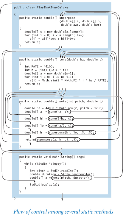
Up to this point, the use of functions has been somewhat of a notational convenience. For example, the control flow in PROGRAM 2.1.1–2.1.3 is simple—each function is called in just one place in the code. By contrast, PlayThatTuneDeluxe (PROGRAM 2.1.4) is a convincing example of the effectiveness of defining functions to organize a computation because the functions are each called multiple times. For example, the function note() calls the function tone() three times and the function superpose() twice. Without functions methods, we would need multiple copies of the code in tone() and superpose(); with functions, we can deal directly with concepts close to the application. Like loops, functions have a simple but profound effect: one sequence of statements (those in the method definition) is executed multiple times during the execution of our program—once for each time the function is called in the control flow in main().
Functions (static methods) are important because they give us the ability to extend the Java language within a program. Having implemented and debugged functions such as harmonic(), pdf(), cdf(), mean(), abs(), exchange(), shuffle(), isPrime(), uniform(), superpose(), note(), and tone(), we can use them almost as if they were built into Java. The flexibility to do so opens up a whole new world of programming. Before, you were safe in thinking about a Java program as a sequence of statements. Now you need to think of a Java program as a set of static methods that can call one another. The statement-to-statement control flow to which you have been accustomed is still present within static methods, but programs have a higher-level control flow defined by static method calls and returns. This ability enables you to think in terms of operations called for by the application, not just the simple arithmetic operations on primitive types that are built into Java.
Whenever you can clearly separate tasks within programs, you should do so. The examples in this section (and the programs throughout the rest of the book) clearly illustrate the benefits of adhering to this maxim. With static methods, we can
• Divide a long sequence of statements into independent parts.
• Reuse code without having to copy it.
• Work with higher-level concepts (such as sound waves).
This produces code that is easier to understand, maintain, and debug than a long program composed solely of Java assignment, conditional, and loop statements. In the next section, we discuss the idea of using static methods defined in other programs, which again takes us to another level of programming.
A. As usual, the best way to answer a question like this is to try it yourself and see what happens. Here is the result of omitting the static modifier from harmonic() in Harmonic:
Harmonic.java:15: error: non-static method harmonic(int)
cannot be referenced from a static context
         double value = harmonic(arg);
                        ^
1 error
Non-static methods are different from static methods. You will learn about the former in CHAPTER 3.
Q. What happens if I write code after a return statement?
A. Once a return statement is reached, control immediately returns to the caller, so any code after a return statement is useless. Java identifies this situation as a compile-time error, reporting unreachable code.
Q. What happens if I do not include a return statement?
A. There is no problem, if the return type is void. In this case, control will return to the caller after the last statement. When the return type is not void, Java will report a missing return statement compile-time error if there is any path through the code that does not end in a return statement.
Q. Why do I need to use the return type void? Why not just omit the return type?
A. Java requires it; we have to include it. Second-guessing a decision made by a programming-language designer is the first step on the road to becoming one.
Q. Can I return from a void function by using return? If so, which return value should I use?
A. Yes. Use the statement return; with no return value.
Q. This issue with side effects and arrays passed as arguments is confusing. Is it really all that important?
A. Yes. Properly controlling side effects is one of a programmer’s most important tasks in large systems. Taking the time to be sure that you understand the difference between passing a value (when arguments are of a primitive type) and passing a reference (when arguments are arrays) will certainly be worthwhile. The very same mechanism is used for all other types of data, as you will learn in CHAPTER 3.
Q. So why not just eliminate the possibility of side effects by making all arguments pass by value, including arrays?
A. Think of a huge array with, say, millions of elements. Does it make sense to copy all of those values for a static method that is going to exchange just two of them? For this reason, most programming languages support passing an array to a function without creating a copy of the array elements—Matlab is a notable exception.
Q. In which order does Java evaluate method calls?
A. Regardless of operator precedence or associativity, Java evaluates subexpressions (including method calls) and argument lists from left to right. For example, when evaluating the expression
f1() + f2() * f3(f4(), f5())
Java calls the methods in the order f1(), f2(), f4(), f5(), and f3(). This is most relevant for methods that produce side effects. As a matter of style, we avoid writing code that depends on the order of evaluation.
Exercises
2.1.1 Write a static method max3() that takes three int arguments and returns the value of the largest one. Add an overloaded function that does the same thing with three double values.
2.1.2 Write a static method odd() that takes three boolean arguments and returns true if an odd number of the argument values are true, and false otherwise.
2.1.3 Write a static method majority() that takes three boolean arguments and returns true if at least two of the argument values are true, and false otherwise. Do not use an if statement.
2.1.4 Write a static method eq() that takes two int arrays as arguments and returns true if the arrays have the same length and all corresponding pairs of of elements are equal, and false otherwise.
2.1.5 Write a static method areTriangular() that takes three double arguments and returns true if they could be the sides of a triangle (none of them is greater than or equal to the sum of the other two). See EXERCISE 1.2.15.
2.1.6 Write a static method sigmoid() that takes a double argument x and returns the double value obtained from the formula 1 / (1 + e–x).
2.1.7 Write a static method sqrt() that takes a double argument and returns the square root of that number. Use Newton’s method (see PROGRAM 1.3.6) to compute the result.
2.1.8 Give the function-call trace for java Harmonic 3 5
2.1.9 Write a static method lg() that takes a double argument n and returns the base-2 logarithm of n. You may use Java’s Math library.
2.1.10 Write a static method lg() that takes an int argument n and returns the largest integer not larger than the base-2 logarithm of n. Do not use the Math library.
2.1.11 Write a static method signum() that takes an int argument n and returns -1 if n is less than 0, 0 if n is equal to 0, and +1 if n is greater than 0.
2.1.12 Consider the static method duplicate() below.
public static String duplicate(String s)
{
   String t = s + s;
   return t;
}
What does the following code fragment do?
String s = "Hello";
s = duplicate(s);
String t = "Bye";
t = duplicate(duplicate(duplicate(t)));
StdOut.println(s + t);
2.1.13 Consider the static method cube() below.
public static void cube(int i)
{
   i = i * i * i;
}
How many times is the following for loop iterated?
for (int i = 0; i < 1000; i++)
   cube(i);
Answer: Just 1,000 times. A call to cube() has no effect on the client code. It changes the value of its local parameter variable i, but that change has no effect on the i in the for loop, which is a different variable. If you replace the call to cube(i) with the statement i = i * i * i; (maybe that was what you were thinking), then the loop is iterated five times, with i taking on the values 0, 1, 2, 9, and 730 at the beginning of the five iterations.
2.1.14 The following checksum formula is widely used by banks and credit card companies to validate legal account numbers:
d0 + f(d1) + d2 + f(d3) + d4 + f(d5) + ... = 0 (mod 10)
The di are the decimal digits of the account number and f (d) is the sum of the decimal digits of 2d (for example, f (7) = 5 because 2 × 7 = 14 and 1 + 4 = 5). For example, 17,327 is valid because 1 + 5 + 3 + 4 + 7 = 20, which is a multiple of 10. Implement the function f and write a program to take a 10-digit integer as a command-line argument and print a valid 11-digit number with the given integer as its first 10 digits and the checksum as the last digit.
2.1.15 Given two stars with angles of declination and right ascension (d1, a1) and (d2, a2), the angle they subtend is given by the formula
2 arcsin((sin2(d/2) + cos (d1)cos(d2)sin2(a/2))1/2)
where a1 and a2 are angles between –180 and 180 degrees, d1 and d2 are angles between –90 and 90 degrees, a = a2 – a1, and d = d2 – d1. Write a program to take the declination and right ascension of two stars as command-line arguments and print the angle they subtend. Hint: Be careful about converting from degrees to radians.
2.1.16 Write a static method scale() that takes a double array as its argument and has the side effect of scaling the array so that each element is between 0 and 1 (by subtracting the minimum value from each element and then dividing each element by the difference between the minimum and maximum values). Use the max() method defined in the table in the text, and write and use a matching min() method.
2.1.17 Write a static method reverse() that takes an array of strings as its argument and returns a new array with the strings in reverse order. (Do not change the order of the strings in the argument array.) Write a static method reverseInplace() that takes an array of strings as its argument and produces the side effect of reversing the order of the strings in the argument array.
2.1.18 Write a static method readBoolean2D() that reads a two-dimensional boolean matrix (with dimensions) from standard input and returns the resulting two-dimensional array.
2.1.19 Write a static method histogram() that takes an int array a[] and an integer m as arguments and returns an array of length m whose ith element is the number of times the integer i appeared in a[]. Assuming the values in a[] are all between 0 and m-1, the sum of the values in the returned array should equal a.length.
2.1.20 Assemble code fragments in this section and in SECTION 1.4 to develop a program that takes an integer command-line argument n and prints n five-card hands, separated by blank lines, drawn from a randomly shuffled card deck, one card per line using card names like Ace of Clubs.
2.1.21 Write a static method multiply() that takes two square matrices of the same dimension as arguments and produces their product (another square matrix of that same dimension). Extra credit: Make your program work whenever the number of columns in the first matrix is equal to the number of rows in the second matrix.
2.1.22 Write a static method any() that takes a boolean array as its argument and returns true if any of the elements in the array is true, and false otherwise. Write a static method all() that takes an array of boolean values as its argument and returns true if all of the elements in the array are true, and false otherwise.
2.1.23 Develop a version of getCoupon() that better models the situation when one of the coupons is rare: choose one of the n values at random, return that value with probability 1 /(1,000n), and return all other values with equal probability. Extra credit: How does this change affect the expected number of coupons that need to be collected in the coupon collector problem?
2.1.24 Modify PlayThatTune to add harmonics two octaves away from each note, with half the weight of the one-octave harmonics.
Creative Exercises
2.1.25 Birthday problem. Develop a class with appropriate static methods for studying the birthday problem (see EXERCISE 1.4.38).
2.1.26 Euler’s totient function. Euler’s totient function is an important function in number theory: φ(n) is defined as the number of positive integers less than or equal to n that are relatively prime with n (no factors in common with n other than 1). Write a class with a static method that takes an integer argument n and returns φ(n), and a main() that takes an integer command-line argument, calls the method with that argument, and prints the resulting value.
2.1.27 Harmonic numbers. Write a program Harmonic that contains three static methods harmoinc(), harmoincSmall(), and harmonicLarge() for computing the harmonic numbers. The harmonicSmall() method should just compute the sum (as in PROGRAM 1.3.5), the harmonicLarge() method should use the approximation Hn = loge(n) + γ + 1/(2n) – 1/(12n2) + 1/(120n4) (the number γ = 0.577215664901532... is known as Euler’s constant), and the harmonic() method should call harmonicSmall() for n < 100 and harmonicLarge() otherwise.
2.1.28 Black–Scholes option valuation. The Black–Scholes formula supplies the theoretical value of a European call option on a stock that pays no dividends, given the current stock price s, the exercise price x, the continuously compounded risk-free interest rate r, the volatility σ, and the time (in years) to maturity t. The Black–Scholes value is given by the formula s Φ(a) – x e–r t Φ(b), where Φ(z) is the Gaussian cumulative distribution function, , and . Write a program that takes s, r, σ, and t from the command line and prints the Black–Scholes value.
2.1.29 Fourier spikes. Write a program that takes a command-line argument n and plots the function
(cos(t) + cos(2 t) + cos(3 t) + ... + cos(n t)) / n
for 500 equally spaced samples of t from –10 to 10 (in radians). Run your program for n = 5 and n = 500. Note: You will observe that the sum converges to a spike (0 everywhere except a single value). This property is the basis for a proof that any smooth function can be expressed as a sum of sinusoids.
2.1.30 Calendar. Write a program Calendar that takes two integer command-line arguments m and y and prints the monthly calendar for month m of year y, as in this example:
% java Calendar 2 2009
February 2009
 S  M Tu  W Th  F  S
 1  2  3  4  5  6  7
 8  9 10 11 12 13 14
15 16 17 18 19 20 21
22 23 24 25 26 27 28
Hint: See LeapYear (PROGRAM 1.2.4) and EXERCISE 1.2.29.
2.1.31 Horner’s method. Write a class Horner with a method evaluate() that takes a floating-point number x and array p[] as arguments and returns the result of evaluating the polynomial whose coefficients are the elements in p[] at x:
p(x) = p0 + p1x1 + p2 x2 + ... + pn–2 xn–2 + pn–1 xn–1
Use Horner’s method, an efficient way to perform the computations that is suggested by the following parenthesization:
p(x) = p0+ x (p1 + x (p2 + ... + x (pn–2 +x pn–1)) . . .)
Write a test client with a static method exp() that uses evaluate() to compute an approximation to ex, using the first n terms of the Taylor series expansion ex = 1 + x + x2/2! + x3/3! + .... Your client should take a command-line argument x and compare your result against that computed by Math.exp(x).
2.1.32 Chords. Develop a version of PlayThatTune that can handle songs with chords (including harmonics). Develop an input format that allows you to specify different durations for each chord and different amplitude weights for each note within a chord. Create test files that exercise your program with various chords and harmonics, and create a version of Für Elise that uses them.
2.1.33 Benford’s law. The American astronomer Simon Newcomb observed a quirk in a book that compiled logarithm tables: the beginning pages were much grubbier than the ending pages. He suspected that scientists performed more computations with numbers starting with 1 than with 8 or 9, and postulated that, under general circumstances, the leading digit is much more likely to be 1 (roughly 30%) than the digit 9 (less than 4%). This phenomenon is known as Benford’s law and is now often used as a statistical test. For example, IRS forensic accountants rely on it to discover tax fraud. Write a program that reads in a sequence of integers from standard input and tabulates the number of times each of the digits 1–9 is the leading digit, breaking the computation into a set of appropriate static methods. Use your program to test the law on some tables of information from your computer or from the web. Then, write a program to foil the IRS by generating random amounts from $1.00 to $1,000.00 with the same distribution that you observed.
2.1.34 Binomial distribution. Write a function
public static double binomial(int n, int k, double p)
to compute the probability of obtaining exactly k heads in n biased coin flips (heads with probability p) using the formula
f (n, k, p) = pk(1–p)n–k n! / (k!(n–k)!)
Hint: To stave off overflow, compute x = ln f (n, k, p) and then return ex. In main(), take n and p from the command line and check that the sum over all values of k between 0 and n is (approximately) 1. Also, compare every value computed with the normal approximation
f (n, k, p) ≈ ϕ(np, np(1–p))
(see EXERCISE 2.2.1).
2.1.35 Coupon collecting from a binomial distribution. Develop a version of getCoupon() that uses binomial() from the previous exercise to return coupon values according to the binomial distribution with p = 1/2. Hint: Generate a uniformly random number x between 0 and 1, then return the smallest value of k for which the sum of f (n, j, p) for all j < k exceeds x. Extra credit: Develop a hypothesis for describing the behavior of the coupon collector function under this assumption.
2.1.36 Postal bar codes. The barcode used by the U.S. Postal System to route mail is defined as follows: Each decimal digit in the ZIP code is encoded using a sequence of three half-height and two full-height bars. The barcode starts and ends with a full-height bar (the guard rail) and includes a checksum digit (after the five-digit ZIP code or ZIP+4), computed by summing up the original digits modulo 10. Implement the following functions
• Draw a half-height or full-height bar on StdDraw.
• Given a digit, draw its sequence of bars.
• Compute the checksum digit.
Also implement a test client that reads in a five- (or nine-) digit ZIP code as the command-line argument and draws the corresponding postal bar code.

2.2 Libraries and Clients
Each program that you have written so far consists of Java code that resides in a single .java file. For large programs, keeping all the code in a single file in this way is restrictive and unnecessary. Fortunately, it is very easy in Java to refer to a method in one file that is defined in another. This ability has two important consequences on our style of programming.
First, it enables code reuse. One program can make use of code that is already written and debugged, not by copying the code, but just by referring to it. This ability to define code that can be reused is an essential part of modern programming. It amounts to extending Java—you can define and use your own operations on data.
Second, it enables modular programming. You can not only divide a program up into static methods, as just described in SECTION 2.1, but also keep those methods in different files, grouped together according to the needs of the application. Modular programming is important because it allows us to independently develop, compile, and debug parts of big programs one piece at a time, leaving each finished piece in its own file for later use without having to worry about its details again. We develop libraries of static methods for use by any other program, keeping each library in its own file and using its methods in any other program. Java’s Math library and our Std* libraries for input/output are examples that you have already used. More importantly, you will soon see that it is very easy to define libraries of your own. The ability to define libraries and then to use them in multiple programs is a critical aspect of our ability to build programs to address complex tasks.
Having just moved in SECTION 2.1 from thinking of a Java program as a sequence of statements to thinking of a Java program as a class comprising a set of static methods (one of which is main()), you will be ready after this section to think of a Java program as a set of classes, each of which is an independent module consisting of a set of methods. Since each method can call a method in another class, all of your code can interact as a network of methods that call one another, grouped together in classes. With this capability, you can start to think about managing complexity when programming by breaking up programming tasks into classes that can be implemented and tested independently.
Using static methods in other programs
To refer to a static method in one class that is defined in another, we use the same mechanism that we have been using to invoke methods such as Math.sqrt() and StdOut.println():
• Make both classes accessible to Java (for example, by putting them both in the same directory in your computer).
• To call a method, prepend its class name and a period separator.
For example, we might wish to write a simple client SAT.java that takes an SAT score z from the command line and prints the percentage of students scoring less than z in a given year (in which the mean score was 1,019 and its standard deviation was 209). To get the job done, SAT.java needs to compute Φ((z–1,019) / 209), a task perfectly suited for the cdf() method in Gaussian.java (PROGRAM 2.1.2). All that we need to do is to keep Gaussian.java in the same directory as SAT.java and prepend the class name when calling cdf(). Moreover, any other class in that directory can make use of the static methods defined in Gaussian, by calling Gaussian.pdf() or Gaussian.cdf(). The Math library is always accessible in Java, so any class can call Math.sqrt() and Math.exp(), as usual. The files Gaussian.java, SAT.java, and Math.java implement Java classes that interact with one another: SAT calls a method in Gaussian, which calls another method in Gaussian, which then calls two methods in Math.

The potential effect of programming by defining multiple files, each an independent class with multiple methods, is another profound change in our programming style. Generally, we refer to this approach as modular programming. We independently develop and debug methods for an application and then utilize them at any later time. In this section, we will consider numerous illustrative examples to help you get used to the idea. However, there are several details about the process that we need to discuss before considering more examples.
The public keyword
We have been identifying every static method as public since HelloWorld. This modifier identifies the method as available for use by any other program with access to the file. You can also identify methods as private (and there are a few other categories), but you have no reason to do so at this point. We will discuss various options in SECTION 3.3.
Each module is a class
We use the term module to refer to all the code that we keep in a single file. In Java, by convention, each module is a Java class that is kept in a file with the same name of the class but has a .java extension. In this chapter, each class is merely a set of static methods (one of which is main()). You will learn much more about the general structure of the Java class in CHAPTER 3.
The .class file
When you compile the program (by typing javac followed by the class name), the Java compiler makes a file with the class name followed by a .class extension that has the code of your program in a language more suited to your computer. If you have a .class file, you can use the module’s methods in another program even without having the source code in the corresponding .java file (but you are on your own if you discover a bug!).
Compile when necessary
When you compile a program, Java typically compiles everything that needs to be compiled in order to run that program. If you call Gaussian.cdf() in SAT, then, when you type javac SAT.java, the compiler will also check whether you modified Gaussian.java since the last time it was compiled (by checking the time it was last changed against the time Gaussian.class was created). If so, it will also compile Gaussian.java! If you think about this approach, you will agree that it is actually quite helpful. After all, if you find a bug in Gaussian.java (and fix it), you want all the classes that call methods in Gaussian to use the new version.
Multiple main() methods
Another subtle point is to note that more than one class might have a main() method. In our example, both SAT and Gaussian have their own main() method. If you recall the rule for executing a program, you will see that there is no confusion: when you type java followed by a class name, Java transfers control to the machine code corresponding to the main() method defined in that class. Typically, we include a main() method in every class, to test and debug its methods. When we want to run SAT, we type java SAT; when we want to debug Gaussian, we type java Gaussian (with appropriate command-line arguments).
If you think of each program that you write as something that you might want to make use of later, you will soon find yourself with all sorts of useful tools. Modular programming allows us to view every solution to a computational problem that we may develop as adding value to our computational environment.
For example, suppose that you need to evaluate Φ for some future application. Why not just cut and paste the code that implements cdf() from Gaussian? That would work, but would leave you with two copies of the code, making it more difficult to maintain. If you later want to fix or improve this code, you would need to do so in both copies. Instead, you can just call Gaussian.cdf(). Our implementations and uses of our methods are soon going to proliferate, so having just one copy of each is a worthy goal.
From this point forward, you should write every program by identifying a reasonable way to divide the computation into separate parts of a manageable size and implementing each part as if someone will want to use it later. Most frequently, that someone will be you, and you will have yourself to thank for saving the effort of rewriting and re-debugging code.
Libraries
We refer to a module whose methods are primarily intended for use by many other programs as a library. One of the most important characteristics of programming in Java is that thousands of libraries have been predefined for your use. We reveal information about those that might be of interest to you throughout the book, but we will postpone a detailed discussion of the scope of Java libraries, because many of them are designed for use by experienced programmers. Instead, we focus in this chapter on the even more important idea that we can build user-defined libraries, which are nothing more than classes that contain a set of related methods for use by other programs. No Java library can contain all the methods that we might need for a given computation, so this ability to create our own library of methods is a crucial step in addressing complex programming applications.

Clients
We use the term client to refer to a program that calls a given library method. When a class contains a method that is a client of a method in another class, we say that the first class is a client of the second class. In our example, SAT is a client of Gaussian. A given class might have multiple clients. For example, all of the programs that you have written that call Math.sqrt() or Math.random() are clients of Math.
APIs
Programmers normally think in terms of a contract between the client and the implementation that is a clear specification of what the method is to do. When you are writing both clients and implementations, you are making contracts with yourself, which by itself is helpful because it provides extra help in debugging. More important, this approach enables code reuse. You have been able to write programs that are clients of Std* and Math and other built-in Java classes because of an informal contract (an English-language description of what they are supposed to do) along with a precise specification of the signatures of the methods that are available for use. Collectively, this information is known as an application programming interface (API). This same mechanism is effective for user-defined libraries. The API allows any client to use the library without having to examine the code in the implementation, as you have been doing for Math and Std*. The guiding principle in API design is to provide to clients the methods they need and no others. An API with a huge number of methods may be a burden to implement; an API that is lacking important methods may be unnecessarily inconvenient for clients.
Implementations
We use the term implementation to describe the Java code that implements the methods in an API, kept by convention in a file with the library name and a .java extension. Every Java program is an implementation of some API, and no API is of any use without some implementation. Our goal when developing an implementation is to honor the terms of the contract. Often, there are many ways to do so, and separating client code from implementation code gives us the freedom to substitute new and improved implementations.
For example, consider the Gaussian distribution functions. These do not appear in Java’s Math library but are important in applications, so it is worthwhile for us to put them in a library where they can be accessed by future client programs and to articulate this API:
|
|
|
ϕ(x) |
|
ϕ(x, μ, σ) |
|
Φ(z) |
|
Φ(z, μ, σ) |
API for our library of static methods for Gaussian distribution functions |
|
The API includes not only the one-argument Gaussian distribution functions that we have previously considered (see PROGRAM 2.1.2) but also three-argument versions (in which the client specifies the mean and standard deviation of the distribution) that arise in many statistical applications. Implementing the three-argument Gaussian distribution functions is straightforward (see EXERCISE 2.2.1).
How much information should an API contain? This is a gray area and a hotly debated issue among programmers and computer-science educators. We might try to put as much information as possible in the API, but (as with any contract!) there are limits to the amount of information that we can productively include. In this book, we stick to a principle that parallels our guiding design principle: provide to client programmers the information they need and no more. Doing so gives us vastly more flexibility than the alternative of providing detailed information about implementations. Indeed, any extra information amounts to implicitly extending the contract, which is undesirable. Many programmers fall into the bad habit of checking implementation code to try to understand what it does. Doing so might lead to client code that depends on behavior not specified in the API, which would not work with a new implementation. Implementations change more often than you might think. For example, each new release of Java contains many new implementations of library functions.
Often, the implementation comes first. You might have a working module that you later decide would be useful for some task, and you can just start using its methods in other programs. In such a situation, it is wise to carefully articulate the API at some point. The methods may not have been designed for reuse, so it is worthwhile to use an API to do such a design (as we did for Gaussian).
The remainder of this section is devoted to several examples of libraries and clients. Our purpose in considering these libraries is twofold. First, they provide a richer programming environment for your use as you develop increasingly sophisticated client programs of your own. Second, they serve as examples for you to study as you begin to develop libraries for your own use.
Random numbers
We have written several programs that use Math.random(), but our code often uses particular idioms that convert the random double values between 0 and 1 that Math.random() provides to the type of random numbers that we want to use (random boolean values or random int values in a specified range, for example). To effectively reuse our code that implements these idioms, we will, from now on, use the StdRandom library in PROGRAM 2.2.1. StdRandom uses overloading to generate random numbers from various distributions. You can use any of them in the same way that you use our standard I/O libraries (see the first Q&A at the end of SECTION 2.1). As usual, we summarize the methods in our StdRandom library with an API:
|
||
|
|
set the seed for reproducible results |
|
|
integer between |
|
|
floating-point number between |
|
|
|
|
|
Gaussian, mean |
|
|
Gaussian, mean |
|
|
|
|
|
randomly shuffle the array |
API for our library of static methods for random numbers |
||
These methods are sufficiently familiar that the short descriptions in the API suffice to specify what they do. By collecting all of these methods that use Math.random() to generate random numbers of various types in one file (StdRandom.java), we concentrate our attention on generating random numbers to this one file (and reuse the code in that file) instead of spreading them through every program that uses these methods. Moreover, each program that uses one of these methods is clearer than code that calls Math.random() directly, because its purpose for using Math.random() is clearly articulated by the choice of method from StdRandom.
API design
We make certain assumptions about the values passed to each method in StdRandom. For example, we assume that clients will call uniform(n) only for positive integers n, bernoulli(p) only for p between 0 and 1, and discrete() only for an array whose elements are between 0 and 1 and sum to 1. All of these assumptions are part of the contract between the client and the implementation. We strive to design libraries such that the contract is clear and unambiguous and to avoid getting bogged down with details. As with many tasks in programming, a good API design is often the result of several iterations of trying and living with various possibilities. We always take special care in designing APIs, because when we change an API we might have to change all clients and all implementations. Our goal is to articulate what clients can expect separate from the code in the API. This practice frees us to change the code, and perhaps to use an implementation that achieves the desired effect more efficiently or with more accuracy.
Program 2.2.1 Random number library
public class StdRandom
{
   public static int uniform(int n)
   { return (int) (Math.random() * n); }

   public static double uniform(double lo, double hi)
   { return lo + Math.random() * (hi - lo); }

   public static boolean bernoulli(double p)
   { return Math.random() < p; }

   public static double gaussian()
   { /* See Exercise 2.2.17. */ }

   public static double gaussian(double mu, double sigma)
   { return mu + sigma * gaussian(); }

   public static int discrete(double[] probabilities)
   { /* See Program 1.6.2. */ }

   public static void shuffle(double[] a)
   { /* See Exercise 2.2.4. */ }

   public static void main(String[] args)
   { /* See text. */ }
}
The methods in this library compute various types of random numbers: random nonnegative integer less than a given value, uniformly distributed in a given range, random bit (Bernoulli), standard Gaussian, Gaussian with given mean and standard deviation, and distributed according to a given discrete distribution.
% java StdRandom 5
90 26.36076 false 8.79269 0
13 18.02210 false 9.03992 1
58 56.41176 true  8.80501 0
29 16.68454 false 8.90827 0
85 86.24712 true  8.95228 0
Unit testing
Even though we implement StdRandom without reference to any particular client, it is good programming practice to include a test client main() that, although not used when a client class uses the library, is helpful when debugging and testing the methods in the library. Whenever you create a library, you should include a main() method for unit testing and debugging. Proper unit testing can be a significant programming challenge in itself (for example, the best way of testing whether the methods in StdRandom produce numbers that have the same characteristics as truly random numbers is still debated by experts). At a minimum, you should always include a main() method that
• Exercises all the code
• Provides some assurance that the code is working
• Takes an argument from the command line to allow more testing
Then, you should refine that main() method to do more exhaustive testing as you use the library more extensively. For example, we might start with the following code for StdRandom (leaving the testing of shuffle() for an exercise):
public static void main(String[] args)
{
   int n = Integer.parseInt(args[0]);
   double[] probabilities = { 0.5, 0.3, 0.1, 0.1 };
   for (int i = 0; i < n; i++)
   {
      StdOut.printf(" %2d " , uniform(100));
      StdOut.printf("%8.5f ", uniform(10.0, 99.0));
      StdOut.printf("%5b "  , bernoulli(0.5));
      StdOut.printf("%7.5f ", gaussian(9.0, 0.2));
      StdOut.printf("%2d "  , discrete(probabilities));
      StdOut.println();
   }
}
When we include this code in StdRandom.java and invoke this method as illustrated in PROGRAM 2.2.1, the output includes no surprises: the integers in the first column might be equally likely to be any value from 0 to 99; the numbers in the second column might be uniformly spread between 10.0 and 99.0; about half of the values in the third column are true; the numbers in the fourth column seem to average about 9.0, and seem unlikely to be too far from 9.0; and the last column seems to be not far from 50% 0s, 30% 1s, 10% 2s, and 10% 3s. If something seems amiss in one of the columns, we can type java StdRandom 10 or 100 to see many more results. In this particular case, we can (and should) do far more extensive testing in a separate client to check that the numbers have many of the same properties as truly random numbers drawn from the cited distributions (see EXERCISE 2.2.3). One effective approach is to write test clients that use StdDraw, as data visualization can be a quick indication that a program is behaving as intended. For example, a plot of a large number of points whose x- and y-coordinates are both drawn from various distributions often produces a pattern that gives direct insight into the important properties of the distribution. More important, a bug in the random number generation code is likely to show up immediately in such a plot.

Stress testing
An extensively used library such as StdRandom should also be subjected to stress testing, where we make sure that it does not crash when the client does not follow the contract or makes some assumption that is not explicitly covered. Java libraries have already been subjected to such stress testing, which requires carefully examining each line of code and questioning whether some condition might cause a problem. What should discrete() do if the array elements do not sum to exactly 1? What if the argument is an array of length 0? What should the two-argument uniform() do if one or both of its arguments is NaN? Infinity? Any question that you can think of is fair game. Such cases are sometimes referred to as corner cases. You are certain to encounter a teacher or a supervisor who is a stickler about corner cases. With experience, most programmers learn to address them early, to avoid an unpleasant bout of debugging later. Again, a reasonable approach is to implement a stress test as a separate client.
Input and output for arrays
We have seen—and will continue to see—many examples where we wish to keep data in arrays for processing. Accordingly, it is useful to build a library that complements StdIn and StdOut by providing static methods for reading arrays of primitive types from standard input and printing them to standard output. The following API provides these methods:
|
||
|
|
read a one-dimensional array of |
|
|
read a two-dimensional array of |
|
|
print a one-dimensional array of |
|
|
print a two-dimensional array of |
Note 1. Note 2. Note 3. Methods for |
||
API for our library of static methods for array input and output |
||
The first two notes at the bottom of the table reflect the idea that we need to settle on a file format. For simplicity and harmony, we adopt the convention that all values appearing in standard input include the dimension(s) and appear in the order indicated. The read*() methods expect input in this format; the print() methods produce output in this format. The third note at the bottom of the table indicates that StdArrayIO actually contains 12 methods—four each for int, double, and boolean. The print() methods are overloaded (they all have the same name print() but different types of arguments), but the read*() methods need different names, formed by adding the type name (capitalized, as in StdIn) followed by 1D or 2D.
Implementing these methods is straightforward from the array-processing code that we have considered in SECTION 1.4 and in SECTION 2.1, as shown in StdArrayIO (PROGRAM 2.2.2). Packaging up all of these static methods into one file—StdArrayIO.java—allows us to easily reuse the code and saves us from having to worry about the details of reading and printing arrays when writing client programs later on.
Program 2.2.2 Array I/O library
public class StdArrayIO
{
   public static double[] readDouble1D()
   {  /* See Exercise 2.2.11.  */  }

   public static double[][] readDouble2D()
   {
      int m = StdIn.readInt();
      int n = StdIn.readInt();
      double[][] a = new double[m][n];
      for (int i = 0; i < m; i++)
         for (int j = 0; j < n; j++)
            a[i][j] = StdIn.readDouble();
      return a;

   public static void print(double[] a)
   {  /* See Exercise 2.2.11.  */  }

   public static void print(double[][] a)
   {
      int m = a.length;
      int n = a[0].length;
      System.out.println(m + " " + n);
      for (int i = 0; i < m; i++)
      {
         for (int j = 0; j < n; j++)
            StdOut.prinf("%9.5f ", a[i][j]);
         StdOut.println();
      }
      StdOut.println();
   }

   // Methods for other types are similar (see booksite).

   public static void main(String[] args)
   {  print(readDouble2D()); }
}
% more tiny2D.txt
4 3
  0.000  0.270  0.000
  0.246  0.224 -0.036
  0.222  0.176  0.0893
 -0.032  0.739  0.270

% java StdArrayIO < tiny2D.txt
4 3
  0.00000   0.27000   0.00000
  0.24600   0.22400  -0.03600
  0.22200   0.17600   0.08930
 -0.03200   0.73900   0.27000
This library of static methods facilitates reading one-dimensional and two-dimensional arrays from standard input and printing them to standard output. The file format includes the dimensions (see accompanying text). Numbers in the output in the example are truncated.
Iterated function systems
Scientists have discovered that complex visual images can arise unexpectedly from simple computational processes. With StdRandom, StdDraw, and StdArrayIO, we can study the behavior of such systems.
Sierpinski triangle
As a first example, consider the following simple process: Start by plotting a point at one of the vertices of a given equilateral triangle. Then pick one of the three vertices at random and plot a new point halfway between the point just plotted and that vertex. Continue performing this same operation. Each time, we are pick a random vertex from the triangle to establish the line whose midpoint will be the next point plotted. Since we make random choices, the set of points should have some of the characteristics of random points, and that does seem to be the case after the first few iterations:

We can study the process for a large number of iterations by writing a program to plot trials points according to the rules:
double[] cx = { 0.000, 1.000, 0.500 };
double[] cy = { 0.000, 0.000, 0.866 };
double x = 0.0, y = 0.0;
for (int t = 0; t < trials; t++)
{
   int r = StdRandom.uniform(3);
   x = (x + cx[r]) / 2.0;
   y = (y + cy[r]) / 2.0;
   StdDraw.point(x, y);
}
We keep the x- and y-coordinates of the triangle vertices in the arrays cx[] and cy[], respectively. We use StdRandom.uniform() to choose a random index r into these arrays—the coordinates of the chosen vertex are (cx[r], cy[r]). The x-coordinate of the midpoint of the line from (x, y) to that vertex is given by the expression (x + cx[r])/2.0, and a similar calculation gives the y-coordinate. Adding a call to StdDraw.point() and putting this code in a loop completes the implementation. Remarkably, despite the randomness, the same figure always emerges after a large number of iterations! This figure is known as the Sierpinski triangle (see EXERCISE 2.3.27). Understanding why such a regular figure should arise from such a random process is a fascinating question.

Barnsley fern
To add to the mystery, we can produce pictures of remarkable diversity by playing the same game with different rules. One striking example is known as the Barnsley fern. To generate it, we use the same process, but this time driven by the following table of formulas. At each step, we choose the formulas to use to update x and y with the indicated probability (1% of the time we use the first pair of formulas, 85% of the time we use the second pair of formulas, and so forth).
probability |
x-update |
y-update |
1% |
x = 0.500 |
y = 0.16y |
85% |
x = 0.85x + 0.04y + 0.075 |
y = –0.04x + 0.85y + 0.180 |
7% |
x = 0.20x – 0.26y + 0.400 |
y = 0.23x + 0.22y + 0.045 |
7% |
x = –0.15x + 0.28y + 0.575 |
y = 0.26x + 0.24y – 0.086 |
Program 2.2.3 Iterated function systems
public class IFS
{
   public static void main(String[] args)
   {  // Plot trials iterations of IFS on StdIn.
      int trials = Integer.parseInt(args[0]);
      double[] dist   = StdArrayIO.readDouble1D();
      double[][] cx   = StdArrayIO.readDouble2D();
      double[][] cy   = StdArrayIO.readDouble2D();
      double x = 0.0, y = 0.0;
      for (int t = 0; t < trials; t++)
      {  // Plot 1 iteration.
         int r = StdRandom.discrete(dist);
         double x0 = cx[r][0]*x + cx[r][1]*y + cx[r][2];
         double y0 = cy[r][0]*x + cy[r][1]*y + cy[r][2];
         x = x0;
         y = y0;
         StdDraw.point(x, y);
      }
   }
}
trials | iterations
dist[] | probabilities
cx[][] | x coefficients
cy[][] | y coefficients
 x, y  | current point
This data-driven client of StdArrayIO, StdRandom, and StdDraw iterates the function system defined by a 1-by-m vector (probabilities) and two m-by-3 matrices (coefficients for updating x and y, respectively) on standard input, plotting the result as a set of points on standard drawing. Curiously, this code does not need to know the value of m, as it uses separate methods to create and process the matrices.
% more sierpinski.txt
3
  .33 .33 .34
3 3
  .50 .00 .00
  .50 .00 .50
  .50 .00 .25
3 3
  .00 .50 .00
  .00 .50 .00
  .00 .50 .433

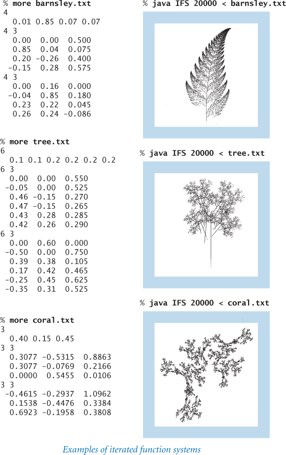
We could write code just like the code we just wrote for the Sierpinski triangle to iterate these rules, but matrix processing provides a uniform way to generalize that code to handle any set of rules. We have m different transformations, chosen from a 1-by-m vector with StdRandom.discrete(). For each transformation, we have an equation for updating x and an equation for updating y, so we use two m-by-3 matrices for the equation coefficients, one for x and one for y. IFS (PROGRAM 2.2.3) implements this data-driven version of the computation. This program enables limitless exploration: it performs the iteration for any input containing a vector that defines the probability distribution and the two matrices that define the coefficients, one for updating x and the other for updating y. For the coefficients just given, again, even though we choose a random equation at each step, the same figure emerges every time that we do this computation: an image that looks remarkably similar to a fern that you might see in the woods, not something generated by a random process on a computer.
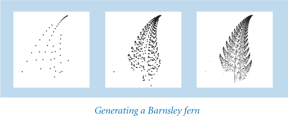
That the same short program that takes a few numbers from standard input and plots points on standard drawing can (given different data) produce both the Sierpinski triangle and the Barnsley fern (and many, many other images) is truly remarkable. Because of its simplicity and the appeal of the results, this sort of calculation is useful in making synthetic images that have a realistic appearance in computer-generated movies and games.
Perhaps more significantly, the ability to produce such realistic diagrams so easily suggests intriguing scientific questions: What does computation tell us about nature? What does nature tell us about computation?
Statistics
Next, we consider a library for a set of mathematical calculations and basic visualization tools that arise in all sorts of applications in science and engineering and are not all implemented in standard Java libraries. These calculations relate to the task of understanding the statistical properties of a set of numbers. Such a library is useful, for example, when we perform a series of scientific experiments that yield measurements of a quantity. One of the most important challenges facing modern scientists is proper analysis of such data, and computation is playing an increasingly important role in such analysis. These basic data analysis methods that we will consider are summarized in the following API:
|
||
|
|
largest value |
|
|
smallest value |
|
|
average |
|
|
sample variance |
|
|
sample standard deviation |
|
|
median |
|
|
plot points at |
|
|
plot lines connecting points at |
|
|
plot bars to points at |
Note: Overloaded implementations are included for other numeric types. |
||
API for our library of static methods for data analysis |
||
Basic statistics
Suppose that we have n measurements x0, x1, ..., xn–1. The average value of those measurements, otherwise known as the mean, is given by the formula μ = (x0 + x1 + ... + xn–1) / n and is an estimate of the value of the quantity. The minimum and maximum values are also of interest, as is the median (the value that is smaller than and larger than half the values). Also of interest is the sample variance, which is given by the formula
σ2 = ( ( x0– μ)2 + (x1 – μ)2 + ... + (xn–1 – μ)2) / (n–1)
Program 2.2.4 Data analysis library
public class StdStats
{
   public static double max(double[] a)
   {  // Compute maximum value in a[].
      double max = Double.NEGATIVE_INFINITY;
      for (int i = 0; i < a.length; i++)
         if (a[i] > max) max = a[i];
      return max;
   }

   public static double mean(double[] a)
   {  // Compute the average of the values in a[].
      double sum = 0.0;
      for (int i = 0; i < a.length; i++)
         sum = sum + a[i];
      return sum / a.length;
   }

   public static double var(double[] a)
   {  // Compute the sample variance of the values in a[].
      double avg = mean(a);
      double sum = 0.0;
      for (int i = 0; i < a.length; i++)
         sum += (a[i] - avg) * (a[i] - avg);
      return sum / (a.length - 1);
   }

   public static double stddev(double[] a)
   { return Math.sqrt(var(a)); }
   // See Program 2.2.5 for plotting methods.

   public static void main(String[] args)
   {  /* See text. */  }

}
This code implements methods to compute the maximum, mean, variance, and standard deviation of numbers in a client array. The method for computing the minimum is omitted; plotting methods are in PROGRAM 2.2.5; see EXERCISE 4.2.20 for median().
% more tiny1D.txt
5
3.0 1.0 2.0 5.0 4.0
% java StdStats < tiny1D.txt
       min   1.000
      mean   3.000
       max   5.000
   std dev   1.581
and the sample standard deviation, the square root of the sample variance. StdStats (PROGRAM 2.2.4) shows implementations of static methods for computing these basic statistics (the median is more difficult to compute than the others—we will consider the implementation of median() in SECTION 4.2). The main() test client for StdStats reads numbers from standard input into an array and calls each of the methods to print the minimum, mean, maximum, and standard deviation, as follows:
public static void main(String[] args)
{
   double[] a = StdArrayIO.readDouble1D();
   StdOut.printf("       min %7.3f
", min(a));
   StdOut.printf("      mean %7.3f
", mean(a));
   StdOut.printf("       max %7.3f
", max(a));
   StdOut.printf("   std dev %7.3f
", stddev(a));
}
As with StdRandom, a more extensive test of the calculations is called for (see EXERCISE 2.2.3). Typically, as we debug or test new methods in the library, we adjust the unit testing code accordingly, testing the methods one at a time. A mature and widely used library like StdStats also deserves a stress-testing client for extensively testing everything after any change. If you are interested in seeing what such a client might look like, you can find one for StdStats on the booksite. Most experienced programmers will advise you that any time spent doing unit testing and stress testing will more than pay for itself later.
Plotting
One important use of StdDraw is to help us visualize data rather than relying on tables of numbers. In a typical situation, we perform experiments, save the experimental data in an array, and then compare the results against a model, perhaps a mathematical function that describes the data. To expedite this process for the typical case where values of one variable are equally spaced, our StdStats library contains static methods that you can use for plotting data in an array. PROGRAM 2.2.5 is an implementation of the plotPoints(), plotLines(), and plotBars() methods for StdStats. These methods display the values in the argument array at evenly spaced intervals in the drawing window, either connected together by line segments (lines), filled circles at each value (points), or bars from the x-axis to the value (bars). They all plot the points with x-coordinate i and y-coordinate a[i] using filled circles, lines through the points, and bars, respectively. In addition, they all rescale x to fill the drawing window (so that the points are evenly spaced along the x-coordinate) and leave to the client scaling of the y-coordinates.
Program 2.2.5 Plotting data values in an array
public static void plotPoints(double[] a)
{  // Plot points at (i, a[i]).
   int n = a.length;
   StdDraw.setXscale(-1, n);
   StdDraw.setPenRadius(1/(3.0*n));
   for (int i = 0; i < n; i++)
      StdDraw.point(i, a[i]);
}

public static void plotLines(double[] a)
{  // Plot lines through points at (i, a[i]).
   int n = a.length;
   StdDraw.setXscale(-1, n);
   StdDraw.setPenRadius();
   for (int i = 1; i < n; i++)
      StdDraw.line(i-1, a[i-1], i, a[i]);
}

public static void plotBars(double[] a)
{  // Plot bars from (0, a[i]) to (i, a[i]).
   int n = a.length;
   StdDraw.setXscale(-1, n);
   for (int i = 0; i < n; i++)
      StdDraw.filledRectangle(i, a[i]/2, 0.25, a[i]/2);
}
This code implements three methods in StdStats (PROGRAM 2.2.4) for plotting data. They plot the points (i, a[i]) with filled circles, connecting line segments, and bars, respectively.
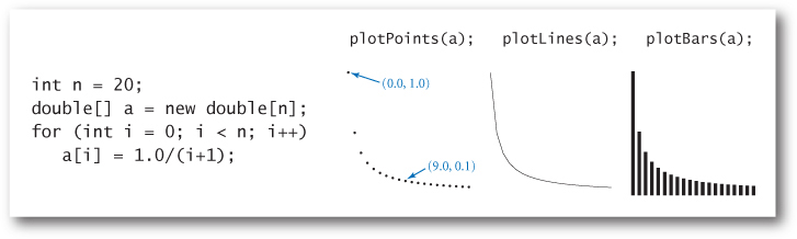
These methods are not intended to be a general-purpose plotting package, but you can certainly think of all sorts of things that you might want to add: different types of spots, labeled axes, color, and many other artifacts are commonly found in modern systems that can plot data. Some situations might call for more complicated methods than these.
Our intent with StdStats is to introduce you to data analysis while showing you how easy it is to define a library to take care of useful tasks. Indeed, this library has already proved useful—we use these plotting methods to produce the figures in this book that depict function graphs, sound waves, and experimental results. Next, we consider several examples of their use.

Plotting function graphs
You can use the StdStats.plot*() methods to draw a plot of the function graph for any function at all: choose an x-interval where you want to plot the function, compute function values evenly spaced through that interval and store them in an array, determine and set the y-scale, and then call StdStats.plotLines() or another plot*() method. For example, to plot a sine function, rescale the y-axis to cover values between –1 and +1. Scaling the x-axis is automatically handled by the StdStats methods. If you do not know the range, you can handle the situation by calling:
StdDraw.setYscale(StdStats.min(a), StdStats.max(a));
The smoothness of the curve is determined by properties of the function and by the number of points plotted. As we discussed when first considering StdDraw, you have to be careful to sample enough points to catch fluctuations in the function. We will consider another approach to plotting functions based on sampling values that are not equally spaced in SECTION 2.4.
Plotting sound waves
Both the StdAudio library and the StdStats plot methods work with arrays that contain sampled values at regular intervals. The diagrams of sound waves in SECTION 1.5 and at the beginning of this section were all produced by first scaling the y-axis with StdDraw.setYscale(-1, 1), then plotting the points with StdStats.plotPoints(). As you have seen, such plots give direct insight into processing audio. You can also produce interesting effects by plotting sound waves as you play them with StdAudio, although this task is a bit challenging because of the huge amount of data involved (see EXERCISE 1.5.23).

Plotting experimental results
You can put multiple plots on the same drawing. One typical reason to do so is to compare experimental results with a theoretical model. For example, Bernoulli (PROGRAM 2.2.6) counts the number of heads found when a fair coin is flipped n times and compares the result with the predicted Gaussian probability density function. A famous result from probability theory is that the distribution of this quantity is the binomial distribution, which is extremely well approximated by the Gaussian distribution with mean n/2 and standard deviation . The more trials we perform, the more accurate the approximation. The drawing produced by Bernoulli is a succinct summary of the results of the experiment and a convincing validation of the theory. This example is prototypical of a scientific approach to applications programming that we use often throughout this book and that you should use whenever you run an experiment. If a theoretical model that can explain your results is available, a visual plot comparing the experiment to the theory can validate both.
These few examples are intended to suggest what is possible with a well-designed library of static methods for data analysis. Several extensions and other ideas are explored in the exercises. You will find StdStats to be useful for basic plots, and you are encouraged to experiment with these implementations and to modify them or to add methods to make your own library that can draw plots of your own design. As you continue to address an ever-widening circle of programming tasks, you will naturally be drawn to the idea of developing tools like these for your own use.
Program 2.2.6 Bernoulli trials
public class Bernoulli
{
   public static int binomial(int n)
   {  // Simulate flipping a coin n times; return # heads.
      int heads = 0;
      for (int i = 0; i < n; i++)
         if (StdRandom.bernoulli(0.5)) heads++;
      return heads;
   }
   public static void main(String[] args)
   {  // Perform Bernoulli trials, plot results and model.
      int n = Integer.parseInt(args[0]);
      int trials = Integer.parseInt(args[1]);

      int[] freq = new int[n+1];
      for (int t = 0; t < trials; t++)
         freq[binomial(n)]++;

      double[] norm = new double[n+1];
      for (int i = 0; i <= n; i++)
         norm[i] = (double) freq[i] / trials;
      StdStats.plotBars(norm);

      double mean   = n / 2.0;
      double stddev = Math.sqrt(n) / 2.0;
      double[] phi = new double[n+1];
      for (int i = 0; i <= n; i++)
         phi[i] = Gaussian.pdf(i, mean, stddev);
      StdStats.plotLines(phi);
   }
}
  n    | number of flips per trial
trials | number of trials
freq[] | experimental results
norm[] | normalized results
 phi[] | Gaussian model
This StdStats, StdRandom, and Gaussian client provides visual evidence that the number of heads observed when a fair coin is flipped n times obeys a Gaussian distribution.

Modular programming
The library implementations that we have developed illustrate a programming style known as modular programming. Instead of writing a new program that is self-contained within its own file to address a new problem, we break up each task into smaller, more manageable subtasks, then implement and independently debug code that addresses each subtask. Good libraries facilitate modular programming by allowing us to define and provide solutions for important subtasks for future clients. Whenever you can clearly separate tasks within a program, you should do so. Java supports such separation by allowing us to independently debug and later use classes in separate files. Traditionally, programmers use the term module to refer to code that can be compiled and run independently; in Java, each class is a module.
IFS (PROGRAM 2.2.3) exemplifies modular programming. This relatively sophisticated computation is implemented with several relatively small modules, developed independently. It uses StdRandom and StdArrayIO, as well as the methods from Integer and StdDraw that we are accustomed to using. If we were to put all of the code required for IFS in a single file, we would have a large amount of code on our hands to maintain and debug; with modular programming, we can study iterated function systems with some confidence that the arrays are read properly and that the random number generator will produce properly distributed values, because we already implemented and tested the code for these tasks in separate modules.
API |
description |
|
Gaussian distribution functions |
|
random numbers |
|
input and output for arrays |
|
client for iterated function systems |
|
functions for data analysis |
|
client for Bernoulli trials |
Summary of classes in this section |
|
Similarly, Bernoulli (PROGRAM 2.2.6) exemplifies modular programming. It is a client of Gaussian, Integer, Math, StdRandom, and StdStats. Again, we can have some confidence that the methods in these modules produce the expected results because they are system libraries or libraries that we have tested, debugged, and used before.
To describe the relationships among modules in a modular program, we often draw a dependency graph, where we connect two class names with an arrow labeled with the name of a method if the first class contains a method call and the second class contains the definition of the method. Such diagrams play an important role because understanding the relationships among modules is necessary for proper development and maintenance.

We emphasize modular programming throughout this book because it has many important advantages that have come to be accepted as essential in modern programming, including the following:
• We can have programs of a reasonable size, even in large systems.
• Debugging is restricted to small pieces of code.
• We can reuse code without having to re-implement it.
• Maintaining (and improving) code is much simpler.
The importance of these advantages is difficult to overstate, so we will expand upon each of them.
Programs of a reasonable size
No large task is so complex that it cannot be divided into smaller subtasks. If you find yourself with a program that stretches to more than a few pages of code, you must ask yourself the following questions: Are there subtasks that could be implemented separately? Could some of these subtasks be logically grouped together in a separate library? Could other clients use this code in the future? At the other end of the range, if you find yourself with a huge number of tiny modules, you must ask yourself questions such as these: Is there some group of subtasks that logically belong in the same module? Is each module likely to be used by multiple clients? There is no hard-and-fast rule on module size: one implementation of a critically important abstraction might properly be a few lines of code, whereas another library with a large number of overloaded methods might properly stretch to hundreds of lines of code.
Debugging
Tracing a program rapidly becomes more difficult as the number of statements and interacting variables increases. Tracing a program with hundreds of variables requires keeping track of hundreds of values, as any statement might affect or be affected by any variable. To do so for hundreds or thousands of statements or more is untenable. With modular programming and our guiding principle of keeping the scope of variables local to the extent possible, we severely restrict the number of possibilities that we have to consider when debugging. Equally important is the idea of a contract between client and implementation. Once we are satisfied that an implementation is meeting its end of the bargain, we can debug all its clients under that assumption.
Code reuse
Once we have implemented libraries such as StdStats and StdRandom, we do not have to worry about writing code to compute averages or standard deviations or to generate random numbers again—we can simply reuse the code that we have written. Moreover, we do not need to make copies of the code: any module can just refer to any public method in any other module.
Maintenance
Like a good piece of writing, a good program can always be improved, and modular programming facilitates the process of continually improving your Java programs because improving a module improves all of its clients. For example, it is normally the case that there are several different approaches to solving a particular problem. With modular programming, you can implement more than one and try them independently. More importantly, suppose that while developing a new client, you find a bug in some module. With modular programming, fixing that bug essentially fixes bugs in all of the module’s clients.
If you encounter an old program (or a new program written by an old programmer!), you are likely to find one huge module—a long sequence of statements, stretching to several pages or more, where any statement can refer to any variable in the program. Old programs of this kind are found in critical parts of our computational infrastructure (for example, some nuclear power plants and some banks) precisely because the programmers charged with maintaining them cannot even understand them well enough to rewrite them in a modern language! With support for modular programming, modern languages like Java help us avoid such situations by separately developing libraries of methods in independent classes.
The ability to share static methods among different files fundamentally extends our programming model in two different ways. First, it allows us to reuse code without having to maintain multiple copies of it. Second, by allowing us to organize a program into files of manageable size that can be independently debugged and compiled, it strongly supports our basic message: whenever you can clearly separate tasks within a program, you should do so.
In this section, we have supplemented the Std* libraries of SECTION 1.5 with several other libraries that you can use: Gaussian, StdArrayIO, StdRandom, and StdStats. Furthermore, we have illustrated their use with several client programs. These tools are centered on basic mathematical concepts that arise in any scientific project or engineering task. Our intent is not just to provide tools, but also to illustrate that it is easy to create your own tools. The first question that most modern programmers ask when addressing a complex task is “Which tools do I need?” When the needed tools are not conveniently available, the second question is “How difficult would it be to implement them?” To be a good programmer, you need to have the confidence to build a software tool when you need it and the wisdom to know when it might be better to seek a solution in a library.
After libraries and modular programming, you have one more step to learn a complete modern programming model: object-oriented programming, the topic of CHAPTER 3. With object-oriented programming, you can build libraries of functions that use side effects (in a tightly controlled manner) to vastly extend the Java programming model. Before moving to object-oriented programming, we consider in this chapter the profound ramifications of the idea that any method can call itself (in SECTION 2.3) and a more extensive case study (in SECTION 2.4) of modular programming than the small clients in this section.
Q&A
Q. I tried to use StdRandom, but got the error message Exception in thread "main" java.lang.NoClassDefFoundError: StdRandom. What’s wrong?
A. You need to make StdRandom accessible to Java. See the first Q&A at the end of SECTION 1.5.
Q. Is there a keyword that identifies a class as a library?
A. No, any set of public methods will do. There is a bit of a conceptual leap in this viewpoint because it is one thing to sit down to create a .java file that you will compile and run, quite another thing to create a .java file that you will rely on much later in the future, and still another thing to create a .java file for someone else to use in the future. You need to develop some libraries for your own use before engaging in this sort of activity, which is the province of experienced systems programmers.
Q. How do I develop a new version of a library that I have been using for a while?
A. With care. Any change to the API might break any client program, so it is best to work in a separate directory. When you use this approach, you are working with a copy of the code. If you are changing a library that has a lot of clients, you can appreciate the problems faced by companies putting out new versions of their software. If you just want to add a few methods to a library, go ahead: that is usually not too dangerous, though you should realize that you might find yourself in a situation where you have to support that library for years!
Q. How do I know that an implementation behaves properly? Why not automatically check that it satisfies the API?
A. We use informal specifications because writing a detailed specification is not much different from writing a program. Moreover, a fundamental tenet of theoretical computer science says that doing so does not even solve the basic problem, because generally there is no way to check that two different programs perform the same computation.
Exercises
2.2.1 Add to Gaussian (PROGRAM 2.1.2) an implementation of the three-argument static method pdf(x, mu, sigma) specified in the API that computes the Gaussian probability density function with a given mean μ and standard deviation σ, based on the formula ϕ(x, μ, σ) = ϕ((x– μ) / σ)/σ. Also add an implementation of the associated cumulative distribution function cdf(z, mu, sigma), based on the formula Φ(z, μ, σ) = Φ((z – μ) / σ).
2.2.2 Write a library of static methods that implements the hyperbolic functions based on the definitions sinh(x) = (ex – e–x) / 2 and cosh(x) = (ex + e–x) / 2, with tanh(x), coth(x), sech(x), and csch(x) defined in a manner analogous to standard trigonometric functions.
2.2.3 Write a test client for both StdStats and StdRandom that checks that the methods in both libraries operate as expected. Take a command-line argument n, generate n random numbers using each of the methods in StdRandom, and print their statistics. Extra credit: Defend the results that you get by comparing them to those that are to be expected from analysis.
2.2.4 Add to StdRandom a method shuffle() that takes an array of double values as argument and rearranges them in random order. Implement a test client that checks that each permutation of the array is produced about the same number of times. Add overloaded methods that take arrays of integers and strings.
2.2.5 Develop a client that does stress testing for StdRandom. Pay particular attention to discrete(). For example, do the probabilities sum to 1?
2.2.6 Write a static method that takes double values ymin and ymax (with ymin strictly less than ymax), and a double array a[] as arguments and uses the StdStats library to linearly scale the values in a[] so that they are all between ymin and ymax.
2.2.7 Write a Gaussian and StdStats client that explores the effects of changing the mean and standard deviation for the Gaussian probability density function. Create one plot with the Gaussian distributions having a fixed mean and various standard deviations and another with Gaussian distributions having a fixed standard deviation and various means.
2.2.8 Add a method exp() to StdRandom that takes an argument λ and returns a random number drawn from the exponential distribution with rate λ. Hint: If x is a random number uniformly distributed between 0 and 1, then –ln x / λ is a random number from the exponential distribution with rate λ.
2.2.9 Add to StdRandom a static method maxwellBoltzmann() that returns a random value drawn from a Maxwell–Boltzmann distribution with parameter σ. To produce such a value, return the square root of the sum of the squares of three random numbers drawn from the Gaussian distribution with mean 0 and standard deviation σ. The speeds of molecules in an ideal gas obey a Maxwell–Boltzmann distribution.
2.2.10 Modify Bernoulli (PROGRAM 2.2.6) to animate the bar graph, replotting it after each experiment, so that you can watch it converge to the Gaussian distribution. Then add a command-line argument and an overloaded binomial() implementation to allow you to specify the probability p that a biased coin comes up heads, and run experiments to get a feeling for the distribution corresponding to a biased coin. Be sure to try values of p that are close to 0 and close to 1.
2.2.11 Develop a full implementation of StdArrayIO (implement all 12 methods indicated in the API).
2.2.12 Write a library Matrix that implements the following API:
|
||
|
|
vector dot product |
|
|
matrix–matrix product |
|
|
transpose |
|
|
matrix–vector product |
|
|
vector–matrix product |
(See SECTION 1.4.) As a test client, use the following code, which performs the same calculation as Markov (PROGRAM 1.6.3):
public static void main(String[] args)
{
   int trials = Integer.parseInt(args[0]);
   double[][] p = StdArrayIO.readDouble2D();
   double[] ranks = new double[p.length];
   rank[0] = 1.0;
   for (int t = 0; t < trials; t++)
       ranks = Matrix.multiply(ranks, p);
   StdArrayIO.print(ranks);
}
Mathematicians and scientists use mature libraries or special-purpose matrix-processing languages for such tasks. See the booksite for details on using such libraries.
2.2.13 Write a Matrix client that implements the version of Markov described in SECTION 1.6 but is based on squaring the matrix, instead of iterating the vector–matrix multiplication.
2.2.14 Rewrite RandomSurfer (PROGRAM 1.6.2) using the StdArrayIO and StdRandom libraries.
Partial solution.
...
double[][] p = StdArrayIO.readDouble2D();
int page = 0; // Start at page 0.
int[] freq = new int[n];
for (int t = 0; t < trials; t++)
{
   page = StdRandom.discrete(p[page]);
   freq[page]++;
}
...
Creative Exercises
2.2.15 Sicherman dice. Suppose that you have two six-sided dice, one with faces labeled 1, 3, 4, 5, 6, and 8 and the other with faces labeled 1, 2, 2, 3, 3, and 4. Compare the probabilities of occurrence of each of the values of the sum of the dice with those for a standard pair of dice. Use StdRandom and StdStats.
2.2.16 Craps. The following are the rules for a pass bet in the game of craps. Roll two six-sided dice, and let x be their sum.
• If x is 7 or 11, you win.
• If x is 2, 3, or 12, you lose.
Otherwise, repeatedly roll the two dice until their sum is either x or 7.
• If their sum is x, you win.
• If their sum is 7, you lose.
Write a modular program to estimate the probability of winning a pass bet. Modify your program to handle loaded dice, where the probability of a die landing on 1 is taken from the command line, the probability of landing on 6 is 1/6 minus that probability, and 2–5 are assumed equally likely. Hint: Use StdRandom.discrete().
2.2.17 Gaussian random values. Implement the no-argument gaussian() function in StdRandom (PROGRAM 2.2.1) using the Box–Muller formula (see EXERCISE 1.2.27). Next, consider an alternative approach, known as Marsaglia’s method, which is based on generating a random point in the unit circle and using a form of the Box–Muller formula (see the discussion of do-while at the end of SECTION 1.3).
public static double gaussian()
{
   double r, x, y;
   do
   {
      x = uniform(-1.0, 1.0);
      y = uniform(-1.0, 1.0);
      r = x*x + y*y;
   } while (r >= 1 || r == 0);
   return x * Math.sqrt(-2 * Math.log(r) / r);
}
For each approach, generate 10 million random values from the Gaussian distribution, and measure which is faster.
2.2.18 Dynamic histogram. Suppose that the standard input stream is a sequence of double values. Write a program that takes an integer n and two double values lo and hi from the command line and uses StdStats to plot a histogram of the count of the numbers in the standard input stream that fall in each of the n intervals defined by dividing (lo, hi) into n equal-sized intervals. Use your program to add code to your solution to EXERCISE 2.2.3 to plot a histogram of the distribution of the numbers produced by each method, taking n from the command line.
2.2.19 Stress test. Develop a client that does stress testing for StdStats. Work with a classmate, with one person writing code and the other testing it.
2.2.20 Gambler’s ruin. Develop a StdRandom client to study the gambler’s ruin problem (see PROGRAM 1.3.8 and EXERCISE 1.3.24–25). Note: Defining a static method for the experiment is more difficult than for Bernoulli because you cannot return two values.
2.2.21 IFS. Experiment with various inputs to IFS to create patterns of your own design like the Sierpinski triangle, the Barnsley fern, or the other examples in the table in the text. You might begin by experimenting with minor modifications to the given inputs.
2.2.22 IFS matrix implementation. Write a version of IFS that uses the static method multiply() from Matrix (see EXERCISE 2.2.12) instead of the equations that compute the new values of x0 and y0.
2.2.23 Library for properties of integers. Develop a library based on the functions that we have considered in this book for computing properties of integers. Include functions for determining whether a given integer is prime; determining whether two integers are relatively prime; computing all the factors of a given integer; computing the greatest common divisor and least common multiple of two integers; Euler’s totient function (EXERCISE 2.1.26); and any other functions that you think might be useful. Include overloaded implementations for long values. Create an API, a client that performs stress testing, and clients that solve several of the exercises earlier in this book.
2.2.24 Music library. Develop a library based on the functions in PlayThatTune (PROGRAM 2.1.4) that you can use to write client programs to create and manipulate songs.
2.2.25 Voting machines. Develop a StdRandom client (with appropriate static methods of its own) to study the following problem: Suppose that in a population of 100 million voters, 51% vote for candidate A and 49% vote for candidate B. However, the voting machines are prone to make mistakes, and 5% of the time they produce the wrong answer. Assuming the errors are made independently and at random, is a 5% error rate enough to invalidate the results of a close election? What error rate can be tolerated?
2.2.26 Poker analysis. Write a StdRandom and StdStats client (with appropriate static methods of its own) to estimate the probabilities of getting one pair, two pair, three of a kind, a full house, and a flush in a five-card poker hand via simulation. Divide your program into appropriate static methods and defend your design decisions. Extra credit: Add straight and straight flush to the list of possibilities.
2.2.27 Animated plots. Write a program that takes a command-line argument m and produces a bar graph of the m most recent double values on standard input. Use the same animation technique that we used for BouncingBall (PROGRAM 1.5.6): erase, redraw, show, and wait briefly. Each time your program reads a new number, it should redraw the whole bar graph. Since most of the picture does not change as it is redrawn slightly to the left, your program will produce the effect of a fixed-size window dynamically sliding over the input values. Use your program to plot a huge time-variant data file, such as stock prices.
2.2.28 Array plot library. Develop your own plot methods that improve upon those in StdStats. Be creative! Try to make a plotting library that you think will be useful for some application in the future.