Chapter Five. Modeling and Design
Objectives
After studying the material in this chapter, you should be able to:
1. Describe modeling methods available to represent your design.
2. List model qualities that can help you select among them.
3. Describe how models can be used in refining designs.
4. Describe which modeling method contains the most information about a design.
5. Describe how a constraint-based modeler differs from a traditional solid modeler.
6. Define design intent and how it is reflected in a constraint-based model.
7. Define the basic functions of a constraint-based modeler.
8. Identify the role of a base feature.
9. Identify constraint relationships and driving dimensions.
Refer to the following standards:
• ANSI/ASME Y14.100 Engineering Drawing Practices
• ASME Y14.41 Digital Product Definition Data Practices
The ENV hydrogen fuel cell motorbike was designed from the fuel cell outward. During its development many refinements were made both technologically and visually. Models in this phase must represent the design accurately enough to be used for testing as well as to convey the details of the design for implementation. (Courtesy of Seymourpowell.)
Refinement and Modeling
From the solutions generated during ideation, only a few are selected for further consideration. The design review process determines whether money will be committed for further development of a design.
The process of refining and analyzing the design is iterative. As the refined design is tested, the test results suggest modifications to the design, and once the design is changed, it needs further analysis.
Creating a CAD model is an important step in the refinement process. A huge amount of design information can be stored in CAD models that are easily modified. The CAD model can be used to test and evaluate the design. By making changes easy—and in some cases, automating the update process—CAD modeling can eliminate some barriers to a thorough review and refinement of the design.
CAD models also encourage refinement by making it easier and less costly to get feedback about a design while it is in development. Accurate part descriptions allow you to test how well parts will fit together. Customer acceptance and styling issues can be assessed early in the design process using realistically shaded models. Analysis programs can import 3D CAD files or run as part of the CAD software, saving much time. Some analysis packages suggest optimizations to incorporate directly in the CAD model. Animation and kinematic analysis uses CAD data to determine whether the design will function properly before any parts are actually built.
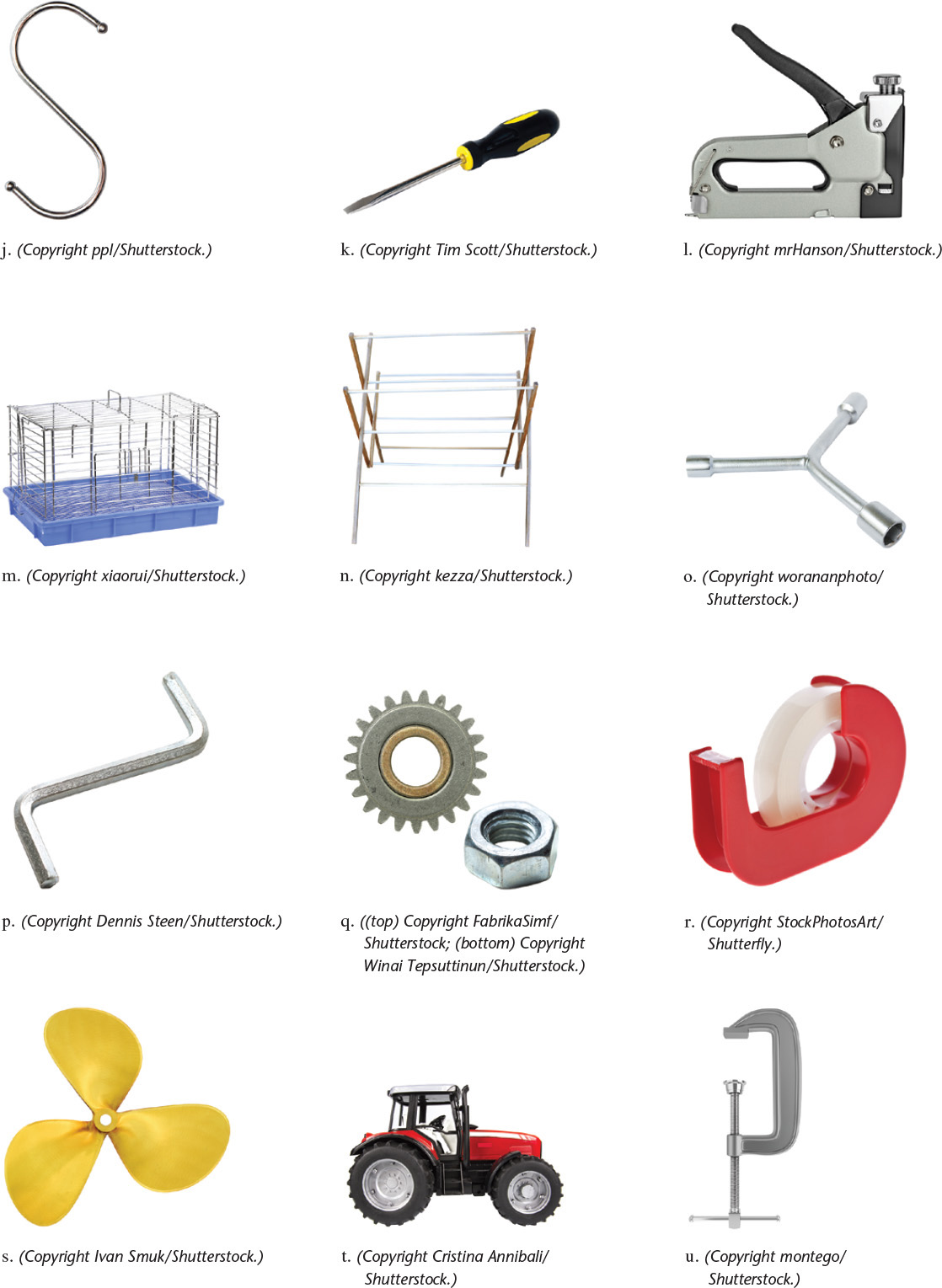
Many different methods are used to create CAD models, each with its strengths and weaknesses for capturing design information. Each item shown in Figure 5.1 may be modeled differently, possibly requiring different software and techniques.
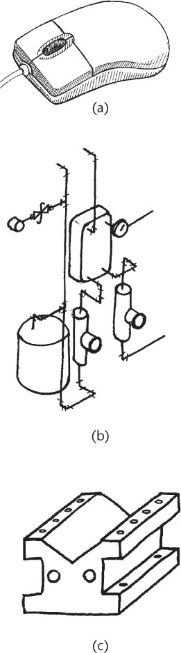
5.1 The same modeling software may be used to model (a) the ergonomic mouse, (b) the piping system, and (c) the V-block, but different modeling methods may be best suited to each.
In this chapter, you will learn how different modeling methods represent and store design information, and the advantages and disadvantages of each. This information will aid you in choosing the most effective method for a particular design problem.
Descriptive Models
Descriptive models represent a system or device in either words or pictures. Descriptive models sometimes use representations that are simplified or analogous to something that is more easily understood. The key function of a descriptive model is to describe, that is, to provide enough detail to convey an image of the final product.
A set of written specifications for a design is a descriptive model. If all the specifications are followed, the system will perform correctly. Sketching is also a type of descriptive model for your design ideas on paper. 2D and 3D CAD drawings are also descriptive models. A physical model or prototype is another type of descriptive model, although sometimes physical models are made to a smaller scale (called a scale model).
The figures at right show a scale model of a design for the Next Generation Space Telescope (NGST) developed by NASA. A model helps you visualize the design. It has the added benefit of being easy for non-engineers to understand while decisions are being made about the next step in the project.
Spotlight: A 1:10 Scale Model
This scale model represents a design by Ball Aerospace for the Next Generation Space Telescope (NGST). The mock-up was the largest and most complex scale model created by Ball Aerospace. At 1:10 scale, it represents a telescope that stands over 9 feet tall with a primary mirror 8 meters in diameter when fully deployed (Figure b). Because the primary mirror is so large, it must be able to fold in on itself to fit inside a launch vehicle, as shown in Figure a. This scale model demonstrated the deployment using seventeen computer-controlled motors. Because of the improbability of servicing this telescope in space, this design is also partially functional even if the mirrors fail to fully deploy.
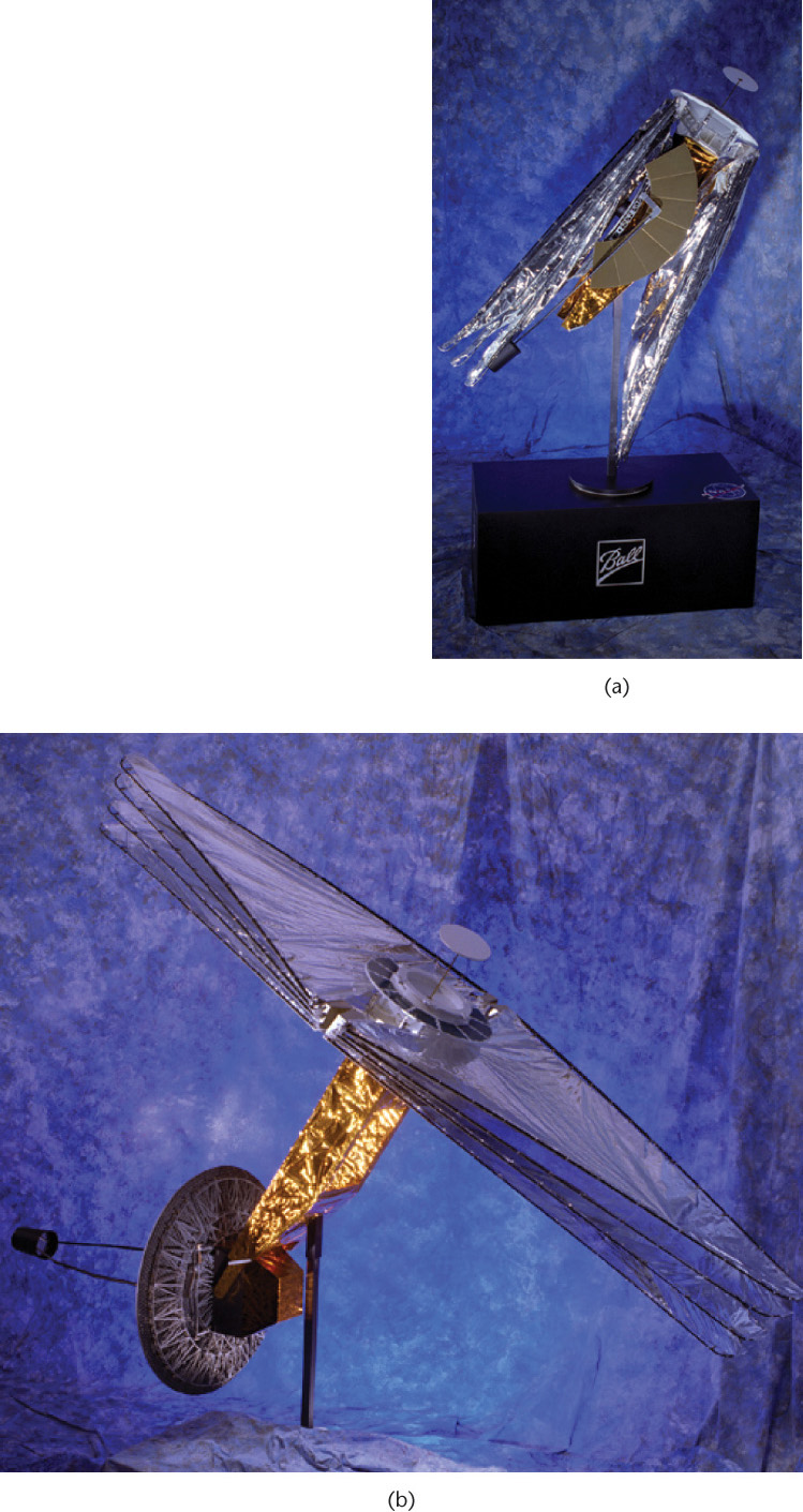
(Photos courtesy of Ball Aerospace & Technologies Corporation.)
Analytical Models
An analytical model captures the behavior of the system or device in a mathematical expression or schematic that can be used to predict future behavior. The electrical circuit model shown in Figure 5.2 is an example of an analytical model. The circuit and its properties are represented in the model by equations and relations that simulate the way the component would behave in a real circuit. The designer can change values to make predictions about what will happen in a real circuit that is wired the same way as the model. This makes it easier, less expensive, and faster to test the design.
5.2 A simple circuit design model allows simulation of its function. (Courtesy of Cadence® Design Systems, Inc.)
Part of creating an effective analytical model is determining which aspects of the system’s behavior to model. In the circuit model, some information, such as interference between some components, is left out because it is too complex to represent effectively. A finite element analysis (FEA) model, such as that used to generate the stress plot shown in Figure 5.3a, simplifies the CAD model in a similar way. The FEA model breaks the model into smaller elements; reducing a complicated system to a series of smaller systems allows the stresses more easily to be solved. Understanding and using analytical models effectively requires knowing how the model differs from the actual system so the results can be interpreted correctly.
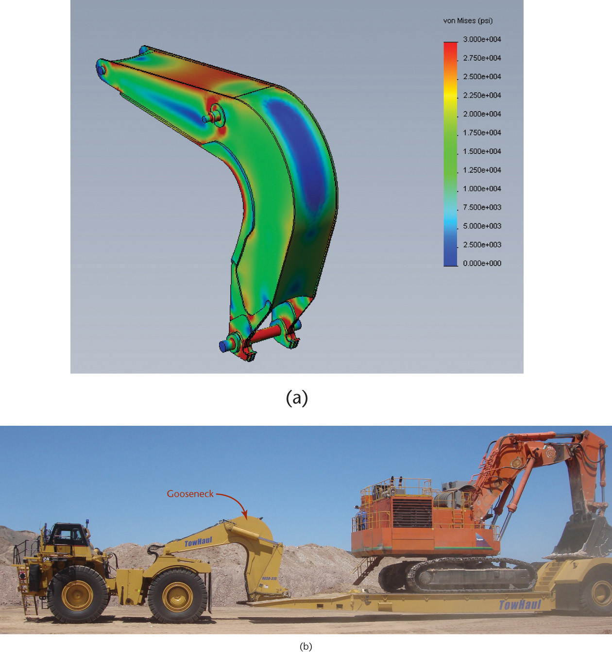
5.3 Finite element analysis (a) is used to calculate the stresses on the gooseneck shown in (b) in designing this heavy-duty equipment. (Courtesy of TowHaul Corporation.)
In the design process, use different types of models where they are appropriate. During the ideation phase of the design, sketching is often the best technique to use. As you begin to refine the design, you will use both descriptive and analytical models to represent the design more accurately and to provide insight into its behavior.
A 3D CAD model combines qualities of descriptive and analytical models. Because a 3D CAD model accurately depicts the geometry of a device, it can fully describe its shape, size, and appearance as a physical or scale model would. Additional information about the final product, such as the materials from which it will be made, can also be added to the model description stored in the computer database. Figure 5.4 shows a CAD model of NASA’s Space Infrared Telescope Facility (SIRTF).
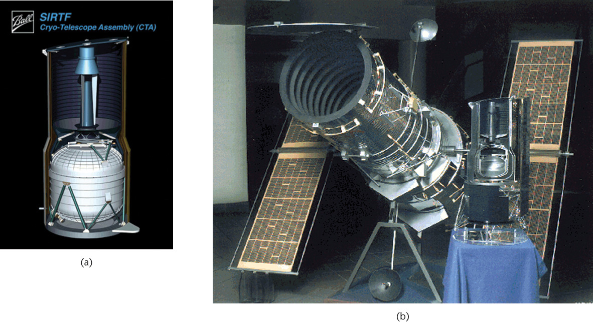
5.4 Descriptive and Analytical. This rendered view of the preliminary CAD model of the SIRTF assembly, shown in (a), looks very similar to the photograph of its 1:10 scale model, shown in (b) next to a 1:10 model of the Hubble Space Telescope. (Courtesy of Ball Aerospace and Technologies Corporation.)
A 3D CAD model can also be used for analytical modeling. The 3D model of the device can be used to study its characteristics (see Figure 5.5). Sophisticated software allows you to analyze, animate, and predict the behavior of the design under various physical conditions. The 3D CAD model is a detailed representation of the final object, suited for testing and study.

5.5 Motion Analysis. These welding robots are programmed with code developed with 3D model data. The motion of the robots is simulated with a 3D model of the part to be welded and 3D models of the robots. Motion paths are then exported and used to program the actual robots. (Courtesy of FANUC America Corporation.)
5.1 2D Models
Paper Drawings
2D sketches and multiview drawings are representations of the design. All the information defining the object may be shown in a paper drawing (see Figure 5.6), although it may require many orthographic views.

5.6 This fully dimensioned paper drawing contains all the information needed to manufacture this part, which will be flame cut from a 96 × 156-inch sheet of steel. (Courtesy of Smith Equipment, USA.)
Multiview drawing techniques were designed to improve the robustness, measurability, and accuracy of paper drawings. These same techniques require some skill to be understood, however, and make multiview drawings harder to understand than a 3D model.
Equipment costs for paper drawings are minimal, but they take as long or longer to create than CAD drawings. Changes involve considerable erasing and redrawing, making them difficult to modify as the design changes. Because paper drawings are difficult to change, the labor costs associated with them usually outweigh the equipment savings.
Paper drawing accuracy is about plus or minus one fortieth the drawing scale. For example, a paper drawing of a map drawn at a scale of 1 inch = 400 feet has good accuracy if you can measure from it to plus or minus 10 feet. This makes paper drawings not particularly measurable or accurate—which is why proper dimensioning technique was developed. Proper dimensioning overcomes this limitation and provides measurements to the desired accuracy on the drawing. It is not good practice to make measurements from paper drawings.
Paper drawings can be very effective for quickly communicating the design of small parts for manufacturing. A properly dimensioned sketch can quickly convey all the information needed to make a part that is needed only one time (see Figure 5.7). Also, manufacturing facilities occasionally are not able to read electronic files and require paper drawings.

2D CAD Models
2D CAD models share the visual characteristics of paper drawings but are more accurate and easier to change. CAD systems have a large variety of editing tools that allow quick editing and reuse of drawing geometry. Standard symbols are easy to add and change.
2D CAD drawings can quickly be printed to different scales. Different types of information can be separated onto different layers that can either be displayed or turned off, making the model more flexible than a paper drawing.
Using CAD, you can accurately define the locations of lines, arcs, and other geometry. In AutoCAD, for example, you can store these locations to at least fourteen decimal places. You can query the database, and the information will be returned as accurately as you originally created it. Of course, the adage Garbage In, Garbage Out (GIGO) applies. If your endpoints do not connect, or you locate distances by eye instead of entering them precisely, you will not have accurate results.
CAD models represent the object full size, unlike paper drawings, so you can make measurements and calculations from 2D CAD models. Also, you can “snap” to locations on objects to determine sizes and distances that may not be dimensioned on a paper drawing. If there must be a clearance of 10 feet from the center of a tank to the location of another piece of equipment, you can measure from the CAD file to determine whether proper clearance is provided in the design.
Text and other information can be saved in a database and linked to the drawing information for later retrieval. The 2D database is limited, however, in its ability to represent information that depends on a 3D definition (such as the volume inside the object), so it is not generally useful for determining mass and other physical properties of the object.
The strengths and weaknesses of paper drawing are shared by 2D CAD models. To create them and read them you must be able to interpret the 2D views to “see” the 3D object. To measure from a 2D CAD model, you must show distances and angles true length in a view. Orthographic projection and descriptive geometry are needed to create these views. Descriptive geometry is the study of producing views of an object that show true lengths, shape, angles, and other information about an engineering design. Mastering these subjects enables you to use auxiliary views created with a 2D CAD system along with the traditional methods of descriptive geometry to solve many engineering problems.
Flexibility and accuracy make 2D CAD systems a cost-effective tool in a wide variety of businesses. For many civil engineering projects, the difficulty of capturing all the 3D information needed to model irregular surfaces, such as terrain, may not be worth the benefits of working in 3D. For projects such as highway design, civil mapping, electrical distribution, and building systems, 2D CAD models may provide enough information and be created more quickly from the information at hand (see Figure 5.8). Areas and perimeters can be calculated accurately, and drawings can be revised quickly. 2D CAD models are more accurate than paper drawings.
5.8 Large-scale projects such as this highway plan are often modeled in 2D CAD. Most 2D CAD systems associate dimension values with the entities they describe, so dimensions can be updated if the drawing changes. (Courtesy of Montana Department of Transportation, MSU Design Section, Bozeman, MT.)
If lines and shapes in a 2D CAD drawing are not drawn using methods that connect exact geometry, they may not actually connect. This can cause a number of different problems. For example, when crosshatching inside a boundary, even a small gap can cause the hatching to “leak” out.
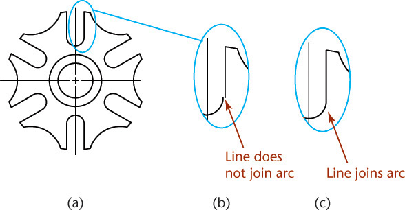
The drawing of the geneva cam below appears fine here and on screen. But when the corner is enlarged, it is clear that the line that should be tangent to the arc does not connect. Because of the algorithm used to generate circles and arcs, line segments used to represent them may not appear to connect when zoomed. But when the CAD drawing is regenerated from the data in the file, the line will—if tangent—clearly touch the arc, as shown in (c).
2D Constraint-Based Modeling
Constraint-based modeling originally started as a method for creating 3D models. Constraint-based 2D models provide a mechanism for defining a 2D shape based on its geometry. Relationships like concentricity and tangency can be added between entities in the drawing. For example, once a concentric constraint is added between two circles, they will remain concentric, and you will be alerted if you attempt to make a change that will violate this geometric constraint. Dimensions in the drawing constrain the sizes of features.
Relationships defined between parts of the 2D model are maintained by the software when you make changes to the drawing. Geometric constraints can be a valuable tool, but to benefit from them, you must apply them with a good understanding of basic drawing geometry and the behavior desired when changes are made to the shape.
2D Constraints: 2D Constraints in AutoCAD 2016
2D drawing geometry defined using constraints must behave so as to satisfy the conditions placed on the drawing elements. Small constraint symbols indicate on-screen which conditions have been defined for the shape. The following constraints are available for defining AutoCAD geometry:
• Horizontal: Lines or pairs of points on objects must remain parallel to the X-axis.
• Vertical: Lines or pairs of points on objects must remain parallel to the Y-axis.
• Perpendicular: Two selected lines must maintain a 90° angle to one another.
• Parallel: Two selected lines must remain parallel.
• Tangent: Two curves must maintain tangency to each other or to their extensions.
• Smooth: A spline must be contiguous and maintain G2 curvature continuity with another entity.
• Coincident: Two points must stay connected.
• Concentric: Two arcs, circles, or ellipses must maintain the same center point.
• Collinear: Two or more line segments must remain along the same line.
• Symmetric: Two selected objects must remain symmetrical about a specified line.
• Equal: Selected entities must maintain the same size.
• Fix: Points, line endpoints, or curve points must stay in fixed position on the coordinate system.
The following size constraints are also available:
• Linear: The distance between two points along the X- or Y-axis must be maintained.
• Aligned: A distance between two points must be maintained.
• Radius: The radius for a curve must be maintained.
• Diameter: The diameter of a circle must be maintained.
• Angular: The angle between two lines must be maintained.

(Autodesk screen shots reprinted courtesy of Autodesk, Inc.)
5.2 3D Models
2D models must be interpreted to visualize a 3D object. To convey the design to individuals unfamiliar with orthographic projection—or to evaluate properties of the design that are undefined in 2D representations—3D models are used.
Physical Models
Physical models provide an easy visual reference. Physical models are called prototypes when they are made full size or used to validate a nearly final design for production. People can interact with them and get a feel for how the design will look and how it will function. Many problems with designs are discovered and corrected when a physical prototype is made.
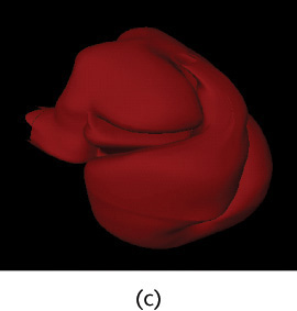
The robustness and cost effectiveness of physical models are often linked. A simple model made of clay or cardboard may be enough for some purposes (see Figure 5.9), but determining the fit of many parts in a large-scale assembly, or producing a model realistic enough for market testing, may be cost prohibitive until very late in the design process. A full-size prototype of the BMW 850I cost more than $1 million to produce. The amount of information and detail built into the model adds to its cost.
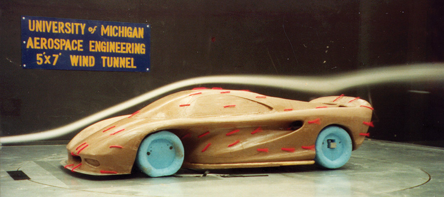
5.9 This physical clay model of the Romulus Predator was used to evaluate the aerodynamics of its lines in a wind tunnel at the University of Michigan. (Courtesy of Mark Gerisch.)
The accuracy of a physical prototype also drives up its cost. Many objects are designed to be mass produced so that the cost of individual parts is reduced. When each part in the model must be produced one at a time, the cost of the prototype can be many times greater than the manufacturing cost of the final product. The more the model must match the final product in terms of materials used and final appearance, the greater the cost. Rapid prototyping systems offer quick and relatively inexpensive means of generating a physical model of smaller parts without the cost of machining or forming parts one at a time (see Figure 5.10).

5.10 Prototype parts created using a fused deposition modeling system are useful for design verification. (Courtesy of Stratsys, Inc.)
Physical models are a very good visual representation of the design, but if they are not made from the materials that will be selected for the design, their weight and other characteristics will not match the final product. Sometimes, owing to the size of the project, the physical model must be made to a smaller scale than the final design. The accuracy of the final part also may not be possible with the materials and processes used for the prototype.
Probably the least attractive feature of a physical prototype is its lack of flexibility. Once a physical prototype has been created, changing it is expensive, difficult, and time-consuming. Consequently, full-size physical models are not usually used until fairly late in the design process—when major design changes are less likely. This can limit the usefulness of the model even though it provides important feedback about items that are not working well. When the information comes late in the design process, it can be too expensive to return to a much earlier stage of the design to pursue a different approach. Only critical problems may be fixed. Solutions to problems found late in the process are generally constrained to cause the least amount of redesign while fixing the problem. When a prototype is created late in the process, there may not be time or resources to create a new prototype for the new solution. New problems introduced by the change may not be seen until actual parts are produced.
Despite the trade-offs, even very costly physical models have been a cost-effective way for companies to avoid much more costly errors in manufacturing.
3D CAD Models
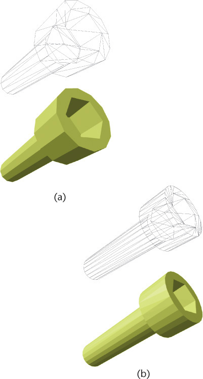
A 3D CAD model offers all the benefits of a 2D model and a physical model. As a visual representation, 3D CAD models can generate standard 2D multiview drawings as well as realistically shaded and rendered views. Because a 3D CAD model accurately depicts the geometry of the device, it may eliminate the need for a prototype—or make it easy to create one from the data stored in the model. Options for viewing the model make it understandable to a wide range of individuals who might be involved with the design’s refinement (see Figure 5.11).
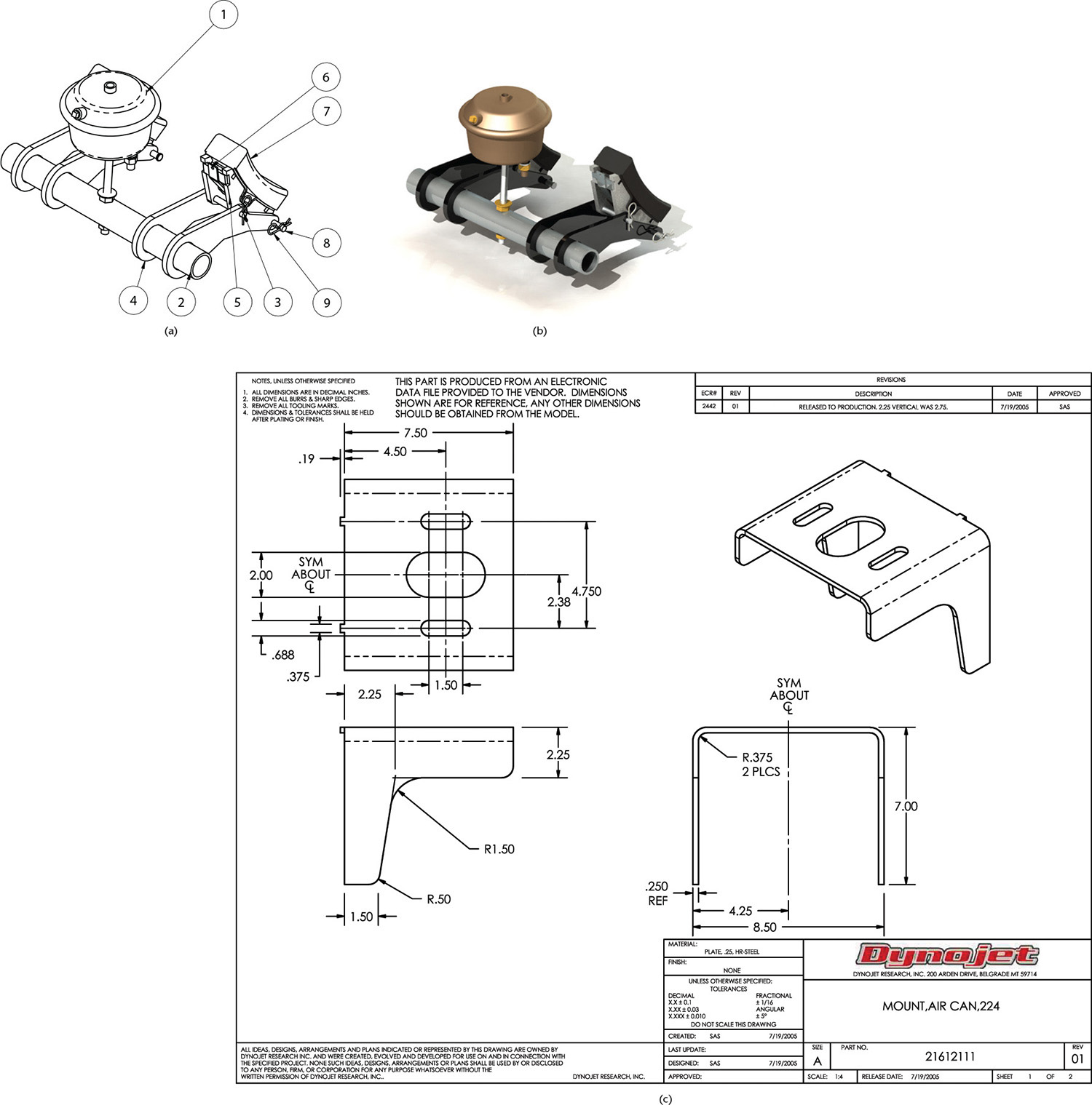
5.11 The 3D model, shown as outline in (a), can also be rendered to produce the realistic view shown in (b) and to generate accurate 2D views for multiview drawings (c). (Courtesy of Dynojet Research, Inc.)
Virtual Reality
Virtual reality (VR) refers to interacting with a 3D CAD model as if it were real—the model simulates the way the user would interact with a real device or system. Using a virtual reality display, users are immersed in the model so that they can move around (and sometimes through) it and see it from different points of view. The headset display shown in Figure 5.12 uses two displays set about 3 inches apart (the typical distance between a person’s eyes). Each display shows a view of the object as it would be seen from the eye looking at it, which creates a stereoscopic view similar to the one sent to the brain by our two eyes. Some headsets let you control the viewpoint by moving your eyes or head, so that as you look around, a new view is created to correspond with the new direction.

5.12 Virtual Reality Headset. Cybermind’s Visette45 has both closed and see-through versions offering an effective screen size of 80 inches at 2 meters. (Courtesy of Cinoptics.)
Some 3D interfaces, such as a 3D mouse or controller, let the user interact with the items in the 3D model in a way that enhances the illusion of reality. Some gloves (similar to those shown in Figure 5.13) even use model data to provide physical feedback to the user when an object is encountered. If a virtual object is squeezed, feedback to the glove provides the feeling of the resistance a solid object would give when squeezed. Systems may even interpret how much force would crush the object and provide this sensation to the user.
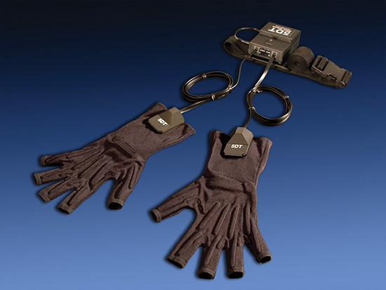
5.13 Virtual Reality Gloves. These 5DT Ultra series of data gloves are controlled via a belt-worn wireless kit designed to transmit data for two gloves simultaneously. (Courtesy of 5DT/Fifth Dimension Technologies.)
The term virtual prototype describes 3D CAD systems that represent the object realistically enough for users, designers, and manufacturers to get the same type of information they get from creating a physical prototype.
As more sophisticated software becomes available to analyze, animate, and predict the behavior of the design under various physical conditions, the 3D CAD model becomes a better representation of the final object—and better suited for testing and study.
3D CAD models offer a high degree of accuracy and measurability and a high degree of flexibility. Each new generation of CAD software automates more common tasks, allowing the designer to focus more on the design and less on the mechanics of changing the model. This flexibility allows the CAD model to become a preliminary work that is refined and tested until it is ready to be used as a plan for the final product.
The ability of 3D CAD models to be used throughout the process, serve in lieu of a physical model, and be reused and modified indefinitely makes them very cost effective, especially in designing mechanical assemblies. However, not all 3D CAD models are the same. Familiarity with different types of 3D modeling systems lets you select the method and software most suitable for your design project.
5.3 Types of 3D Models
Each of the major 3D modeling methods—wireframe modeling, surface modeling, solid modeling, and parametric constraint-based modeling—has its advantages and disadvantages. Many CAD systems incorporate all these modeling methods into one single software package. Other software may provide only one or two of these methods.
Wireframe Models
Wireframe modeling represents the edges and contours of an object using lines, circles, and arcs oriented in 3D space. 3D wireframe drawings can be easy to create, are handled by many low-cost software packages, and provide a good tool for modeling simple 3D shapes. The method gets its name from the appearance of the model, which resembles a sculpture made of wires, as shown in Figure 5.14.
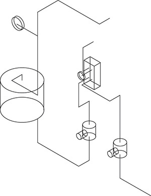
5.14 A Wireframe Model. Edges and contours of an object are represented by lines, circles, and arcs oriented in 3D space. 3D wireframe is a suitable method for modeling this snow-melting system.
You create a wireframe model in much the same way that you create a 2D CAD drawing. Each edge where surfaces on the object intersect is drawn in 3D space using simple geometric tools, such as a 3D line or arc. The X-, Y-, and Z-coordinates for the endpoints are stored in the database along with the type of entity.
3D wireframes can quickly display process control, piping, sheet metal parts, mechanical linkages, and layout drawings showing critical dimensions that use relatively simple geometric shapes. Interferences and clearance distances are difficult to visualize in 2D piping drawings. It can be critical that they are not overlooked in the design. For example, to quickly check clearances for the design of an electrical substation, the engineer may create a wireframe model of the high-voltage conductors to ensure that conductors are not too close to other equipment that could produce an electrical arc, causing a short.
A 3D wireframe can be useful for piping layout around other 3D equipment, which can be difficult to visualize in 2D. The centerline of the pipe is easy to represent in a 3D wireframe, as shown in Figure 5.14. This prevents problems with clearances that are acceptable in two dimensions, but not in a third. For a system with moving parts or where complex shapes need to fit, a different 3D modeling method may better allow you to assess interferences.
Wireframe models do not include surfaces that can be shaded, so they are not realistic looking. Because you can see through the model, some shapes cannot be represented unambiguously, and it may be difficult to see from a single view which areas are holes and which are surfaces. The model in Figure 5.15 shows a wireframe model. Without rotating or checking coordinate locations, you may visualize the part as showing the hole from the top or the bottom (Figure 5.16).

Before you can measure oblique edges and surfaces in a 2D drawing, you must first create an auxiliary view showing that feature true size. The true size is already contained in the 3D wireframe and can be measured directly. For example, the length of edge A in Figure 5.17 can be determined from this 2D AutoCAD drawing only in the auxiliary view. The 3D wireframe model of the same part can show the length of the edge directly.
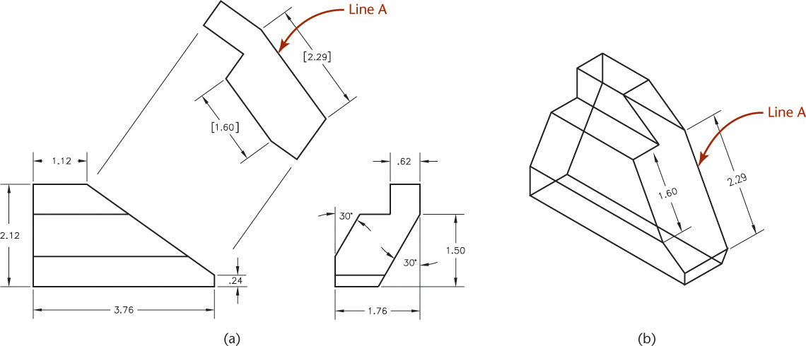
5.17 (a) The 2D CAD drawing displays the true length of line A in an auxiliary view. (b) The length of the line in the 3D wireframe model can be determined directly from the model.
Surface Models
CAD surface models define a shape by storing its surface information. A surface model is similar to an empty box. The outer surfaces of the part are defined (although unlike an actual box, these surfaces do not have any material thickness). Because the surfaces are defined, they can be shaded to provide a realistic appearance.
Surface modelers are traditionally used by industrial designers and stylists who create the outside envelope for a device. These designers need modeling tools that convey a realistic image of the final product. Software tools developed for their use focused first on the challenge of modeling the exterior of the product, not the mechanical workings within. Many surface modelers offer specialized tools for lighting and rendering a model, so designers can create photorealistic images that cannot be distinguished from the actual product (see Figure 5.18).
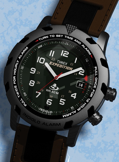
5.18 A Rendered Surface Model. The industrial designer for the Timex TurnAndPull alarm was concerned that the inner rings would look too deep or too busy. A rendered surface model allowed team members to see how it would look when manufactured. (Courtesy of Timex Group USA, Inc.)
Concurrent engineering and the use of the 3D CAD database as the product description contributed to the development of modeling software that satisfies the aesthetic needs of industrial designers as well as the functional information needed by engineers. Understanding surface modeling techniques will help you assess the kinds of features that are available in your modeler—and whether a dedicated surface modeler is required.
Surface Information in the Database
Most surface modeling software stores a list of a part’s vertices and how they connect to form edges in the CAD database. The surfaces between them are generated mathematically from the lines, curves, and points that define them. Some surface modelers store additional information to indicate which is the inside and which is the outside of the surface. This is often done by storing a surface normal, a directional line perpendicular to the outside of the surface. This allows the model to be shaded and rendered more easily.
Storing the definitions of the surfaces in the CAD digital database is termed boundary representation (BREP), meaning that the information contained in the database represents the external boundaries of the surfaces making up the 3D model. Remember that these surfaces have no thickness.
The following are basic methods used to create surface models:
• Extrusion and revolution
• Meshes
• Spline approximations
Extruded and Revolved Surfaces
You can define a surface by a 2D shape or profile and the path along which it is revolved or extruded.
Figure 5.19 shows a surface model created by revolution, and the profile and axis of revolution used to generate it. Regular geometric entities can be revolved or extruded to create surface primitives such as cones, cylinders, and planes. Surface primitives are sometimes built into surface modeling software to be used as building blocks for complex shapes.

5.19 Revolved Surface. The surface model in (a) was created by revolving the profile about the axis shown in (b).
Meshes
Mesh surfaces are defined by the 3D location of each vertex stored in the CAD database. Each group of vertices is used to define a flat plane surface. Figure 5.20 shows a mesh surface and a list of some of its vertices.
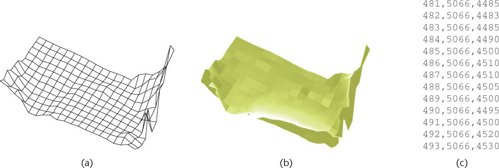
5.20 A Mesh Surface. A mesh surface is composed of a series of planar surfaces defined by a matrix of vertices, as shown in (c). The wireframe view of the mesh in (a) appears more like a surface in the rendered view shown in (b).
Some mesh surfaces are called triangulated irregular networks (TINs), because they connect sets of three vertices with triangular faces to serve as the surface model. A mesh surface can be useful for modeling uneven surfaces, such as terrain, where a completely smooth surface is not necessary. A sufficiently large matrix will result in correspondingly smaller triangles that can better approximate a smooth surface. Refining the mesh will produce a smoother surface, but the size of the CAD file will increase and result in slower software performance. Some modeling packages allow you to define a smoothed representation of the surface instead of the somewhat bumpy appearance of a strictly mesh surface.
NURBS-Based Surfaces
The mathematics of nonuniform rational B-spline (NURBS) curves underlies the method used to create surfaces in most surface modeling systems. A NURBS surface is defined by a set of vertices in 3D space that are used to define a smooth surface mathematically.
Rational curves and surfaces have the advantage that they can be used to generate not only free-form curves but also analytical forms such as arcs, lines, cylinders, and planes. This is an advantage for surface modelers that use NURBS techniques, as the database does not need to accommodate different techniques for surfaces created using a surface primitive, mesh, extrusion, or revolution.
Spline curves can be used as input for revolved and extruded surfaces that can be lofted or swept. Lofting is the term used to describe a surface fit to a series of curves that do not cross each other. Sweeping creates a surface by sweeping a curve or cross section along one or more “paths.” In both cases, the surface blends from the shape of one curve to the next (see Figure 5.21).
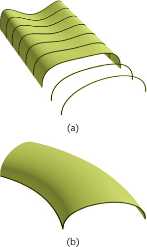
5.21 Lofting. A lofted surface (a) blends a series of curves that do not intersect into a smooth surface. A swept surface (b) sweeps a curve along a curved path and blends the influence of both into a smooth surface model.
NURBS surfaces can also be created by meshing curves that run perpendicular to each other, as illustrated in Figure 5.22.

5.22 When the spline curves shown here are used to generate a NURBS surface, the functions defining each curve are blended. (Courtesy of Robert Mesaros.)
Spotlight: Visible Embryo Heart Model
By modeling embryonic hearts at different stages, researchers were able to use the models to examine the way different tissue layers expand and move as the heart develops. To study blood flow in developing hearts that are only 0.8 millimeter across, Kent Thornburg and Jeffrey Pentecost created models from which they generated a 5-centimeter-wide stereolithography physical model.
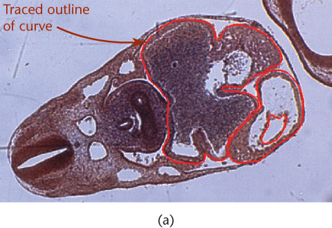
(a) Using cross sections of embryos from the Carnegie Collection of Human Embryos, the team made digital photomicrographs of each slide. Using the computer, they traced the outlines of heart tissues at each level.

(b) Lofting combined the cross sections into a surface model of the heart, shown in wireframe.
(c) The model made by stereolithography.
(Images courtesy of Dr. Jeffrey O. Pentecost, Director, Visible Embryo Heart Project, and Dr. Kent Thornburg, Director, Congenital Heart Research Center, at Oregon Health Sciences University, with the cooperation of Alias Wavefront and Silicon Graphics, Inc.)
Reverse Engineering
Most reverse engineering software traces a physical object to generate mesh data, or data points for a surface model. Points on the object are captured as vertices, then translated into a digital surface representation. Reverse engineering can be an easy way to capture the surface definition of an existing model. Designers might use traditional surface sculpting methods and then digitize the physical model to create a digital database. An existing part might be reverse engineered so that it can be added to the CAD database (Figure 5.23 shows data for the surface model in Figure 5.24 being created using a reverse engineering process.)

5.23 Digitizing a Model. A coordinate measuring system was used to digitize the clay model of the Romulus Predator. Seventeen hundred data points were captured by digitizing half of the quarter-scale clay model of the Predator. Digitizing the data and mirroring it in the model ensured side-to-side symmetry. (Courtesy of Mark Gerisch.)
5.24 Surface Patches. The lines on the surface model of the Predator prototype indicate individual surface patches that make up the model. Areas of the car with drastic curvature changes are divided into smaller patches, which keeps the mathematical order of the patches lower and reduces the overall complexity of the surface. (Courtesy of Mark Gerisch.)
Complex Surfaces/Combining Surfaces
To create a surface model, you do not create the entire surface at once—just patches to combine into a continuous model. Just as curves can be made of individual segments that are smoothed into a continuous curve, surfaces can be made of entities referred to as patches. Like a spline curve, a patch can be interpolated, or approximated.
A Coon’s patch is a simple interpolated surface that is bounded by four curves. Mathematical methods interpolate the points on the four boundary curves to determine the vertices of the resulting patch (see Figure 5.25).
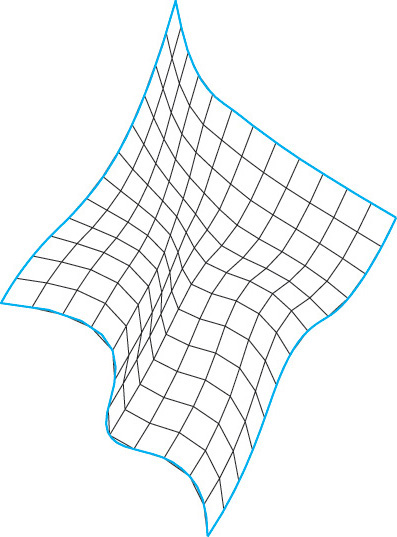
5.25 Coon’s Patch. The lines between the boundary curves in this Coon’s patch surface represent the shape of the surface and illustrate the influence of the boundary curves on the interpolated surface between them.
Surface patches are joined by blending the edges of the patches. Areas created by blending, or the surfaces created by fillets, corners, or offsets, are called derived surfaces. They are defined by mathematical methods that combine the edges of the patches to create a smooth joint.
Sometimes, complex surface patches are created by trimming. For example, a circular patch may start with a rectangular patch, then be trimmed to a circle, and finally be blended with other surface patches.
Some surface modeling systems include the use of Boolean operations, whereas others do not. Systems that do not include Boolean operations or good tools for trimming surfaces can be difficult to use to create a feature such as a round hole through a curved surface because the exact shape of the surface, including the hole, must be defined by specifying its edges.
Editing Surfaces
Once a surface has been defined, editing depends on the method used by the surface modeler to create and store the surface. Usually, the information describing the locations of vertices is editable, and each vertex can be changed. If the surface modeling software retains the original 2D profile that was extruded or revolved to produce the surface, it can be used to facilitate changes to these surfaces. If not, it can be difficult to efficiently edit the surfaces.
For NURBS surfaces, each control point can be edited to produce local changes in the surface model. (Editing Bezier surfaces, by the same token, produces global changes to the surface.) Grabbing and relocating vertices is a highly intuitive way to edit a surface model that contributes to its usefulness in refinement. The term “tweaking” is used to describe editing a model by adjusting control points individually to see the result. For example, the NURBS surfaces used to define the shape of the Predator’s exterior made it easy to use the surface model to explore design options in several areas (Figure 5.26).
5.26 The roof scoop on the Predator’s clay model was not visible enough, so the designer adjusted the control points in the surface model in real time until the scoop looked just right on screen. (Courtesy of Mark Gerisch.)
Surface Model Accuracy
Surface model information can be stored with more or less accuracy. Compare the meshes shown in Figure 5.27. The mesh at left contains fewer vertices than the mesh shown in 5.27b. Although the surface shown in 5.27b is more accurate, the additional information makes its file size larger. This requires more computer processing to store and interact with the model. Depending on your purpose, the smaller number of vertices may be satisfactory.
5.27 Accuracy and Surface Mesh. The mesh in (a) has fewer vertices and larger facets than the mesh used in (b). The finer mesh in (b) more accurately represents the cylindrical shape of the bolt.
Surface models used for computer-aided manufacturing (CAM) require a high degree of accuracy to produce smooth surfaces. The trade-off between speed and accuracy may be resolved by setting the surface display to a less accurate faceted representation and storing a smoothed or more highly defined surface definition in the database. It is important to distinguish between the screen display of the model and the surface definition stored in the database.
Splines used to create surfaces can also vary in accuracy. Splines can have more or fewer control points that you can use to shape the surface. To model surfaces smoothly, fewer control points may allow more fluid curves. A mesh surface used to calculate area may not be as accurate as one created using a smoothing algorithm such as NURBS or Bezier.
Tessellation lines are used to indicate surfaces in a wireframe view, and they may or may not reflect the accuracy of the surface (see Figure 5.28). It is important to distinguish when tessellation lines represent the accuracy of the view of the model, and when they represent the accuracy of the model stored in the database. If the software accurately represents the actual geometry of the model in the model database, the tessellations simply represent the model in the on-screen view.
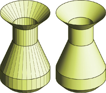
5.28 Tesselation Lines. The faceted representation on the left uses planar surfaces to approximate smooth curves.
Using Surface Models
The primary strength of a surface model is improved appearance of surfaces and the ability to convey these complex definitions for computer-aided manufacturing. Customers purchase products not only on their function but also on their styling. A realistically shaded model can be used with potential customers to determine their reactions to its appearance. Lighting and different materials can be applied in most surface modeling software to create very realistic looking results (Figure 5.29). Many consumer products often start with the surface model, then the interior parts are engineered to fit the shape of the styled exterior. When surface models can be used in place of a physical prototype—or in place of the product itself for promotional purposes—the savings add to their cost effectiveness.
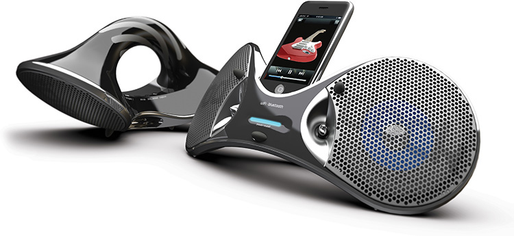
5.29 This docking station illustrates the complex curves possible in a surface model. (Image courtesy of ©2016 Dassault Systèmes SolidWorks Corporation.)
Because the relative locations of surfaces from a particular direction of sight can be calculated, surface modeling systems can automatically remove back edges (or represent them as hidden lines). Surface definitions remove the ambiguity inherent in some wireframe models and allow you to see holes and front surfaces by hiding the nonvisible parts of the model.
The complex surfaces defined by a surface model can be exported to numerically controlled machines, making it possible to manufacture irregular shapes that would be difficult to document consistently in 2D views. Both surface and solid models can be used to check for fit and interference before the product is manufactured. Often, surface models can be converted to solid models and vice versa.
Because surface models define surfaces, they can often report the surface area of a part. This information can be useful in calculating heat transfer rates, for example, and can save time, particularly when the surface is complex. The accuracy of the calculations may depend on the method used by the software to store the surface data.
Complex surfaces can be difficult to model. The cost-effectiveness of surface modeling depends on the difficulty of the surface, the accuracy required, and the purpose for which the model will be used. Many modeling software systems offer a combination of wireframe, surface, and solid modeling capabilities, making it possible to weigh the benefits against the difficulties and the time required to create each type of model.
Solid Models
Solid models go beyond surface models to store information about the volume contained inside the object. They store the vertex and edge information of the 3D wireframe modeler, the surface definitions of the surface modeler, plus volume information. Many solid modelers also store the operations used to create features, which makes it possible to edit them quickly (see Figures 5.30 and 5.31). Solid models closely approximate physical models, making them especially useful for defining, testing, and refining the designs they represent.
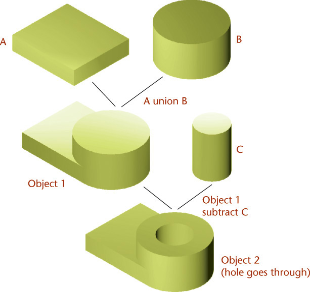
5.30 Order Matters. The order of operations matters when you use Boolean operations to create a solid model—and when you edit it (see Figure 5.31).
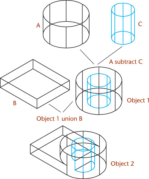
5.31 Joining A and B after the hole is created by subtracting C changes the design—the hole no longer goes through the entire part.
Tip
Understanding basic modeling methods will help you assess the modeling software of tomorrow. Some new modelers, referred to as “direct” or “explicit” modelers, such as Creo and SpaceClaim, offer a broad command set that adopts features from traditional surface and solid modelers.
Using 3D Solid Models
Many of the examples so far illustrated how accurate representation of a 3D object provides valuable engineering information. Solid models are highly visual and easy to understand and measure. They are also highly accurate if modeled accurately. Solid models are often able to replace physical models, as well as control CAM equipment, which adds to their cost-effectiveness.
In addition, 3D solid models are particularly suited for use with analysis packages. They contain all the information about an object’s volume, and volume is important to many engineering calculations. Mass properties, centroid, moments of inertia, and weight can be calculated from the solid model as often as needed during the refinement process. The system behavior can be simulated from the wealth of information available in the model.
Solid models provide information needed for other analyses. Finite element analysis (FEA) methods break up a complex object into smaller shapes to make stress, strain, and heat transfer easier to calculate. Because the solid model defines the entire object, FEA software can use this information to generate an FEA mesh automatically for a part. This allows inclusion of this type of analysis earlier in the design process, incorporation of changes, and testing of the new model with FEA analysis again. Some FEA and solid modeling packages are integrated to provide this analysis within the modeling software. Others even allow direct model optimization based on the FEA results, creating a new version of the model that the designer can then revise further.
5.4 Constraint-Based Modeling
Constraint-based modeling has several advantages for engineering design. As the design evolves, constraint-based models can be updated by changing the sizes and relationships that define the model. In traditional solid modeling methods, changing the size of one feature may require several others to be changed, or the model may need to be totally re-created. Because of the iterative nature of the design process, a design is repeatedly modified as it is refined. The model’s responsiveness can result in more cycles during the refinement stage (or more cycles in less time) and, ultimately, a better design.
Neptune Seatech Oy made the decision to switch from a 2D design method to a constraint-based 3D modeler, SolidWorks, so it could get its products to market faster while preserving the iterations needed for complex, accurate designs. Neptune Seatech is a Finnish engineering company that specializes in the design of vehicles for subsea applications—passenger and research submarines. To meet increasingly rigorous design, performance, and safety standards, the company found 2D methods made it hard to complete the desired number of design iterations and still meet product development deadlines. Its first project using the constraint-based 3D modeler, a floating bridge for ferries, took only 18 weeks to produce (see Figure 5.32).
5.32 Neptune Seatech’s parametric model of the floating bridge for ferries was modified to create a family of designs for the variations in ferry landings. (Courtesy of Neptune Seatech Oy.)
The company enjoyed two other benefits of constraint-based modeling. First, the ease with which constraint-based models can be updated makes it possible to create families of designs. Neptune’s floating bridge allows cars to pass from the ferry to land and vice versa during loading and unloading. Because each landing site is slightly different, the main dimensions of a given bridge vary slightly from one site to another. The bridge manufacturer that hired Neptune had several designs previously created for specific landing sites. To eliminate confusion in manufacturing, the customer wanted a design that could be updated for new bridges. Neptune proposed to design one bridge, then produce the others by changing the length and width factors. The constraint-based model of the bridge made it easy to change the pertinent dimensions and have the software update the related parts to a new size. The investment in the bridge model was used to refine the original bridge design, then used again as a starting point for variations in the product family (see Figure 5.33).

5.33 Neptune Seatech’s bridge model, created in SolidWorks, involved more than 1700 parts. (Courtesy of Neptune Seatech Oy.)
Neptune also enjoyed the software’s ability to analyze mass properties. The weight and volume data for a floating bridge need to be evaluated during design so that the resulting bridge floats at the correct level. Calculating the weight of a floating bridge design would have taken 1 to 2 weeks using Neptune’s previous methods, but the built-in capabilities of SolidWorks made it possible to monitor this data throughout the design process. The ease with which the model could be modified made it possible to analyze the model, make changes, and analyze the model again. The software also made it possible for analysis to occur earlier in the design process, allowing more time to optimize the design.
Constraint-based modeling also improves designs by focusing the modeler on the design intent for the product. If a constraint-based model is to be updated successfully when changes are made, the rules for building the model must capture the intended design solution for the system or device. The extra attention and planning required to capture design intent in the model makes the designer carefully consider the function and purpose of the item being designed, which in turn results in better designs.
5.5 Constraints Define the Geometry
In a constraint-based model, an object’s features are defined by sizes and geometric relationships stored in the model and used to generate the part. Two basic kinds of constraints are used to drive the model geometry.
• Size constraints are the dimensions that define the model. The choice of dimensions and their placement is an important aspect of capturing the design intent.
• Geometric constraints define and maintain the geometric properties of an object, such as tangency, verticality, and so on. These geometric constraints are equally important in capturing design intent.
In constraint-based modeling, a parameter is a named quantity whose value can change; it is similar to a variable. Like a variable, a parameter can be used to define other parameters. If the length of a part is always twice the width, you can define its size as “2 × Width,” where Width is the name of the dimension.
Unlike a variable, a parameter is never abstract: it always has a value assigned to it, so that the model can be represented. For example, the parameter Width is defined by a value, such as 3.5. The value for the length parameter is calculated based on the Width, so in this case Length is 7. If the width value is changed to 5, the length is automatically updated to the new value of “Width * 2,” or 10 (see Figure 5.34).

Even something as simple as this rectangular block may have design intent built into its model. As it is being updated, do you want the center of the part to stay fixed and the part to elongate in both directions, or do you want it to lengthen all in one direction? If so which end should stay put?
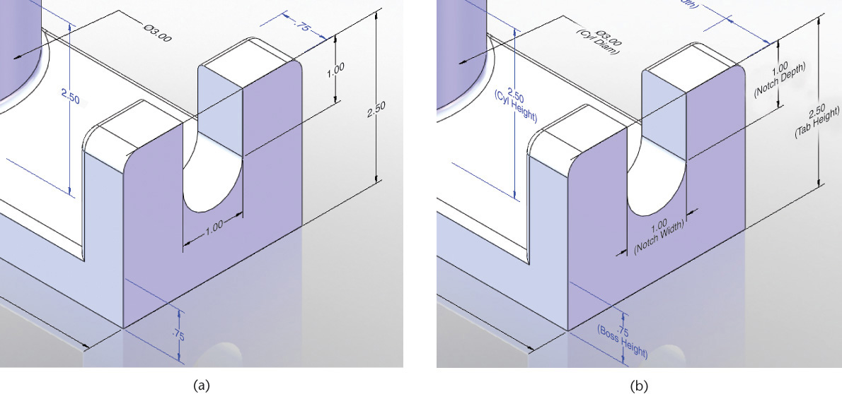
Figure 5.35 shows a part that has been modeled in a 3D constraint-based design package. The parameters driving the geometry of the model are indicated on the drawing. When the parameter value for the length of the part was changed, the part was updated automatically, as shown in part b of the figure. Notice that the threaded length did not increase. If you wanted the thread length to increase as the bolt was lengthened, you would need to define the constraints and parameters differently.

5.35 When the length dimension increased to .750, the part was updated to reflect this new size constraint. Notice that the threaded length remained the same and the bolt head remained attached after the update. The modeler maintained the size and geometric relationships that were defined.
Dimensions in a constraint-based model can behave in different ways. A dimension can be:
• A size constraint: changing the dimension value updates the model feature. These are often called driving dimensions.
• A parameter used in an equation that “drives” the size of a model feature.
• A reference dimension, which gets its value from the model geometry, but is not a size constraint for the model. These are often called driven dimensions.
• A dimension that is purely a text note on a drawing or model view and whose value may not relate to the model geometry.
• A combination of the above.
Driving Dimensions
Driving dimensions control the size of a feature element in the model. Each driving dimension has two components: its name and its numerical value. Naming the dimensions allows them to be used in equations or relations that define other parts of the model geometry. The numerical value may be entered as a number in the definition of the dimension, or it may be derived from an equation. Figure 5.36a shows the shaft support part with its dimension values displayed; Figure 5.36b shows the same part with the dimension names. The constraint-based modeling software allows you to switch between display of numeric and named dimensions in your model. Some modelers also allow you to show the dimensions so that they reveal the formulas used to relate dimensions to one another.
5.36 Two Ways to Display Dimensions in the Constraint-Based Model. (a) The numerical display shows the current value for the dimensions. (b) Showing the parameter name can help you locate dimension names to be used in the dimension for another entity.
Formulas in Dimensions
Like the geometric constraints in the model, the size parameters create relationships between features of the part that can be captured in formulas. For example, if you wanted to maintain a constant material thickness around the outside of a central hole with diameter d2, you could enter the equation d1 = d2 + 1.00 for the diameter of the outer cylinder. Doing so, ensures that the driven dimension (d1) will be 1.00 overall more than d2 no matter what value is entered for d2.
Another example is adding four holes to a rectangular base plate that should be centered 0.75 inch away from the edge of the plate. If the width of the plate changes, the hole locations should also. Defining the location of the holes using the equation h_location = width/2 – .75, where width is the plate’s width dimension and h_location is given from the center of the part, will make the holes stay in the same relative positions. To change the distance from the edge from .75 to 1.00, you would just update the equation and regenerate the model.
Equations in constraint-based dimensions generally use operators similar to those used in a spreadsheet or other programming notation. Many modelers make it easy to import to and export dimension values from an outside application, such as a spreadsheet. Complex formulas can be used to calculate sizes in the spreadsheet or other program, and the resulting values can be imported back into the modeling package. Each modeling package has its own notation and syntax. Table 5.1 lists operators that can be used in equations in SolidWorks. Most modelers have a similar list.
Operator |
Name |
Notes |
+ |
plus sign |
addition |
– |
minus sign |
subtraction |
* |
asterisk |
multiplication |
/ |
forward slash |
division |
^ |
caret |
exponentiation |
sin (a) |
sine |
a is the angle; returns the sine ratio |
cos (a) |
cosine |
a is the angle; returns the cosine ratio |
tan (a) |
tangent |
a is the angle; returns the tangent ratio |
sec (a) |
secant |
a is the angle; returns the secant ratio |
cosec (a) |
cosecant |
a is the angle; returns the cosecant ratio |
cotan (a) |
cotangent |
a is the angle; returns the cotangent ratio |
arcsin (a) |
inverse sine |
a is the sine ratio; returns the angle |
arccos (a) |
inverse cosine |
a is the cosine ratio; returns the angle |
atn (a) |
inverse |
a is the tangent ratio; returns the angle |
arcsec (a) |
inverse |
a is the secant ratio; returns the angle |
arccosec (a) |
inverse cosecant |
a is the cosecant ratio; returns the angle |
arccotan (a) |
inverse cotangent |
a is the cotangent ratio; returns the angle |
abs (a) |
absolute value |
returns the absolute value of a |
exp (n) |
exponential |
returns e raised to the power of n |
log (a) |
logarithmic |
returns the natural log of a to the base e |
sqr (a) |
square root |
returns the square root of a |
int (a) |
integer |
returns a as an integer |
sgn (a) |
sign |
returns the sign of a as –1 or 1; For example: sgn (–21) returns –1 |
pi |
pi |
ratio of the circumference to the diameter of a circle (3.14...) |
It is important to keep track of the relationships you create. Most software allows you to name and document your constraint-based dimensions so you (and your colleagues) can interpret parameter names more readily. The software will generate a name for each dimension by default, but you should give key dimensions recognizable names so they are easier to interpret.
Parameters that are common to more than one part in an assembly are called global parameters. Naming global parameters that can be used throughout an assembly is a powerful means of ensuring that parts work together and that critical dimensions are updated in all parts of an assembly. With global parameters, it is even more important to choose names that are clear and to document their purpose in the notes field.
Driven and Cosmetic Dimensions
Driven or reference dimensions are associated with the model geometry but are not used to create the constraint-based model. Sometimes it is necessary to add a dimension to a drawing that was not needed to create the model. A driven dimension is a one-way link from the database; it cannot be used to change the model, but it will be updated if the model changes.
A cosmetic dimension has no link to the model; it is simply a text label. To dimension a feature at a size different from what is in the model, you must use a cosmetic dimension or otherwise break the link to the database value for the feature.
You should not often need driven dimensions. A well-created constraint-based model contains all the dimensional relationships needed.
Using the shaft support as an example again, a relationship can be defined so the diameter of the hole is always 1 inch smaller than the diameter of the cylinder. Changing the size of the cylinder will cause the diameter of the hole to change to preserve the size relationship.
Feature-Based Modeling
Constraint-based modeling is also called feature-based modeling because its models are combinations of features. Creating a constraint-based model is similar to creating any other solid model. However, in constraint-based modeling the resulting part is derived from the dimensions and constraints that define the geometry of the features. Each time a change is made, the part is re-created from these definitions. Individual features and their relationships to one another make up the constraint-based model.
A feature is the basic unit of a constraint-based solid model. Each feature has properties that define it. When you create a feature, you specify the geometric constraints that apply to it, then specify the size parameters. The modeler stores these properties and uses them to generate the feature. If an element of the feature, or a related part of the model, changes, the modeling software regenerates the feature in accordance with the defining properties assigned to it. For example, an edge that is defined to be tangent to an arc will move to preserve the tangency constraint if the size of the arc is changed.
Some features, such as holes and fillets, may use predefined features with additional properties that are maintained as the model is updated. For example, a “through hole” (one that goes completely through the part feature) will be extended if the part thickness increases.
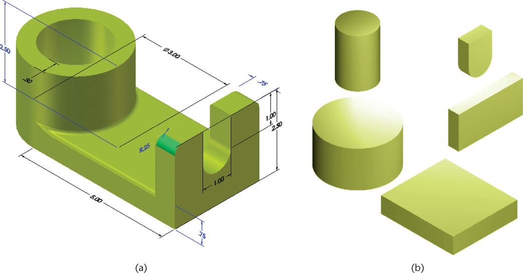
When you look at the fixed-height shaft support shown in Figure 5.37a, can you identify the features that make up its shape? Figure 5.37b shows the major cylinder, hole, plate, end plate, slot, and rounds that form the model of the shaft support.
Being able to update models easily to reflect changes in the design is a key ability of constraint-based modelers. If you are not using a constraint-based solid modeling program, you may have to re-create the feature just to change a size. This can result in considerable time and effort, especially for interrelated features.
In addition to defining relationships between features, constraint-based modeling software also allows you to use constraints and parameters across parts in an assembly. Thus, when a part changes, any related parts in the assembly can also be updated. Because the software regenerates the features and parts from the relationships stored in the database (see Figure 5.38), planning constraint-based relationships that reflect the design intent of the part or product is the key to efficient and useful constraint-based models.

5.38 Model Tree. The window at the left side of the screen called the “model tree” (enlarged here) lists the features in the order in which they were created. The icon next to the feature indicates the operation used to create the feature. Extrusions and extruded cuts were used to form the cylinder, baseplate, and hole. Then, the end feature was extruded and the slot created using an extruded cut. Finally, fillets were added to round the edges.
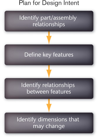
5.6 Planning Parts for Design Flexibility
Design intent refers to the key dimensions and relationships that must be met by the part. Where does the part need to fit into other parts? Do certain features need to align with other features? How will the part change as the design evolves? By thinking about these relationships, you can organize the features so that the structure of the part and its relationships are the foundation for later features. Four key aspects of planning for design intent are summarized in Figure 5.39. Of course, you cannot know everything about a design before you begin, and there will be changes that will require more work than others; but starting your model with the geometric relationships in the design in mind will allow you to benefit from the power of constraint-based modeling. To see how a constraint-based model can reflect design intent, you should understand some basics about constraint-based modeling software.
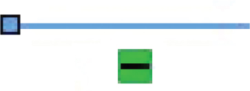
Constraint-based modeling software in many ways parallels the design process. To start creating a part, you often start with a 2D sketch of the key shape of a feature, such as that shown in Figure 5.40. The initial sketch may be rough in appearance because the software will apply constraints to define the relationships between the simple 2D geometric elements of your sketch. This process is similar to the way one of your engineering colleagues interprets your hand-drawn sketches. If lines appear to be perpendicular or nearly so, your colleague assumes that you mean them to be perpendicular, without your having to mark the angular dimension between the lines. In a similar way, constraint-based modelers apply constraints to your rough sketch, so that lines that appear nearly perpendicular, parallel, vertical, horizontal, concentric, or collinear will have a constraint relationship added to them so that they function that way in the model. This process is called “solving” the sketch in some modeling software, because the software is interpreting and assigning dimensions and constraints to generate a 2D “profile” of the feature. Before you generate the actual feature, you can review and change the dimensions and geometric constraints so they are what you intended. This step is key to defining your design intent. The sketch constraints in Figure 5.40 have already been added.

5.40 A constrained sketch is used as the basis for a model feature. Geometric constraints are identified by the blue symbols.
To generate a 3D feature, you then select a command to extrude, revolve, sweep, or blend the profile geometry. Figure 5.41 shows the profile in Figure 5.40 as it would appear after being (a) extruded, (b) swept, (c) revolved, and (d) lofted to create different types of features from the 2D sketch.
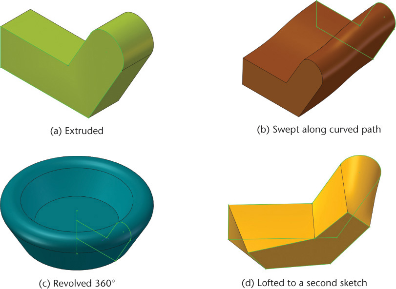
5.41 Same Sketch, Different Operations. The same sketch was used to create each of these features. The sketch in (a) was extruded, in (b) swept along a curved path, in (c) revolved 360° about an axis, and in (d) lofted between the sketch and a second sketch with angled lines and a straight top.
5.7 Sketch Constraints
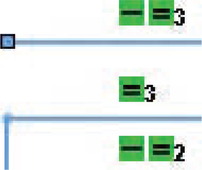
Constraint-based modeling software starts by automatically interpreting your sketch, to define the constraints that it will hold constant. To do so, it evaluates your sketch against a set of rules stored in the software. A line, for example, that is drawn within 3° or 4° of being horizontal will be constrained to remain horizontal. Your sketch will be altered so the line you drew is, in fact, horizontal. The software will apply the constraints it needs to solve the sketch.
Constraint-based modeling programs allow you to review the constraints that are applied to the sketch geometry so you can change them to those needed to reflect your design intent. Table 5.2 describes some possible sketch constraints and shows symbols often used to indicate them on screen. (Different modelers use different symbols and means of displaying the constraints—see Table 5.3 and Figure 5.42). These constraints may create relationships to other lines in the sketch or to geometry in an existing feature.
Constraint |
Rule |
Symbol |
Horizontal |
Lines that are close to horizontal are constrained to be horizontal (usually you can control the number of degrees for this assumption, typically set to 3° or 4°). |
H |
Vertical |
Lines that are close to vertical are constrained to be vertical (usually within 3° or 4°). |
V |
Equal length |
Line segments that appear equal length are constrained to be equal. |
L1, L2, etc. |
Perpendicular |
Lines that appear close to 90° apart are constrained to be perpendicular. |
⊥ |
Parallel |
Lines that appear close to parallel are constrained to be parallel. |
// |
Collinear |
Lines that nearly overlap along the same line are assumed to be collinear. |
No symbol displayed |
Connected |
Endpoints of lines that lie close together are assumed to connect. |
Dot located at intersection |
Equal coordinates |
Endpoints and centers of arcs or circles that appear to be aligned horizontally or vertically will be constrained to have equal X- or equal Y-coordinates. |
Small thick dashes between the points |
Tangent entities |
Entities that appear nearly tangent are constrained to be tangent. |
T |
Concentric |
Arcs or circles that appear nearly concentric are concentric. |
Dot at shared center point |
Equal radii |
Arcs or circles that appear to have similar radii are constrained to have equal radii. |
R |
Points coincide |
Points sketched to nearly coincide with another entity are assumed to coincide. |
No symbol displayed |
Table 5.3 Selected Constraint Relations in SolidWorks
$$$$$Symbol |
Relation |
Entities to Select |
Result |
|
Horizontal or Vertical |
One or more lines or two or more points |
The lines become horizontal or vertical (as defined by the current sketch space). Points are aligned horizontally or vertically. |
|
Collinear |
Two or more lines |
The items lie on the same infinite line. |
Coradial |
Two or more arcs |
Items share the same center point and radius. |
|
|
Perpendicular |
Two lines |
The two items are perpendicular to each other. |
|
Parallel |
Two or more lines. A line and a plane (or a planar face) in a 3D sketch |
The items are parallel to each other. The line is parallel to the selected plane. |
ParallelYZ or ParallelZX |
A line and a plane (or a planar face) in a 3D sketch |
The line is parallel to the YZ (or ZX) plane with respect to the selected plane. |
|
|
Tangent |
An arc, ellipse, or spline, and a line or arc |
The two items remain tangent. |
|
Concentric |
Two or more arcs, or a point and an arc |
The arcs share the same center point. |
Midpoint |
Two lines or a point and a line |
The point remains at the midpoint of the line. |
|
|
Intersection |
Two lines and one point |
The point remains at the intersection of the lines. |
Coincident |
A point and a line, arc, or ellipse |
The point lies on the line, arc, or ellipse. |
|
|
Equal |
Two or more lines or two or more arcs |
The line lengths or radii remain equal. |
Symmetric |
A centerline and two points, lines, arcs, or ellipses |
The items remain equidistant from the centerline, on a line perpendicular to the centerline. |


5.42 Changing Constraint Defaults. The Constraint Settings dialog box in AutoCAD lets you change the priority in which the constraints are applied. You can also set the tolerance for sketched endpoints to be considered coincident, and lines to be assumed horizontal or vertical. Understanding which assumptions are being applied to your sketch can help you define the exact geometry you require. (Autodesk screen shots reprinted courtesy of Autodesk, Inc.)
Step by Step: Constraining a Sketch
Like a hand-drawn sketch, the sketch for a constraint-based model captures the basic geometry of the feature as it would appear in a 2D view.
![]() Sketch the basic shapes as you would see them in a 2D view. Many modelers will automatically constrain the sketch as you draw unless you turn this setting off in the software.
Sketch the basic shapes as you would see them in a 2D view. Many modelers will automatically constrain the sketch as you draw unless you turn this setting off in the software.

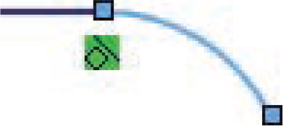
![]() Apply geometric constraints to define the geometry of the sketch. If it is important to your design intent that lines remain parallel, add that constraint. If arcs must remain tangent to lines, apply that constraint. Here, lines A and B have been defined to be parallel; note the parallel constraint symbol.
Apply geometric constraints to define the geometry of the sketch. If it is important to your design intent that lines remain parallel, add that constraint. If arcs must remain tangent to lines, apply that constraint. Here, lines A and B have been defined to be parallel; note the parallel constraint symbol.

![]() Add dimensional constraints. The length of line B was sketched so that the software interpreted the dimensional constraint to be 3.34. The designer changed this dimension to 3.75 (the desired length), and the length of the line was updated to the new length.
Add dimensional constraints. The length of line B was sketched so that the software interpreted the dimensional constraint to be 3.34. The designer changed this dimension to 3.75 (the desired length), and the length of the line was updated to the new length.

Tip
It is often useful to start drawing the feature near the final size required. Otherwise if the software is automatically constraining your sketch, a line segment that is proportionately much shorter may become hard to see or even considered effectively zero length and deleted by the software.
Not all constraint-based modeling programs apply all these constraints, nor do they apply them in the same fashion. Study the constraints available in the software you use and determine their effect on the sketch. You also may be able to set the threshold values for various constraints. For example, instead of having lines at 1° be automatically constrained as horizontal lines, you may wish to increase this value to 3° (Figure 5.42). If you are having difficulty getting the constraints you desire applied to the sketch, you may want to turn off automatic constraint application and select each specific constraint to apply to your sketch.
Most constraint-based modeling programs let you remove or override a constraint that is applied, or specify that the geometry is exact as drawn. Sometimes, you may have to force the sketch closer to the desired relationship. For example, if two lines are too far off in the sketch to be constrained as perpendicular by the software, you could add an angular dimension of 90° between them to force them to that relationship. With the dimensions driving the geometry to the condition you want, the software may apply the perpendicular constraint. Once the constraint is applied, you often can delete the dimension you added.
It is usually beneficial to let geometric constraints determine much of your sketch geometry, then dimension the sizes and relationships that cannot be defined using constraints. You could use a constraint-based modeler as you would a solid modeler, adding dimension values to define all the features, but this would not build in the intelligence that allows the software to automate updating the model.
Overconstrained Sketches
Sketches used in constraint-based modeling may not be overconstrained. An overconstrained or overdimensioned sketch is one that has too many things controlling its geometry.
The sketch shown in Figure 5.43 is overconstrained. Because the top arc is constrained to be tangent to both vertical lines, and its radius is dimensioned (sd0), the width of the sketch is defined. The horizontal dimension shown at the bottom (sd2) defines this width again. If both the arc radius dimension and the overall width dimension were allowed in the model and one of them changed, it would be difficult or impossible for the part to be updated correctly. If the overall width changed and the tangent constraint or arc radius did not, the sketch geometry would be impossible.

Underconstrained Sketches
An underconstrained or underdimensioned sketch is one that has too few dimensions or constraints and is therefore not fully defined.
The sketch shown in Figure 5.44 is underconstrained. It lacks a height dimension controlling its vertical size. Without this dimension the sketch is not fully defined. Some software will allow you to create a 3D feature from an underconstrained sketch as long as the sketch follows basic rules—for example, the sketch does not cross itself, and the sketch encloses an area. If the sketch is underconstrained, the software assumes values for unspecified dimensions based on the sizes drawn. This can be helpful when you are trying out ideas, but it is best to plan to create a model that reflects your design intent.
Dimensions can easily be changed by typing a new value, so go ahead and guess the size and change it later if needed; but keep in mind that choosing which dimensions to use to define the sketch is a critical aspect of making sketches and features that will be updated as expected when a dimension changes.
Applying Constraints
You should select dimensions that define the proper relationships between the sketched geometry and other existing features in your model. The surfaces between which you choose to create the dimensions are a large factor in creating a model that will be updated in the desired manner. You should not let the rules of your software package determine the dimensions, as it is unlikely that they will reflect your design intent.
When you are dimensioning a sketch used to create a feature, place the dimensions where you can view them clearly. Later, if you create a drawing from your model, you will be able to clean up the appearance of the dimensions if needed. You can move dimensions, change their placement, and arrange them so they follow the standard practices. Good placement practices such as placing dimensions outside the object outline and keeping the dimensions a reasonable distance from one another will make the dimensions in your model easier to read.
3D models are accepted as final design documentation. When you are going to use the model as the design database and not provide drawings, it is even more important to ensure that dimensions and tolerances shown in the model are clear. You will learn more about practices for documenting inside the 3D model in Chapter 11.
If you do a good job selecting the dimensions that control the drawing geometry, you will have little cleanup work to do later when you are creating drawing views.
Setting the Base Point
Some constraint-based modeling software assumes a base point in the sketch for the first feature you create. The base point is fixed on the coordinate system; the other sketch geometry is located on the coordinate system based on its relationship to this base point. The resulting feature will stay fixed on the coordinate system at this base point. When dimension values change, they will change relative to that point. There is only one base point per model.
The base point is indicated in Figure 5.45a by the × in the lower right corner of the sketch. When the width dimension changes, the sketch is updated to the new size while leaving the base point fixed on the coordinates. The rest of the sketch geometry is reoriented, as shown in Figure 5.45b.

5.45 Base Point. The base point fixes the sketch on the coordinate system in this underconstrained sketch. The base point serves as a fixed point when the model is updated. In AutoCAD, adding a Fixed Point constraint lets you identify the base point; otherwise, it is determined by software rules.
If your software uses a base point, it should become the base point for the entire model. When the model is updated, all dimensions will be updated from this point. A good rule of thumb is to identify a fixed point on your model that you would use as a starting point for measuring the part for inspection purposes. Use this point as the base point, or locate your dimensions from it as if it were the base point.
Locating most of your dimensions from a common edge or major surface can be effective for two reasons. First, it helps you create dimensions that will be useful for inspecting the part after manufacture; the dimension values in your model will measure from the same point that an inspector will use to measure the finished part. Second, it helps you anticipate how the model will be updated. When a value is changed, the features on the model will be updated (move) relative to the edge referenced in their dimensions. When you locate dimensions relative to other features you may have difficulty predicting how the model will be updated because you have to add the effect of changes to the intermediate features.
More important than any rule of thumb governing dimension selection or placement is to consider thoroughly the parts you are designing and to make the drawing geometry, constraints, and dimensions reflect the design intent for the part. In some cases, dimensioning a part from another feature is required to reflect the design intent. Figure 5.46 shows two sketches that have the same geometry but are dimensioned differently. When the 2.00 height dimension is changed to 2.50, how will each of these drawings be updated?
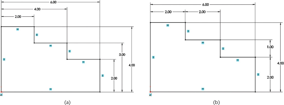
5.46 These two sketches of the same part have very different relations built into the dimensions for the sketch. The sketch in (a) relates all dimensions to the left and bottom edges of the part. The sketch in (b) has a chain of relationships built into the dimensions.
In the first case, shown in Figure 5.46a, the height of the 2.00 “step” will change to 2.50, narrowing the gap between it and the 3.00 step. In Figure 5.46b, the height of the 2.00 step will change to 2.50, and the height of the next step will be updated to 3.50 units so it remains 1.00 unit above it. In this case, the narrow gap will occur between the 3.50 and the 4.00 step. Either is correct to the extent that it reflects the intended design.
5.8 The Base Feature
To create useful relationships in a constraint-based model, it is helpful to start out your model with a good base feature. The base feature is the first feature you create. The other features are created using relationships that locate them to the base feature. Subsequent features are updated based on their relationships to the base feature or to one another. You should generally choose a fairly large, significant feature as the base feature.
Figure 5.47 shows the cylinder that could be created as the base feature for the shaft support and the other features that will relate to it. The major cylinder would make a good base feature because it is a significant feature of this part, and the other features make sense related to it. If the design intent of the part centers on the cylinder, its size and location determine the size and shape of other features. The width of the base plate will depend on the stability needed for the size of the cylinder. The hole for the shaft must be centered inside the cylinder and sized to leave enough remaining material for the wall thickness. Using the cylinder as the base feature also makes sense from the standpoint of the part’s role within a larger assembly, as its size could depend on the shaft being designed in a different part. By building your model around the major cylinder, you make it possible to update all features automatically if the cylinder size changes.
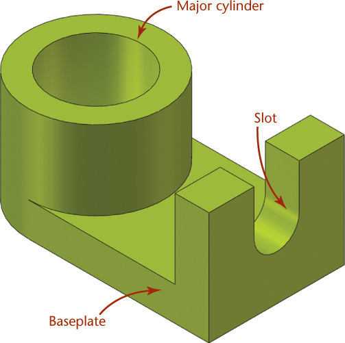
5.47 Base Feature. The major cylinder for the shaft support makes a good base feature because the cylindrical shaft to be supported is an important aspect of this design.
Adding Features to the Model
When you add features to the model, the way you constrain the sketch determines how it relates to the other features. Just as the base point serves to locate the base feature, at least one of the constraints applied to subsequent sketches must tell the software how the new feature relates to an existing feature.
To create the second feature, you can use a dimension to locate it relative to an existing edge or use a geometric constraint to align one of the sketch entities to the existing geometry. For example, you could dimension the center point of a hole to be a certain distance from the end of an existing feature or constrain the hole to be concentric to a cylinder or arc on an existing feature.
The way you dimension, constrain, or align your second feature determines how it will be updated with respect to the first feature. Use the things you know about the design to add features. Where are the fixed points on the model, and how does the feature you are adding relate to them? What are the conditions that the new feature needs to satisfy at all times? If existing features were to change, how would the feature you are adding need to change? In some cases, a simple dimension from an existing edge may be all that is needed to add the feature. In other cases, you will want to build in geometric or size relationships needed in the design. The basic process of constraint-based part modeling is illustrated in Figure 5.48. Starting with the base feature, you build a model by adding features and relating them to existing features. For each feature, the same basic process applies.
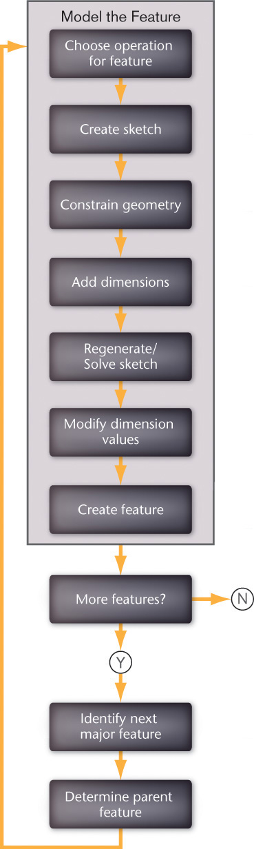
Spotlight: Use an Existing Edge
Pro/ENGINEER (as well as many other modelers) has a sketch command that allows you to specify an edge on an existing feature to project as a line in your sketch. This command creates the line in the sketch and constrains the sketched line to be collinear with the existing geometry in a single step. Even better, if the edge on the feature moves, the sketched entity moves with it to stay in alignment.
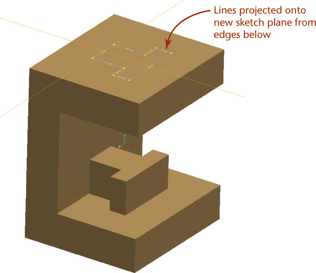
(Courtesy of Mark Perkins.)
Parent-Child Relationships
Constraint-based modeling software stores information about each feature and its relationship to its parent feature. The term parent-child relationship is used to describe how one feature is derived from another feature. This relationship is defined by the geometric constraints applied to the sketch as well as its dimensioned size constraints. Planning when creating a parent-child relationship is important.
The base feature is the parent feature for the next feature created from it. Just as real children depend on their parents, child features are dependent on their parent features. If a parent feature moves, the child feature moves in relation to it. For example, when the hole feature was added to the shaft support part, its location was defined as concentric with the major cylinder. When the cylinder’s location changes, the hole feature remains concentric with the cylinder (Figure 5.49). If the hole is located relative to the baseplate or to some other feature and the cylinder is moved, the hole will not move with it (Figure 5.50).

5.49 The hole is concentric with the cylinder. As the baseplate length increases, the hole remains concentric.

5.50 The hole dimensioned from the right end of the part is in the wrong location when the baseplate length changes.
If you delete a feature, you will also delete its child features unless you redefine them so that they are related to a different parent feature. This is another reason for selecting a good base feature; you do not want the first feature you create to be something that might be deleted later in the design. Not all features will have child features, but all features other than the base feature must be related to some parent feature.
One way to visualize the parent-child relationships as you plan your model is to build a tree diagram. The relationships in the Clamp Bottom model in Figure 5.51 are illustrated in the Parent/Child Relationships window. The panel labeled Children shows that the feature named Loop strap has Handlebar hole, Boss strain fillet, and Outer edge fillet as its children, along with the sketch that formed its cross-sectional shape. These features may or may not have children (or “grandchildren”) of their own. The panel labeled Parent shows that the parent features for Loop strap are Sketch4, the Front datum plane, the Screw boss feature, and the Origin of the coordinate system.
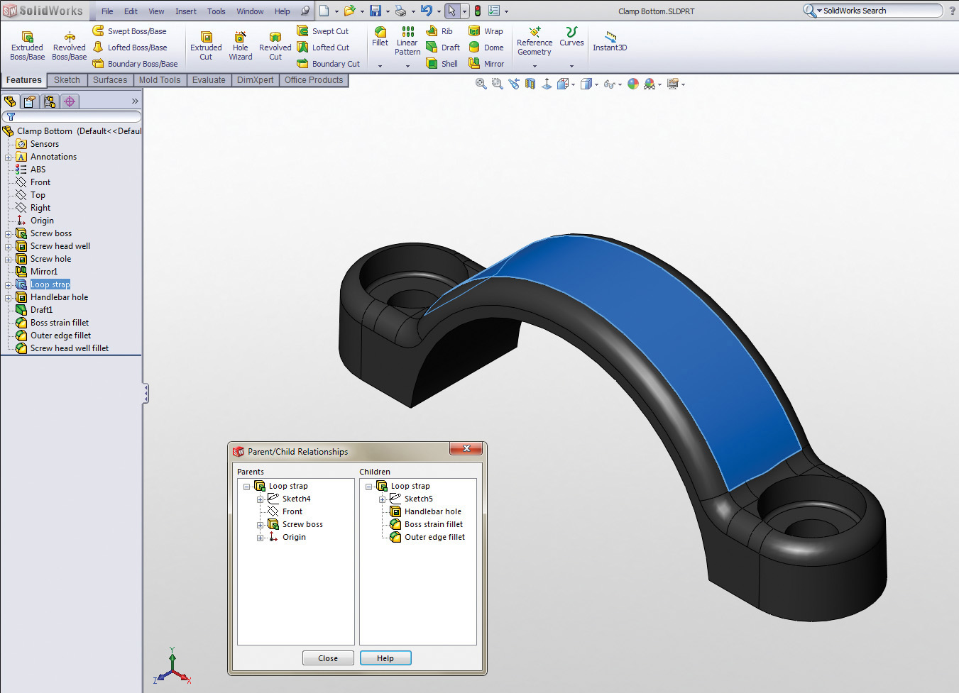
5.51 A tree diagram showing the dependencies between features can help you plan your parametric model. Notice how the list of parent and child features from this SolidWorks model shows the dependencies between features. (Courtesy of Salient Technologies, Inc. (www.salient-tech.com))
Many constraint-based modelers allow you to “play back” the model to see how it is being generated by the underlying parameters. The sequences shown in Figure 5.52 and Figure 5.53 illustrate how the features used to create the parts are ordered in relationships that reflect the design intent for the parts.
5.52 Base Feature. The base feature (Extrude 1) is the first feature created. (Courtesy of Mark Perkins.)
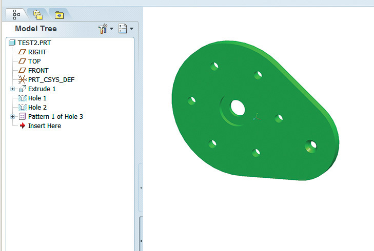
5.53 Child Features. Subsequent features are children of previous features. (Courtesy of Mark Perkins.)
Datum Planes and Surfaces
In engineering drawing, a datum is a theoretically exact point, axis, or plane. A datum provides a reference surface, axis, or point used for inspecting the manufactured part. Theoretically exact planes used in modeling are called datum planes. They are planes used as a reference for model geometry. You can also create datum axes and datum points in 3D models. Features can be constrained and dimensioned relative to these planes, axes, and points, even though they are not solid objects and add no mass to the model. Some modeling packages provide a set of three mutually perpendicular datum planes, located so that they pass through the origin of the coordinate system, as a default. You typically may also create additional datum planes at other orientations and locations.
Often, it is very useful to use a set of datum planes (three mutually perpendicular planes) as the base feature in your drawing. In fact, most software provides them as the default starting features. Figure 5.54 shows the shaft support part with a set of datum planes used as the base feature.
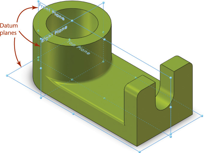
5.54 Datum Planes. The three mutually perpendicular planes in this drawing serve as the base feature for the model.
One of the benefits of starting with a set of datum planes is that they can provide a set of normal surfaces that you can use to orient sketch geometry. This is particularly helpful when there are no planar surfaces on the part that you can use to build subsequent features easily. With a cylinder as the base feature for the shaft support, for example, there is no flat surface to which the end of the base plate can be constrained to be parallel. The datum plane “Right Plane” in Figure 5.54 provides a reference to which the plate is parallel.
Whether or not you start with a set of datum planes as a base feature, consider the surfaces that will serve as datum surfaces on your part. Parts are inspected to see whether they were manufactured acceptably based on a similar set of three mutually perpendicular, theoretically exact planes. Measurements of the finished part are taken from surfaces coincident with one of the datum planes. As you define your features consider the dimensions that will determine whether the part will fit. How will the part be measured after manufacture? If there is a surface from which measurements will be taken, it can be advantageous to identify it as a datum surface in your part (see Figure 5.55).
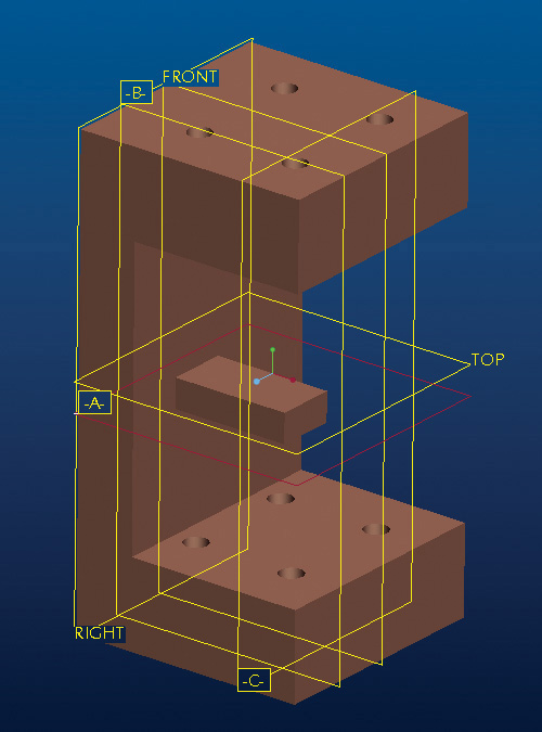
5.55 Datum Surface. Surface C on this fixture is a datum surface or reference location that will be used to inspect the location of a part feature. (Courtesy of Mark Perkins.)
Like the base point in a sketch, a datum plane serves as a reference from which the other features build. When you define a set of datum planes as the starting point for your model, you will be well on your way when deciding which datum surface to identify for use in inspecting the finished part.
Datum surfaces can also be helpful when defining tolerances for features. Defining your model using the dimensions that will be used to inspect the finished part will make it easier to determine the impact of variations from the stated dimension that occur during manufacture. (You will learn more about tolerances in Chapter 12.)
Datum planes also provide a common reference point for parts in an assembly. When parts share a set of datum planes, it is easier to align the part with other parts when you bring them together in an assembly model. If you do not use a set of datum planes as a base feature, you can locate new features from existing surfaces on the base feature.
Creating datum planes, lines, and points as base features can be used as a strategy called “skeleton modeling” (see Figures 5.56–5.58). Because the datums have no mass, they do not affect mass property calculations. They are easy to model and often do not change. For example, if you create a datum axis that is the centerline of the part, this is unlikely to change, whereas the shape of the part might. Even when some parts are not fully modeled or are represented only as a centerline, they can still be assembled using the datums as references.
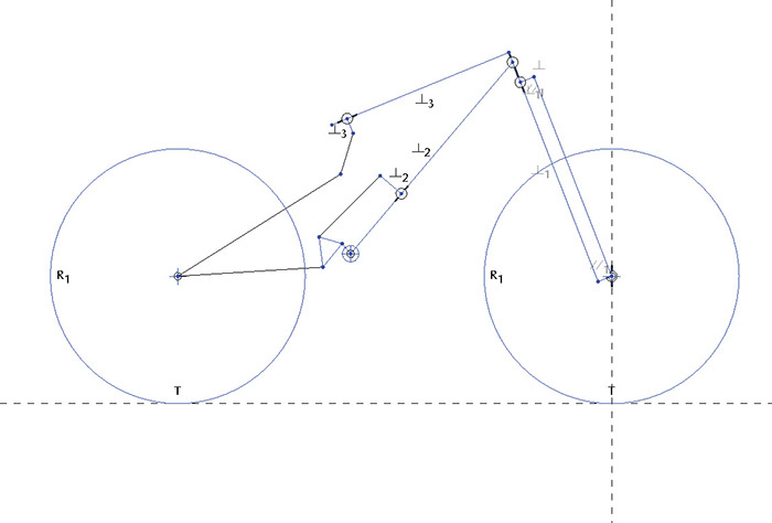
5.56 This constrained sketch acts as the skeleton for the bike assembly. It is made only of circles, lines, and points, which have no mass. (Courtesy of Santa Cruz Bicycles.)
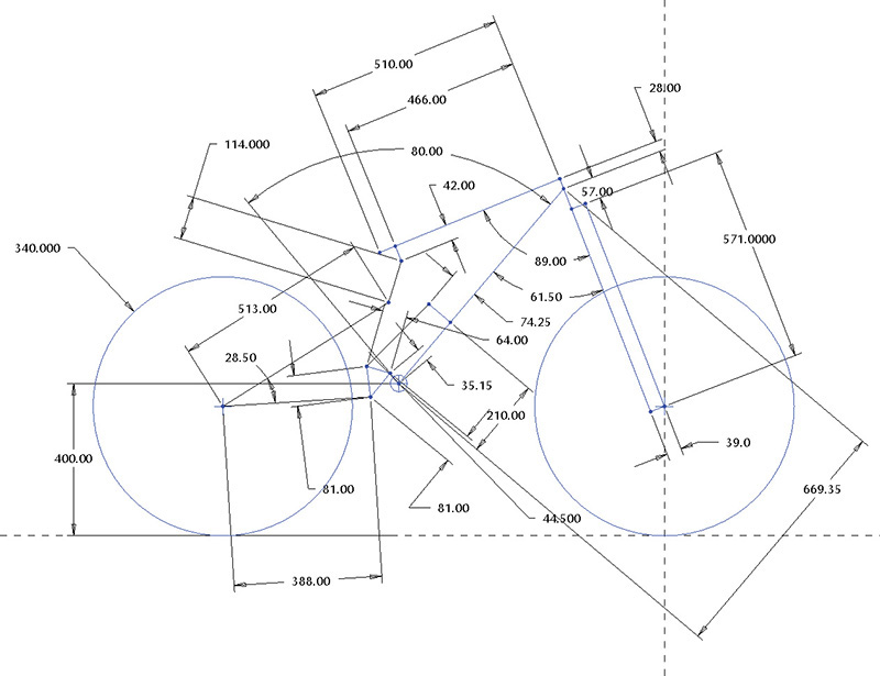
5.57 Dimensions are added to the constrained sketch defining the basic size relationships. These dimension values can easily be changed to try out different relationships. (Courtesy of Santa Cruz Bicycles.)

5.58 Parts can be assembled to, and even get their sizes directly from, the skeleton. This way parts can be viewed as assembled, even though all parts are not yet modeled. (Courtesy of Santa Cruz Bicycles.)
Datum planes and datum surfaces can be added and identified at any time, but considering them as you plan your model will help you use them more effectively in capturing design intent in your model.
5.9 Editing the Model
One of the biggest advantages of constraint-based modeling is that you can edit the features after they are created. If you have several parts open at a time in your software, you may have to identify which is the active part, then select the feature you want to edit. Once you select the feature you wish to edit, the dimensions for the feature are displayed in a way that lets you change their values. Alternatively, you can also return to the original sketch that you used to create the feature and modify the sketch. Figure 5.59 shows the shaft support drawing with a change being made to the overall length of the part.
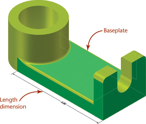
5.59 The length of the shaft support is changed by editing the dimension value and updating the model.
Depending on how the model was created, you may have more or less success in updating the model. For example, the baseplate that connects to the cylinder (indicated in the figure) can be created many different ways. Each way may have advantages or disadvantages for how the part will be updated.
Figure 5.60 shows three ways the baseplate could be generated:
a. Sketch the shape of the bottom surface on a sketch plane aligned with the bottom of the cylinder and extrude it upward.
b. Sketch the cross section on the midplane and extrude to both sides.
c. Sketch the rectangular end view on a plane offset parallel to the center datum plane and extrude the plate to meet the cylinder feature.

5.60 (a) Extruding upward; (b) extruding to both sides of a center plane; (c) extruding to the cylinder from an offset plane. All these methods could be used to generate the plate feature for the shaft support, but they update differently.
There are several other ways, too. Each of these methods works about the same when changing the length of the part. They vary if you decide to make the plate wider than the cylinder. Often, when a feature is extruded to an existing feature as in Figure 5.60c, the new feature cannot be updated so that it is wider than the surface to which it is extruded. The boundary, or end, of the feature is limited by the next surface. Where there is no portion of the surface at which the feature may end, it will continue to infinity and therefore be undefined.
Standard Features
Certain useful features are part of many engineering designs. Common features often have specific manufacturing processes developed to form them efficiently. For example, a counterbore is often used to create a recess for a bolt head or other fastener. Specific tools like the one shown in Figure 5.61 make it easy to form this feature.
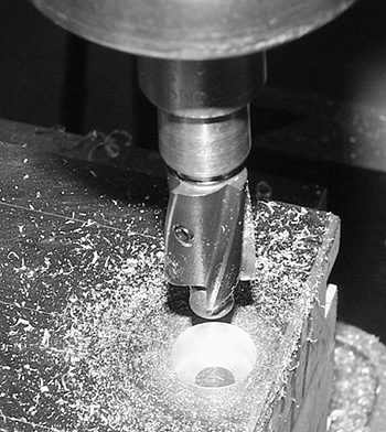
5.61 This counterbore tool on a milling machine makes a recess around the top of a hole. The center of the tool fits inside the hole to keep the counterbore concentric.
Many constraint-based modeling programs use the same terminology for these features as that used in manufacturing and design. Review the standard feature types on the next page.
Working with Built-in Features
Many standard features, such as counterbored and countersunk holes, fillets, lugs, slots, and others may be available in the constraint-based modeling program as built-in or placed features. These features can be placed with a dedicated command on part surfaces. Some features are solids, and others are negative solids that are subtracted from the model (for example, a cylindrical hole). The features have properties built into them that the modeling software will preserve, just as it preserves the geometric and size relationships you set.
Many constraint-based modelers provide a number of options for quickly placing holes, often through a “hole wizard” or other dialog box. Properties that can often be set for holes are listed in Table 5.4.
Through
|
The hole goes all the way through the part or feature. |
Blind
|
Material is removed to a specified depth |
Countersunk
|
A conical shape is also removed to allow for a countersunk tapered screw head. |
Counterbored
|
A cylindrical recess is formed, usually to receive a bolt head |
Spotface
|
A shallow recess like a counterbore is formed, used to provide a good bearing surface for a fastener. |

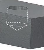
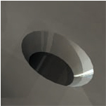


A Hole command may also allow you to choose the specialized constraints for locating holes, such as concentric, placed by edge, and on point, as illustrated in Figure 5.62.

5.62 Pro/ENGINEER’s Hole Wizard has many placement options as well as types of hole features available. (Courtesy of Mark Perkins.)
Many CAD systems have aids to creating features that are a part of many engineering designs (see Figure 5.63) that can make creating your model even easier.

Feature |
Example |
Fillet: A rounded interior blend between surfaces; used, for example, to strengthen adjoining surfaces or to allow a part to be removed from a mold |
|
Round: A rounded exterior blend between surfaces; used to make edges and corners easier to handle, improve strength of castings, and allow for removal from a mold |
|
Counterbore: A cylindrical recess around a hole, usually to receive a bolt head or nut |
|
Countersink: A cone-shaped recess around a hole, often used to receive a tapered screw head |
|
Spotface: A shallow recess like a counterbore, used to provide a good bearing surface for a fastener |
|
Boss: A short raised protrusion above the surface of a part, often used to provide |
|
Lug: A flat or rounded tab protruding from a surface, usually to provide a method for attachment |
|
Flange: A flattened collar or rim around |
|
Chamfer: An angled surface, used on a cylinder to make it easier to start into a hole, or a plate to make it easier to handle |
|
Neck: A small groove cut around the diameter of a cylinder, often where it changes diameter |
|
Keyway/Keyseat: A shaped depression cut along the axis of a cylinder or hub to receive a key, used to attach hubs, gears, and other parts to a cylinder so they will not turn on it |
|
Knurl: A pattern on a surface to provide for better gripping or more surface area for attachment, often used on knobs and tool handles |
|
Bushing: A hollow cylinder that is often used as a protective sleeve or guide, |
|

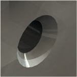

A fillet is a common built-in feature that rounds the edge formed by two surfaces. Typically, a fillet can be created by selecting the edges to be filleted (several can be selected at once) and specifying the radius of the fillet. A round is another type of standard feature created in the same way, usually using the same Fillet command. When the surfaces move or are lengthened, the fillet or round adjusts automatically. Figure 5.64 shows a typical fillet and a typical round with a uniform radius.
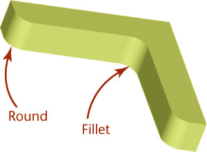
Sophisticated constraint-based modelers allow you to create uniform radius fillets and rounds, chained fillets and rounds that blend around a corner of a surface, constant-chord fillets and rounds, and variable-radius fillets and rounds (shown in Figure 5.65) using different methods. A constant-chord fillet is used in situations similar to Figure 5.65b, where a constant-radius fillet would result in thicker material on the uphill and downhill side of the blend. The constant-chord distance creates a fillet with a uniform amount of added material. More sophisticated blends between surfaces are also available in some software.

C0, C1, and C2 are terms used to describe the geometric continuity of surface blends (see Figure 5.66). (You may also see the letter G used as a designation for geometric continuity.)
• C0: Coincident surfaces meet but are not tangent. These are essentially intersecting surfaces, not ones that have a fillet.
• C1: Tangent surfaces meet and are tangent. This is the typical tangency produced by Fillet commands, and is suitable for most rounded edges.
• C2: Curvature continuous surfaces meet and are tangent, and where surfaces blend, they share a common center of curvature. Surface blends with this continuity do not have any abrupt change in radius. These blends are important for styling of surfaces such as automobile hoods and exterior plastic parts.
• C3: The next level above C2, except that the rate of change for the curvature is also continuous.
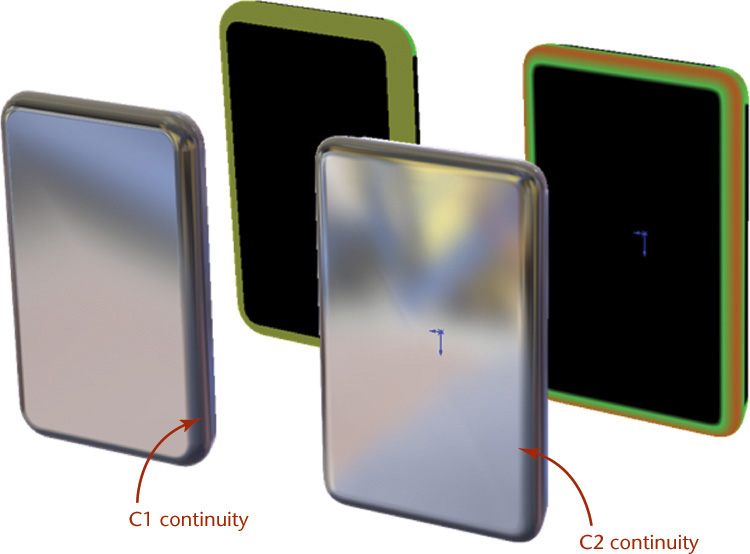
5.66 Surface Continuity. The iPhones above left were modeled with tangent surfaces: C1 continuity. The smoother blends of the models on the right use C2 continuity. (Images courtesy of ©2016 Dassault Systèmes SolidWorks Corporation.)
Complex Shapes
Complex shapes can often be made using special surface modeling commands that create surfaces that cannot easily be made with regular extrusion, revolution, sweeping, and blending. These surfaces can then be added to the model (see Figure 5.67). Once a surface has been added to the model and the edges completely matched (rather like being watertight), the object then can be “solidified” into a solid, which allows mass property calculations.

5.67 The open-surface model in (a) is patched and then “solidified” into a solid model (b). (Courtesy of Strategix Vision.)
Because the complex surface can slow down model regeneration, an approximation of the surface may be used as a placeholder until later in the refinement process.
5.10 Constraint-Based Modeling Modes
Most constraint-based modelers have three main modes that link together to provide a full range of functionality in creating and documenting your designs: part mode, which allows you to create individually manufactured parts of a single material; assembly mode, which allows you to link multiple parts together into assemblies (Figure 5.68) or subassemblies; and drawing mode, which allows you to create orthographic, section, and pictorial drawings to document the design.


Assemblies
Assembly capabilities in constraint-based modelers make concurrent engineering feasible. Companies can use the single design database as the hub of a collaborative environment for a cross-functional design team. Planning the critical relationships that capture the design intent of the assembly—just as would be done for each individual part—allows the constraint-based assembly to be used to coordinate efforts of several different individuals. The entire assembly and each part are stored in the design database for members of the design and manufacturing team to view, measure, or change (if authorized) while the parts are being designed.
The assembly provides a framework for the model. In the assembly, global parameters can be used to build intelligent assemblies. For example, if several parts assemble onto a shaft, the shaft diameter may be made a global parameter. The hole sizes on the parts that fit onto the shaft may be created by adding or subtracting a value from the global parameter for the shaft diameter. If the shaft diameter is changed, all the parts that fit with it may automatically be updated. Using global parameters can be an effective way to coordinate the design effort for a team. You will learn more about using assemblies to refine your design in Chapter 10.
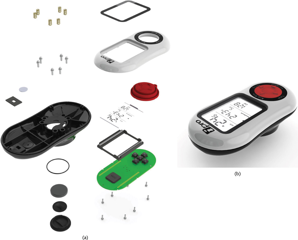
5.70 The parts that make up the iBike Pro cycling computer were modeled individually as solids, then combined into a single assembly model to represent the finished product. The exploded view in (a) shows the individual parts clearly; the assembled view in (b) shows how the parts will fit together. (Courtesy of iBike and Salient Technologies, Inc.)
Drawings from the Model
An advantage of solid modeling software is that drawings can be generated from the solid model. Creating drawings using constraint-based modeling software adds a significant dimension to this advantage: associativity.
Bidirectional Associativity
When a set of drawing views have been created from the model (Figure 5.71) and a change is made to the model, the drawing views will automatically be updated because they are associated with the actual model. Dimensions in most constraint-based modeling software control the sizes of the model features. The process of dimensioning a drawing can be automated because the software reports the dimension value for the entities in the CAD database.
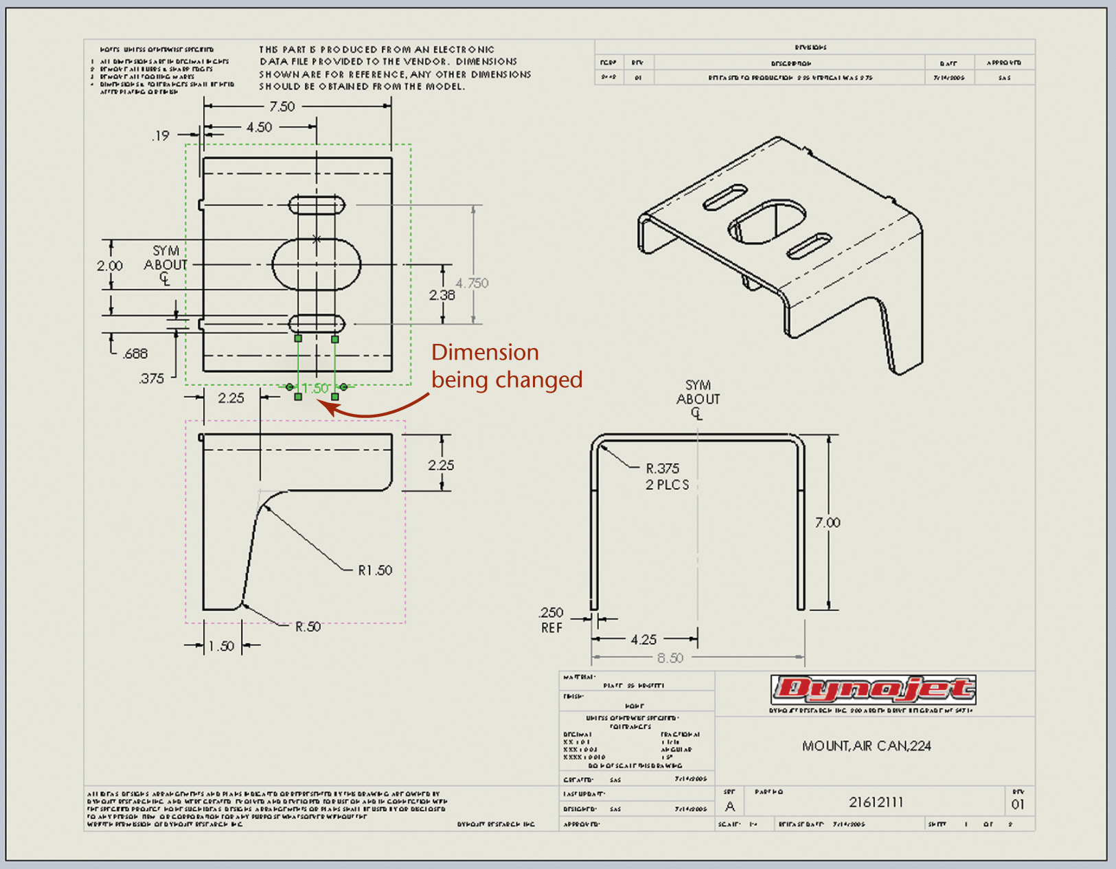
5.71 Associativity. The 1.50 dimension for the slot highlighted in green in the top view is changed in the drawing to the new size, 2.00. (Courtesy of Dynojet Research, Inc.)
If the size of a feature changes in the model, the value for the dimension in the drawing is automatically updated to show the correct values. When this is a oneway process—when changing the model causes the dimension value to be updated on the drawing—the dimensions are said to be associative. When this is a one-way process, changing the dimension value on the drawing has no effect on the model geometry. In fact, it may break the link between the dimension value and the model geometry.
Most constraint-based modelers are bidirectionally associative: changing a dimension in the drawing changes the model geometry, and vice versa (see Figures 5.71 and 5.72). Constraint-based modelers store and use the dimensions and constraints to generate the model. When dimensions are shown in a drawing, the values are the dimensions used to create the model. Whether these dimensions are changed in the part or on the drawing, the new values are stored in the database, and the model and all associated drawings are updated to reflect the new dimension values. Bidirectional associativity allows drawing changes to update the model, and model changes to update the drawings.
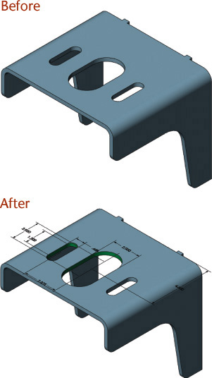
5.72 Bidirectional Associativity. The model for the mounting bracket is shown before (slot at 1.50) and after the dimension on the drawing was changed to 2.00. (Courtesy of Dynojet Research, Inc.)
Industry Case: Constraint-Based Modeling: Capturing Design Intent
When William Townsend was a Ph.D. student at MIT, he designed a four-axis robot arm that simulates the motion of the human arm. This human-scale dexterous arm works with the subsequently developed Barrett wrist and robot hand produced and manufactured by Townsend’s engineering firm, Barrett Technology. To prepare the design for larger-scale production, the original 2D drawings were converted to constraint-based solid models, which enhanced Barrett Technology’s ability to quickly make design changes and evaluate the results. By redesigning the robot arm, the company was able to make it the lightest one on the market and save 50% over previous manufacturing costs.
To benefit from constraint-based modeling, it was important to design the parts with the design goals in mind. “You need to keep your design intent in mind. Even though the software is a powerful tool, if you tie up a feature or overconstrain it, you are limiting the amount of flexibility you have in changing it easily later,” said Brandon Larocque, project manager at Barrett Technology.
The top plate of the BarrettHand is a good example of how Larocque approaches constraint-based design (see Figure 5.73). The part has a total of fourteen features and took about 30 minutes to model in SolidWorks. When a new part is created, SolidWorks provides a default set of three orthogonal planes that intersect at the origin. The user can add more planes, but SolidWorks allows any surface to be used as a sketch plane. Larocque estimates that 80% to 90% of the parts he models do not need additional sketch planes.

5.73 This rendered view of the BarrettHand clearly shows the top plate in relation to the rest of the hand.
The top plate of the hand began as half of a symmetrical sketch that was mirrored across the centerline (see Figure 5.74). The constraint-based relations in the mirrored half of the part were set up so they would be the same as those in the original half. To create the sketch, three radii were dimensioned to form the curved end of the plate: one in each corner and a larger one to form the curved end of the plate. The center of the largest radius is constrained to always lie on a horizontal construction line inserted into the base sketch. The other end-radii have tangency relationships where they meet the large radius and the straight lines that define the other edges of the plate. These tangency constraints were automatically created by SolidWorks when the radii were sketched in place. The three radii were constrained to be mutually tangent so the tool path generated by the model would be a single smooth curve through the three radii. The only other dimensions needed to define the part were those for the overall length of the part and the rectangular shape at the top of the part. All distances (dimensional constraints) were defined from the center of the part (which also coincided with the origin in SolidWorks). The sketch was then extruded to become the base feature for the part.
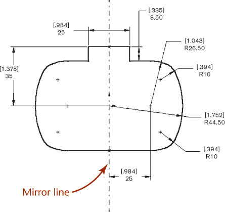
5.74 The sketch for the base feature is symmetrical about the centerline. Dimensions are in SI units with inch units in brackets.
When Larocque thinks about selecting a base feature, he chooses one that will support additional features and reflect the way the part may be modified and eventually built. “I think modeling in 3D is similar to the way a machinist shapes a part. The modeling operations give you some intuition about the steps required to make the part and how many different setups a part will require. If you can make all of your features from the same surface of a part, chances are the machinist will be able to make them from a single setup as well. If you can form a part with a single revolution, you can probably make the part on a lathe in a single setup. Each time you add a sketching plane that is not normal or parallel to the default planes, you can assume the part may require an additional setup in order to machine it. Reducing a part’s design from four setups to three can reduce the machining costs by 25%.” In the case of the top plate, all its features except the bevel and the counterbores were created from the same side of the part.
Because the plate is symmetrical, its center point also served as the design center of the part. The plate is designed to mate with two bearings set a specified distance apart. Dimensioning the part about a point at the intersection of the mirror line of the plate and a line through the center points of the two bearing bores means that any change in the distance between the bearings requires few changes to update the part.
The next step was to create the bevel around the outside of the base feature. Using the mirror plane (across which the first sketch was mirrored) as the sketching plane, Larocque sketched a triangular shape with a 30° angle (see Figure 5.75). This sketch was the profile for the bevel. A contour was sketched on the back surface of the plate to serve as the path for the triangular profile. After selecting both sketches, he used a sweeping operation to create the feature. SolidWorks prompted him to identify the profile (the triangle), the path (the contour sketch), and the sweep operation (a cut). The profile was dragged normal to the sweep path to cut the bevel on the plate. A machinist cutting this feature into actual metal would similarly use a 30° tapered mill to sweep out the same path defined in the model.

5.75 The triangular shape of the bevel is a sketch on the mirror plane that was swept along the contour.
The next feature hollowed out the part. Sketching on the surface of the part that lies on the original sketch plane, Larocque created half of the shape of the area to be removed, dimensioned it from the centerline, and mirrored it to create the complete outline. The sketch was then extruded to the appropriate depth to be cut from the base feature (see Figure 5.76).
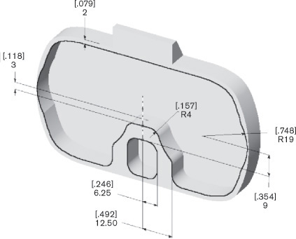
5.76 The sketch for hollowing out the plate included two distinct outlines that were extruded as a single feature.
The fourth feature was a semicircular cutout to provide clearance for a motor pinion (see Figure 5.77). This circle was sketched on the original sketching plane, its diameter was dimensioned, and its center point was constrained to the center of the part (which corresponds to the distance from the centers of the bearings). Using a constraint to position the feature on the part’s centerline guaranteed that the feature would stay centered even if the overall size of the part changed. To form the feature, Larocque specified a blind extrusion to a specified depth.
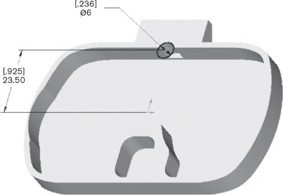
With the part hollowed out, the new interior surface was used as the sketch plane for the bosses that would be the bearing bores (see Figure 5.78). The bosses could have been formed on the initial sketching plane in the same operation that hollowed out the part, but their height would have been constrained by the depth of the part. If the depth were to change, the height of the bosses would, too. Using the new surface ensured that the relation of the bosses to the inside surface of the plate would remain constant, even if the depth of the surface changed.

To create the bosses, Larocque created symmetrical 20-millimeter circles with center points constrained to the horizontal centerline of the part. The circles were extruded, and two new concentric circles were sketched on the tops of the new features (see Figure 5.79). From the tops of the bosses, Larocque extruded cuts back toward the bottom. Because the boss is to serve as a bearing bore, the depth of the hole in the middle must correspond to the width of the bearing, not the height of the boss. Extruding the hole from the top of the boss means that the hole will remain at the same depth even if the boss becomes taller or shorter. The same process was repeated to make the two smaller bosses.
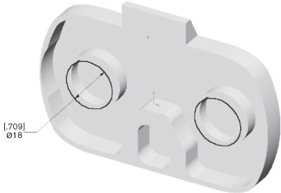
The next feature was a chamfer on the inside edges of the bearing bores. SolidWorks allowed Larocque to multi-select all the bosses at once, then insert a chamfer (see Figure 5.80). A chamfer is a built-in feature with its own dialog box for setting its angle and depth. The single operation created the four chamfers, all to the same specifications. They constitute a single feature that cannot be decoupled into individual chamfers. Independent control of each chamfer would require creating four separate features.

Another built-in feature, a fillet, was added next. Larocque selected the two corners where the rectangular protrusion intersected the body of the part and added both fillets with the same operation.
The H-shaped pocket at the top of the plate was sketched next as a symmetrical feature. This feature is an alignment pocket that should move with the bearing bores. Its location and radii were dimensioned from the center of the part (to coincide with the centers of the two 20-mm bosses), and its length constrained to the centerline of the part (see Figure 5.81). “Most of the features after the base feature are dimensioned from the bearing bores because they are the defining characteristic of the part. I set up a relationship between the bearing bores and the alignment pocket because the alignment pocket determines where the bearings will fall.”

The final features were the six holes and the counterbores to accommodate the fasteners to go into them. The first hole was given a diameter dimension, then the other holes were constrained to be the same size as the first (see Figure 5.82). All six were sketched on the sketch plane used for the bevel contour and extruded with the “through all” setting so they will always go all the way through the part, even if the part thickness changes. From the same side of the part, the counterbores were added to the holes as the final features. Larocque specified counterbores at the appropriate depth that are concentric with the hole (see Figure 5.83).
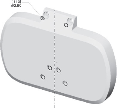
5.82 Only one of the holes displays a dimension here; the other five are constrained to the same diameter as the first.
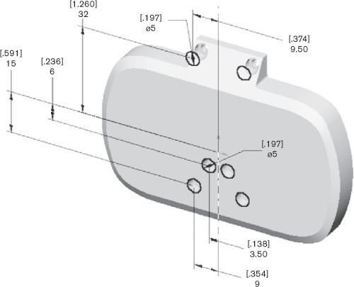
When asked about the degree to which he uses constraint-based relations, Larocque explained, “We like to keep the model somewhat segmented so we have more control over the updates, but we make sure to add relations where they make sense. For example, constraining symmetrical parts to a centerline as we did with the top plate of the hand can save enormous amounts of time when the part can update automatically. This aspect of the model was instrumental in our ability to make the BarrettHand lighter and less costly to manufacture.”
(Designs courtesy of Barrett Technology, LLC, Newton, MA.)
5.11 Choosing the Right Modeling Method
As you design, you will want to choose a modeling method that makes sense for your product, the stage in the design process, and the cost. Table 5.5 recaps the modeling methods according to the model qualities identified earlier in this chapter.
Table 5.5 Characteristics of Modeling Methods
Characteristic |
Paper Drawings |
2D Wireframe |
Physical Model |
Visual |
2D views require interpretation and may be less understandable to a nonengineer. |
2D views require interpretation and may be less understandable to a nonengineer. |
Similar to actual object. Can be seen from all angles. May be smaller scale, unrealistic material. |
Understandable |
May require experience interpreting multiview drawing technique to be understood. |
May require experience interpreting multiview drawing technique and descriptive geometry to be understood. |
Can interact in a way similar to real object to aid in understanding. May be different scale, material than real object. |
Flexible |
Changes require erasure; difficult to accommodate large changes without redrawing. |
Editing capabilities and layers make models more flexible than paper drawings. |
Can be modified to a degree, but substantial changes may require a new model. |
Cost-effective |
Low equipment costs, but man-hours may be greater than with other methods. Cost effective for visualization and documenting simple parts. May be necessary if electronic formats cannot be read. |
Useful for projects where the information gained from a 3D model is outweighed by the cost of capturing it, as in civil mapping and electrical circuit and distribution design. |
Varies with the information contained in the model (where more information is usually more expensive) and the cost of manufacturing errors that could be prevented by the model. |
Measurable |
Not suited to be measured from. |
Because objects are drawn full size, measurements may be taken from the model; knowledge of descriptive geometry required to derive information not shown in standard views. |
Depends on how closely the model matches the materials and processes to be used to create the actual product. |
Accurate |
Requires proper dimensions to reflect design accurately. |
Offers a high degree of accuracy when orthographic drawing techniques are understood. |
Depends on how closely the model matches the materials and processes to be used to create the actual product. |
Robust |
May require multiple views to fully define the shape of an object. |
More robust than paper drawings and can include links to large amounts of data; lacks information about volume found in 3D models. |
Can include as much information as the actual product. |
Application |
Effective for sketches and quickly conveying the design of simple parts for manufacturing. |
Useful for largely 2D information such as maps, layout drawings, and electrical circuits. |
Good for testing fit of parts, interaction with other products and people, and analyzing aspects that cannot be simulated. |
Key considerations are the time required to model the part and the purposes for which it will be used. A simpler method that provides all the needed information is more cost-effective than one that takes longer to model. However, time invested in a complete digital model of the product can pay for itself if it is used to generate visuals that help shape the design, reduce manufacturing difficulties, foster concurrent engineering—or promote the product later.
The accuracy of the modeling method is another key consideration. What types of analysis must be or could be completed with a model? What level of accuracy will be required to interface with CAM programs?
As you have seen, 3D modeling packages that are strong in surface modeling are needed to model the geometry of smoothly contoured features such as the ergonomic mouse shown earlier in the chapter. Piping systems and other structures of simple geometric shapes can sometimes be modeled very effectively using 3D wireframe modeling. Many inexpensive CAD packages support this type of modeling. However, a solid modeling package is required to create a model that can be used to check parts for fit and interference; calculate the weight of a final assembly from the many individual parts; generate a rendered view of the assembly that can be used in manufacturing, marketing, service and repair; and drive the computer-aided machinery to manufacture parts. The same assembly model created using constraint-based modeling methods would have the added advantage of being updated automatically when key dimensions change. It would also make it easy to create a family of similar parts.
Whether you choose the modeling package or learn to use the tools provided by your employer, you should be aware of the strengths and limitations of the software so you can use it most effectively.
Characteristic |
3D Wireframe |
Surface |
3D Solid |
Visual |
Can be viewed from any direction and used to create standard 2D views; lack of surfaces may make views ambiguous. |
Usually includes lighting and background options that can be used to create photo-realistic images of the model. |
Shaded and rendered views present a realistic view of the object; offers automated 2D view generation; with most equipment only 2D view is available on monitor; part must be rotated to picture clearly. |
Understandable |
Requires viewer to mentally add surfaces to see the 3D shape. |
Shaded views are easily understood by the viewer. |
Shaded views are easily understood by the viewer. |
Flexible |
Editable, but changing individual objects more time-consuming than in other methods. |
Each vertex is editable, but ease of changes depends on method used to create and store the surface. |
CSG or hybrid models offer the most flexibility; can edit at the level of the solid object instead of individual geometric entity. |
Cost-effective |
Requires less computing power, and software is generally lower priced; good for modeling geometrically simple shapes. |
Most cost-effective for modeling irregular surfaces that must be conveyed to manufacture with a high degree of accuracy; photo-realistic displays can offset modeling costs by adding value in marketing. |
Completeness of the solid model cost-effective when model can be used for multiple purposes, such as testing, presentation, and CAM. |
Measurable |
Full-size entities are measurable without auxiliary views; can only measure between wireframe entities, however. |
Can be used to calculate surface area. |
Can be used to measure not just size but also weight, mass, and other physical properties. |
Accurate |
Offers a high degree of accuracy for the entities represented. |
Depends on method used to store model data; smoothed surfaces generally more accurate than mesh surfaces. |
Depends on method used to store model data; high degree of accuracy possible. |
Robust |
Model stores only vertices and edges; lacks surface or volume information; may be ambiguous as to voids or holes. |
Fully defines the surfaces of a part; lacks volume information. |
Includes volume as well as surfaces and vertices; can eliminate need for physical model. |
Application |
Good for applications where relationships in 3D space must be modeled, simple geometric shapes are sufficient for the objects to be modeled, and realistic views are not required. |
Good for designs that include irregular or free-flowing surfaces and for those where the appearance of the product is a critical design criterion. |
Good for applications where fit between parts and other engineering properties need to be evaluated before manufacture. |
Industry Case: Choosing the Right Method: Surface Modeling
The Stryker SmartPump tourniquet system continuously monitors and controls tourniquet pressure during surgeries (Figure 5.84). When Kent Swendseid, Design Director at Strategix Vision, designed the enclosure for the product, he used surface modeling techniques to obtain the smooth curves envisioned for the case and built-in handle.
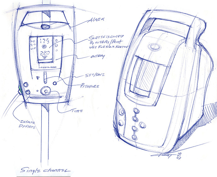
Before these outside surfaces were modeled, the internal components and user interface were worked out to determine the shape and volume required. Concept sketches were done (including rough models in 3D) to show various options for the enclosure. Once a concept was chosen and the internal configuration was known, surface modeling started in earnest.
Swendseid used a modeling approach that works well for complex molded assemblies: a “base part” controlling the overall shape and dimensions of the assembly is modeled first, then the component parts are derived from the base part. This way, if something in the design has to change, only the base part has to be modified to alter the exterior. The derived parts are updated accordingly. This approach also allows various parts to be modeled in parallel by a team rather than a single designer.
The case concept was a clamshell of two large molded parts with a molded-in handle. The first step was to identify key features, such as where and how the two molded parts would come together, and where mounting positions for things like the display would be. These were represented as planes in the model. Shapes and contours important to the shape were also created early in the modeling and are visible in the feature tree for the part (see Figure 5.85). These changed as modeling progressed, but because the model was built around them, it was simple to update.

5.85 The feature tree for the base part consists of planes and reference lines that other features are derived from and constrained to.
The front face was modeled as a loft—a surface that morphs from one curve to another. The curvature was controlled by either guide curves or tangency constraints at the ends (Figure 5.86). Early surfaces are almost always modeled larger than the face that will end up on the part to simplify manipulation of the curvature—and to avoid unwanted edge effects.
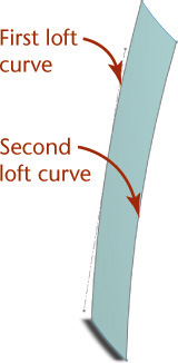
The next surfaces added do not show up in the final model directly. These “helper surfaces” can be used to control the angle where two surfaces meet (Figure 5.87). To ensure that the surfaces of the mold will let go of the part when it is ejected, the surface has to have what’s known as “draft”—the surface has to sit at an angle to the direction the mold opens. Creating a simple helper surface at the parting plane provides a draft constraint to which to tie a more complex surface: if the surface is tangent to a surface with enough draft, it will have enough draft too. Helper surfaces are trimmed off, deleted, or hidden when no longer needed.
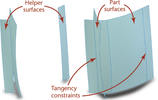
Additional faces were built using swept, extruded, and revolved surfaces to define half of the symmetrical shape of the case. Using the symmetry does more than save work; it also guarantees that the model will actually be symmetrical. For a surface model, it also ensures that there will be no visible artifact where the two parts join. This avoids distracting highlights and waviness in the finished part.
In Figure 5.88, you can see that the part surfaces were modeled to extend beyond their intersections with other surfaces, thus allowing the software to calculate the intersections mathematically to create the edges between surfaces. It also means that simpler profiles can be used to loft or sweep the surfaces. The mathematics of surface modeling favors using the fewest possible constraints, because more constraints require higher-order polynomials to describe the surface. If the spline defining the intersection were used to generate the surface, tiny perturbations in the driving geometry could result in ripples or other undesired effects in the surface.
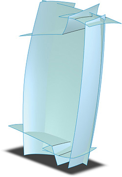
Trimming forms the boundary between surfaces. This operation can be used to create hard edges, but in this case the shape required a rounded edge. This requirement could be met with a fillet, but the designer wanted to avoid the sudden change of curvature where the fillet meets the two surfaces it joins. This is a common desire in product modeling, especially with glossy surfaces that reveal the change of curvature as an unwanted highlight instead of a smooth 3D curve. The designer also wanted to “bulge” the rounded edge toward the top and bottom, which would have required a variable-radius fillet—at the time, an unreliable feature.
To create the rounded edge, the front and side surfaces were trimmed to helper surfaces that described the boundary (Figure 5.89, left) and the gap was filled with another loft, which allowed the result to be curvature-continuous. Note that the top and bottom of the two surfaces in Figure 5.89 (middle) still extend beyond where they will eventually end, again to minimize the number of constraints on the fill surface.
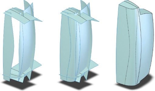
The order in which operations are done affects modeling efficiency. Sometimes it makes sense to leave trimming and joining surfaces to the very end, and sometimes it makes sense to join them earlier to simplify selecting them for other operations.
For example, the device mounts by fitting around a vertical pole behind it, so the case needed an indentation to clear the pole. Because the pole clearance surface crossed several others, modeling this feature was delayed until the rest of the device had taken shape (see Figure 5.90).
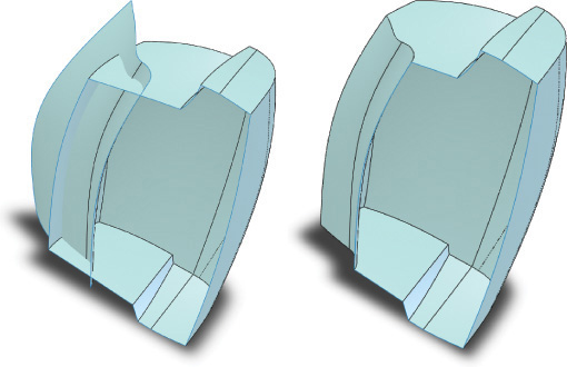
When it came time to add the handle opening, ergonomic concerns and balance issues made it difficult to use the main parting plane of the base part. The handle does not symmetrically straddle the main parting plane, so where the two halves of the clamshell would come together would be very close to the front edge of the handle. Because this would make it uncomfortable to hold the unit, the boundary of the part inside the handle was shifted rearward toward the middle of the handle. The handle opening was given its own parting plane.
The front opening for the handle area was then modeled in one feature (Figure 5.91). The face at the front of the handle was deleted to open up the edges, and those edges were captured as a compound curved profile. The inner opening was sketched on the handle parting line plane, and a surface was lofted between the two curves. The rear opening was handled similarly, as were the transition surfaces from the front of the case to the opening for the screen.

Once the surface half is complete, it can be “closed.” This turns the surface model into a solid model. Actually, a solid model is a surface model, just an “airtight” one with no open edges.
With a symmetrical model, the easiest way to close the model is to knit (join at the edges) a planar surface at the symmetry plane to the open edges of the model (see Figure 5.92, middle). Some modelers then automatically assume the model is a solid, but some have to be told to check for edge gaps and missing faces before changing the status of the body.
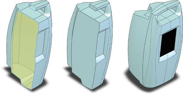
Once the model is solidified, it can be mirrored, non-symmetrical features can be added, and the surface can be used in later design stages (see Figure 5.93). In some cases, it can make sense to mirror the surfaces themselves, but that can increase the likelihood of small mathematical errors owing to the more complex nature of the boundary.
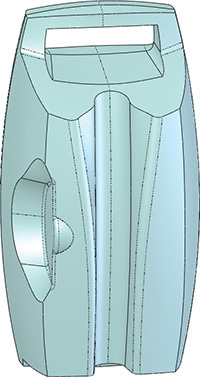
Building a model from a base part allows detail work to be started even before modeling of the base part is complete. As long as the surface can be closed and a solid formed, that solid can be shelled and split up into components. As additional features are added they are derived from the base part geometry so they will be updated if the base part changes. Figure 5.94 shows this kind of detailing in the rear half of the assembly.
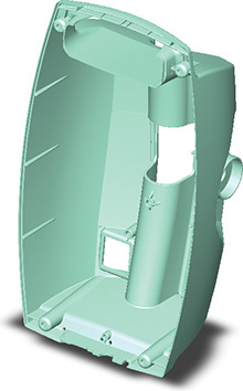
(All figures courtesy of Strategix Vision team members Kent Swendseid, Marty Albini, and Aki Hirota.)
5.95 Solid modeling was Albert Brown’s choice for refining the design of the parts shown in this sketch. The coaxial cable was formed by revolution; the cast arm was extruded and the holes formed with a Boolean operation. The wire clamp was created by sweeping its cross-sectional shape along a curved path. The resulting solid model allowed Brown to check the fit of the wire clamp. (Courtesy of Albert W. Brown, Jr.)
5.96 Concept sketches for this surgical device reveal several options for the enclosure, which was modeled using surface techniques. (Courtesy of Strategix Vision.)
Constraint-Based or Parametric Modeling
Triangulated Irregular Networks
Chapter Summary
Now that you have completed this chapter you should be able to list the qualities that models have that make them useful in the design process. You should be able to describe four CAD modeling methods that you might use to refine your design ideas. Not all modeling methods capture the same amount of information about the parts or device. You should be able to select the best modeling method to use for a particular design problem. The exercises allow you to test your understanding of the modeling process, ask you to apply a particular CAD modeling process to a design problem, provide practice with your modeling package, and ask you to decide which modeler you would choose to design a particular object.
You should be able to list advantages of constraint-based modeling over solid modeling. You should be able to correctly use the term parent-child relationships as applied to part features. Associativity between drawing views and the 3D model is an key characteristic of sophisticated constraint-based modeling programs. Selecting the base feature of the model is important, as it is the first parent feature. The exercises ask you to demonstrate your understanding of parent-child relationships and base features by capturing design intent in a number of part models. They also provide additional practice with your constraint-based modeling package.
Review Questions
1. You are a member of a team designing an automatic door-opening device so wheelchair users can enter and exit buildings on campus. Which of the modeling methods available to your design team are appropriate in each of the following situations:
a. Preliminary design review with your immediate engineering (technical) supervisor
b. Discussions of installation details with the campus architectural staff
c. Meeting with a group of nontechnical advocates for accessibility by persons with disabilities
d. Meeting with machine shop technicians who will fabricate your prototype
2. Which modeling method contains the most information about a design? Identify a situation in which this would not be the best model to use.
3. Recent developments in Global Positioning System (GPS) technology have resulted in small, relatively inexpensive, handheld GPS receivers (Figure 5.97).

a. A need exists for a mount to attach the system to mountain bikes in such a way that the display is visible while the rider is mounted. It is not desirable to modify the GPS to provide attachment. Consideration should be given to protecting the electronics and display from damage during rugged use while providing a clear sky view for the built-in antenna. What types of CAD models could be used to develop this mounting attachment?
b. At what stage of the process would each type of model be appropriate?
4. For the following situations, choose a modeling method and explain why you would use it.
a. Designing a prosthetic limb
b. Routing a piping system for a building
c. Designing a one-of-a-kind machined part
d. Verifying clearances for an electrical substation located near an airfield
e. Mapping an oil reservoir
5. Not all machines have moving parts. A wedge is an example of a simple machine. Use each of the modeling methods discussed in the chapter to model a wedge. Use the same size wedge for each model.
6. Constraint-based, or feature-based, modeling uses defined relationships between model elements to control various features. What two basic types of constraints are used to control features?
7. Why are the linear, angular, or other physical dimensions of a constraint-based model feature given a name? Give an example where this practice might be useful.
8. An acronym sometimes used to describe the process of preparing for the creation of a constraint-based model is TAP, representing the steps Think, Analyze, and Plan. Consider what it means to think, analyze, and plan a constraint-based model. Why are these steps especially important prior to beginning the constraint-based model?
9. What is meant by parent-child relationship in constraint-based modeling?
10. Define bidirectional associativity with respect to a constraint-based modeling program’s drawing mode. How does this program feature enhance ease of use of the program?
11. You are considering modifying a model by changing dimensions in a drawing view. What problems might you encounter when using a constraint-based modeler without bidirectional associativity? What problems might you anticipate when using a constraint-based modeler with bidirectional associativity in this task?
Chapter Exercises
Exercise 5.1 The toy building blocks in the photos are assembled by inserting the posts on top of one block into the space around the central circular extrusion on the bottom of another block The parts are made of molded plastic. Consider the design intent for these blocks. What dimensions are critical so these blocks will fit together in different arrangements? Create a model of a six-post block (2 × 3). Update your model to contain eight posts (2 × 4), as in the block at right.
Exercise 5.2 For each part shown, list the modeling method you would choose to create it if you were creating the original product definition for mass-producing these items. Give the reasons for your choices.