Chapter 9 Reaction Mechanisms, Pathways, Bioreactions, and Bioreactors

Search in book...
Toggle Font Controls
Create new playlist

Name your new playlist

Playlist description (optional)
Sign In

Email address

Password

Forgot Password?

or

Continue with Facebook

Continue with Google
Sign Up

Full Name

Email address

Confirm Email Address

Password

or

Continue with Facebook

Continue with Google

9. Reaction Mechanisms, Pathways, Bioreactions, and Bioreactors

The next best thing to knowing something is knowing where to find it.

—Samuel Johnson (1709–1784)

Overview. The topics of this chapter include the pseudo-steady state hypothesis (PSSH), enzyme mechanisms and reaction kinetics, and the growth of microorganisms.

We start with Section 9.1 where we discuss PSSH and the formation of active intermediate species, which disappear as fast as they are formed. Next we show how we apply the PSSH to active intermediate species to develop rate laws for chemical reactions that do not follow elementary rate laws.

To develop rate laws for nonelementary reactions we

• choose an active intermediate and a reaction mechanism,

• write the elementary rate law for each reaction in the mechanism,

• write the net rates of reaction for each species, and

• invoke the PSSH for the active intermediates in order to arrive at a rate law that is consistent with experimental observation.

In Section 9.2 we apply the PSSH to biochemical reactions, with a focus on enzymatic reaction mechanisms and kinetics. Here, we study

• Michaelis–Menten kinetics,

• Lineweaver–Burk plot and other plots to analyze data, and types of enzyme inhibition and the corresponding rate laws.

In Section 9.3 we study the growth of microorganisms. Microorganism growth logically follows the discussion of enzyme kinetics because of the similarity of the Michaelis–Menten rate law and the Monod growth law. Here we study

• balances on the cell mass and the substrate,

• kinetics of cell growth,

• yield coefficients relating to cell growth on substrate consumption, and

• bioreactors.

We will use these principles to model both batch reactors and CSTRs, which are called chemostats. We should note that microorganism growth is becoming of increasing interest because of the use of algae as a biofuel.

9.1 Active Intermediates and Nonelementary Rate Laws

In Chapter 3 a number of simple power-law models, e.g.,

- r_{A} = k C_{A}^{n}

$- r_{A} = k C_{A}^{n}$

were presented, where n was an integer of 0, 1, or 2 corresponding to a zero-, first-, or second-order reaction. However, for a large number of reactions, the orders are noninteger, such as the decomposition of acetaldehyde at 500˚C

C H_{3} C H O \to C H_{4} + C O

$C H_{3} C H O \to C H_{4} + C O$

where the rate law developed in problem P9-5_B(b) is

- r_{C H_{3} C H O} = k C_{C H_{3} C H O}^{3 / 2}

$- r_{C H_{3} C H O} = k C_{C H_{3} C H O}^{3 / 2}$

The rate law could also have concentration terms in both the numerator and denominator such as the formation of HBr from hydrogen and bromine

H_{2} + B r_{2} \to 2 H B r

$H_{2} + B r_{2} \to 2 H B r$

where the rate law developed in problem P9-5_B(c) is

r_{H B r} = \frac{k_{1} C_{H_{2}} C_{B r_{2}}^{3 / 2}}{C_{H B r} + k_{2} C_{B r_{2}}}

$r_{H B r} = \frac{k_{1} C_{H_{2}} C_{B r_{2}}^{3 / 2}}{C_{H B r} + k_{2} C_{B r_{2}}}$

Rate laws of this form usually involve a number of elementary reactions and at least one active intermediate. An active intermediate is a high-energy molecule that reacts virtually as fast as it is formed. As a result, it is present in very small concentrations. Active intermediates (e.g., A*) can be formed by collision or interaction with other molecules.

A + M → A* + M

Properties of an active intermediate A*

Here, the activation occurs when translational kinetic energy is transferred into internal energy, i.e., vibrational and rotational energy.¹ An unstable molecule (i.e., active intermediate) is not formed solely as a consequence of the molecule moving at a high velocity (high translational kinetic energy). The energy must be absorbed into the chemical bonds, where high-amplitude oscillations will lead to bond ruptures, molecular rearrangement, and decomposition. In the absence of photochemical effects or similar phenomena, the transfer of translational energy to vibrational energy to produce an active intermediate can occur only as a consequence of molecular collision or interaction. Collision theory is discussed in the Professional Reference Shelf in Chapter 3 (http://www.umich.edu/~elements/5e/03chap/prof.html) on the CRE Web site. Other types of active intermediates that can be formed are free radicals (one or more unpaired electrons; e.g., CH₃•), ionic intermediates (e.g., carbonium ion), and enzyme-substrate complexes, to mention a few (http://www.umich.edu/~elements/5e/09chap/prof.html).

¹ W. J. Moore, Physical Chemistry (Reading, MA: Longman Publishing Group, 1998).

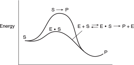
The idea of an active intermediate was first postulated in 1922 by F. A. Lindemann, who used it to explain changes in the reaction order with changes in reactant concentrations.² Because the active intermediates were so short-lived and present in such low concentrations, their existence was not really definitively confirmed until the work of Ahmed Zewail, who received the Nobel Prize in Chemistry in 1999 for femtosecond spectroscopy.³ His work on cyclobutane showed that the reaction to form two ethylene molecules did not proceed directly, as shown in Figure 9-1(a), but formed the active intermediate shown in the small trough at the top of the energy barrier on the reaction-coordinate diagram in Figure 9-1(b). As discussed in Chapter 3, an estimation of the barrier height, E, can be obtained using computational software packages such as Spartan, Cerius², or Gaussian as discussed in the Molecular Modeling Web Module in Chapter 3 on the CRE Web site, www.umich.edu/~elements/5e/index.html.

Two reaction-coordinate graphs are shown.

In two reaction-coordinate graphs, the horizontal axis represents Reaction Coordinate and the vertical axis represents Energy. In graph (a) at left, a bell-shaped curve is drawn with cyclobutane (four CH subscript 2 molecules single-bonded with each other in the form of a square) labeled at left bottom of the curve and two ethylene molecules (a pair of CH subscript 2 double-bonded with CH subscript 2) at right bottom indicating that cyclobutane forms two molecules of ethylene. In graph (b) at right, a bell-shaped curve is drawn with a small trough at the top of the curve. The vertical distance from a horizontal line, from the bottom of the curve to the bottom of the small trough, at the top of the curve, is indicated as E. Cyclobutane (four carbon atoms single-bonded in the form of a square) at left bottom of the curve forms an active intermediate above the small trough at the top of the curve. The intermediate is in the form of four carbon atoms placed in the form of a square single-bonded with one another except the top two carbon atoms which are not bonded. Two ethylene molecules (a pair of CH subscript 2 double-bonded with CH subscript 2) are at the right bottom of the curve. The curve indicates that cyclobutane in a reversible reaction forms an intermediate which in turn forms two molecules of ethylene.

Figure 9-1 Reaction coordinate. Ivars Peterson, “Chemistry Nobel spotlights fast reactions,” Science News, 156, 247 (1999).

² F. A. Lindemann, Trans. Faraday. Soc., 17, 598 (1922).

³ J. Peterson, Science News, 156, 247 (1999).

Schematic shows a spider web connected to a mouse through a wire.

9.1.1 Pseudo-Steady-State Hypothesis (PSSH)

In the theory of active intermediates, decomposition of the intermediate does not occur instantaneously after internal activation of the molecule; rather, there is a time lag, although infinitesimally small, during which the species remains activated. Zewail’s work was the first definitive proof of a gas-phase active intermediate that exists for an infinitesimally short time. Because a reactive intermediate reacts virtually as fast as it is formed, the net rate of formation of an active intermediate (e.g., A*) is zero, i.e.,

\begin{matrix} r_{A *} \equiv 0 & (9-1) \end{matrix}

$\begin{matrix} r_{A *} \equiv 0 & (9-1) \end{matrix}$

This condition is also referred to as the Pseudo-Steady-State Hypothesis (PSSH). If the active intermediate appears in n reactions, then

PSSH

$\begin{matrix} r_{A*} = \sum_{i=1}^{n} r_{iA*} = 0 & (9 - 2) \end{matrix}$ $\begin{matrix} r_{A*} = \sum_{i=1}^{n} r_{iA*} = 0 & (9 - 2) \end{matrix}$

To illustrate how rate laws of this type are formed, we shall first consider the gas-phase decomposition of azomethane, AZO, to give ethane and nitrogen

(C H_{3})_{2} N_{2} \to C {}_{2}H_{6} + N_{2}

$(C H_{3})_{2} N_{2} \to C {}_{2}H_{6} + N_{2}$

Experimental observations show that the rate of formation of ethane is first order with respect to AZO at pressures greater than 1 atm (relatively high concentrations)⁴

⁴ H. C. Ramsperger, J. Am. Chem. Soc., 49, 912.

r_{C_{2} H_{6}} α C_{A Z O}

$r_{C_{2} H_{6}} α C_{A Z O}$

and second order at pressures below 50 mmHg (low concentrations):

r_{C_{2} H_{6}} α C_{AZO}^{2}

$r_{C_{2} H_{6}} α C_{AZO}^{2}$

Why the reaction order changes

We could combine these two observations to postulate a rate law of the form

- r_{A Z O} = \frac{k_{1} C_{A Z O}^{2}}{1 + k_{2} C_{A Z O}}

$- r_{A Z O} = \frac{k_{1} C_{A Z O}^{2}}{1 + k_{2} C_{A Z O}}$

To find a mechanism that is consistent with the experimental observations, we use the steps shown in Table 9-1.

TABLE 9-1 STEPS TO DEDUCE A RATE LAW

1. Propose an active intermediate(s).

2. Propose a mechanism, utilizing the rate law obtained from experimental data, if possible.

3. Model each reaction in the mechanism sequence as an elementary reaction.

4. After writing rate laws for the rate of formation of desired product, write the rate laws for each of the active intermediates.

5. Write the net rate of formation for the active intermediate and use the PSSH.

6. Eliminate the concentrations of the intermediate species in the rate laws by solving the simultaneous equations developed in Steps 4 and 5.

7. If the derived rate law does not agree with experimental observation, assume a new mechanism and/or intermediates and go to Step 3. A strong background in organic and inorganic chemistry is helpful in predicting the activated intermediates for the reaction under consideration.

We will now follow the steps in Table 9-1 to develop the rate law for azomethane (AZO) decomposition, –r_AZO.

Step 1. Propose an active intermediate. We will choose as an active intermediate an azomethane molecule that has been excited through molecular collisions, to form AZO*, i.e., [(CH₃)₂N₂]*.

Step 2. Propose a mechanism.

Mechanism ${\begin{cases} R e a ctio n 1 : & (C H_{3})_{2} N_{2} + (C H_{3})_{2} N_{2} \overset{k_{1AZO*}}{\to} (C H_{3})_{2} N_{2} + [(C H_{3})_{2} N_{2}]^{*} \\ R e a c t i o n 2 : & [(C H_{3})_{2} N_{2}]^{*} + (C H_{3})_{2} N_{2} \overset{k_{2AZO*}}{\to} (C H_{3})_{2} N_{2} + (C H_{3})_{2} N_{2} \\ R e a c t i o n 3 : & [(C H_{3})_{2} N_{2}]^{*} \overset{k_{3AZO*}}{\to} C_{2} H_{6} + N_{2} \end{cases}$ ${\begin{cases} R e a ctio n 1 : & (C H_{3})_{2} N_{2} + (C H_{3})_{2} N_{2} \overset{k_{1AZO*}}{\to} (C H_{3})_{2} N_{2} + [(C H_{3})_{2} N_{2}]^{*} \\ R e a c t i o n 2 : & [(C H_{3})_{2} N_{2}]^{*} + (C H_{3})_{2} N_{2} \overset{k_{2AZO*}}{\to} (C H_{3})_{2} N_{2} + (C H_{3})_{2} N_{2} \\ R e a c t i o n 3 : & [(C H_{3})_{2} N_{2}]^{*} \overset{k_{3AZO*}}{\to} C_{2} H_{6} + N_{2} \end{cases}$

In reaction 1, two AZO molecules collide and the kinetic energy of one AZO molecule is transferred to the internal rotational and vibrational energies of the other AZO molecule, and it becomes activated and highly reactive (i.e., AZO*). In reaction 2, the activated molecule (AZO*) is deactivated through collision with another AZO by transferring its internal energy to increase the kinetic energy of the molecules with which AZO* collides. In reaction 3, this highly activated AZO* molecule, which is wildly vibrating, spontaneously decomposes into ethane and nitrogen.

Step 3. Write rate laws.

Because each of the reaction steps is elementary, the corresponding rate laws for the active intermediate AZO* in reactions (1), (2), and (3) are

Note: The specific reaction rates, k, are all defined wrt the active intermediate AZO*.

(1) $\begin{matrix} r_{1 AZO*} = k_{1 AZO*} C_{A Z O}^{2} & (9-3) \end{matrix}$ $\begin{matrix} r_{1 AZO*} = k_{1 AZO*} C_{A Z O}^{2} & (9-3) \end{matrix}$

(2) $\begin{matrix} r_{2 AZO*} = - k_{2 AZO*} C_{2 AZO*} C_{A Z O} & (9-4) \end{matrix}$ $\begin{matrix} r_{2 AZO*} = - k_{2 AZO*} C_{2 AZO*} C_{A Z O} & (9-4) \end{matrix}$

(3) $\begin{matrix} r_{3AZO*} = - k_{3AZO*} C_{AZO*} & (9-5) \end{matrix}$ $\begin{matrix} r_{3AZO*} = - k_{3AZO*} C_{AZO*} & (9-5) \end{matrix}$

$(L e t k_{1} = k_{1 A Z O *}, k_{2} = k_{2 A Z O *}, a n d k_{3} = k_{3 A Z O*})$ $(L e t k_{1} = k_{1 A Z O *}, k_{2} = k_{2 A Z O *}, a n d k_{3} = k_{3 A Z O*})$

The rate laws shown in Equations (9-3) through (9-5) are pretty much useless in the design of any reaction system because the concentration of the active intermediate AZO* is not readily measurable. Consequently, we will use the Pseudo-Steady-State-Hypothesis (PSSH) to obtain a rate law in terms of measurable concentrations.

Step 4. Write rate of formation of product.

We first write the rate of formation of product

$\begin{matrix} r_{C_{2} H_{6}} = k_{3} C_{{AZO}^{*}} & (9 - 6) \end{matrix}$ $\begin{matrix} r_{C_{2} H_{6}} = k_{3} C_{{AZO}^{*}} & (9 - 6) \end{matrix}$

Step 5. Write net rate of formation of the active intermediate and use the PSSH.

To find the concentration of the active intermediate AZO*, we set the net rate of formation of AZO* equal to zero,⁵ r_AZO* ≡ 0.

⁵ For further elaboration on this section, see R. Aris, Am. Sci., 58, 419 (1970).

\begin{matrix} r_{AZO*} = & r_{1 AZO*} + r_{2 AZO*} + r_{3 AZO*} = 0 \\ = & \begin{matrix} k_{1} C_{A Z O}^{2} - k_{2} C_{AZO*} C_{A Z O} - k_{3} C_{AZO*} = 0 \end{matrix} & (9-7) \end{matrix}

$\begin{matrix} r_{AZO*} = & r_{1 AZO*} + r_{2 AZO*} + r_{3 AZO*} = 0 \\ = & \begin{matrix} k_{1} C_{A Z O}^{2} - k_{2} C_{AZO*} C_{A Z O} - k_{3} C_{AZO*} = 0 \end{matrix} & (9-7) \end{matrix}$

Solving for C_AZO*

\begin{matrix} C_{AZO*} = \frac{k_{1} C_{A Z O}^{2}}{k_{2} C_{A Z O} + k_{3}} & (9-8) \end{matrix}

$\begin{matrix} C_{AZO*} = \frac{k_{1} C_{A Z O}^{2}}{k_{2} C_{A Z O} + k_{3}} & (9-8) \end{matrix}$

Step 6. Eliminate the concentration of the active intermediate species in the rate laws by solving the simultaneous equations developed in Steps 4 and 5. Substituting Equation (9-8) into Equation (9-6)

$\begin{matrix} r_{C_{2} H_{6}} = \frac{k_{1} k_{3} C_{AZO}^{2}}{k_{2} C_{AZO} + k_{3}} & (9 - 9) \end{matrix}$ $\begin{matrix} r_{C_{2} H_{6}} = \frac{k_{1} k_{3} C_{AZO}^{2}}{k_{2} C_{AZO} + k_{3}} & (9 - 9) \end{matrix}$

Step 7. Compare with experimental data.

At low AZO concentrations,

k_{2} C_{A Z O} ≪ k_{3}

$k_{2} C_{A Z O} ≪ k_{3}$

for which case we obtain the following second-order rate law:

r_{C_{2} H_{6}} = k_{1} C_{A Z O}^{2}

$r_{C_{2} H_{6}} = k_{1} C_{A Z O}^{2}$

At high concentrations

k_{2} C_{A Z O} ≫ k_{3}

$k_{2} C_{A Z O} ≫ k_{3}$

in which case the rate expression follows first-order kinetics

r_{C_{2} H_{6}} = \frac{k_{1} k_{3}}{k_{2}} C_{A Z O} = k C_{A Z O}

$r_{C_{2} H_{6}} = \frac{k_{1} k_{3}}{k_{2}} C_{A Z O} = k C_{A Z O}$

Apparent reaction orders

In describing reaction orders for this equation, one would say that the reaction is apparent first order at high azomethane concentrations and apparent second order at low azomethane concentrations.

9.1.2 If Two Molecules Must Collide, How Can the Rate Law Be First Order?

The PSSH can also explain why one observes so many first-order reactions such as

(C H_{3})_{2} O \to C H_{4} + H_{2} + C O

$(C H_{3})_{2} O \to C H_{4} + H_{2} + C O$

Symbolically, this reaction will be represented as A going to product P; that is,

A → P

with

–r_A = kC_A

The reaction is first order but the reaction is not elementary. The reaction proceeds by first forming an active intermediate, A*, from the collision of the reactant molecule and an inert molecule of M. Either this wildly oscillating active intermediate, A^*, is deactivated by collision with inert M, or it decomposes to form product. See Figure 9-2.

The mechanism consists of the three elementary reactions:

1. Activation $A + M \overset{k_{1}}{\to} A^{*} + M$ $A + M \overset{k_{1}}{\to} A^{*} + M$

2. Activation $A^{*} + M \overset{k_{2}}{\to} A + M$ $A^{*} + M \overset{k_{2}}{\to} A + M$

3. Decomposition $A^{*} \overset{k_{3}}{\to} P$ $A^{*} \overset{k_{3}}{\to} P$

Collision and activation of a reactant molecule are depicted.

Figure 9-2 Collision and activation of a vibrating A molecule.⁶

⁶ The reaction pathway for the reaction in Figure 9-2 is shown in the margin. We start at the top of the pathway with A and M, and move down to show the pathway of A and M touching k₁ (collision) where the curved lines come together and then separate to form A^* and M. The reverse of this reaction is shown starting with A^* and M and moving upward along the pathway where arrows A^* and M touch, k₂, and then separate to form A and M. At the bottom, we see the arrow from A^* to form P with k₃.

Writing the rate of formation of product

r_{P} = k_{3} C_{A *}

$r_{P} = k_{3} C_{A *}$

and using the PSSH to find the concentrations of A* in a manner similar to the azomethane decomposition described earlier, the rate law can be shown to be

\begin{matrix} r_{P} = - r_{A} = \frac{k_{3} k_{1} C_{A} C_{M}}{k_{2} C_{M} + k_{3}} & (9-10) \end{matrix}

$\begin{matrix} r_{P} = - r_{A} = \frac{k_{3} k_{1} C_{A} C_{M}}{k_{2} C_{M} + k_{3}} & (9-10) \end{matrix}$

Because the concentration of the inert M is constant, we let

\begin{matrix} k = \frac{k_{1} k_{3} C_{M}}{k_{2} C_{M} + k_{3}} & (9-11) \end{matrix}

$\begin{matrix} k = \frac{k_{1} k_{3} C_{M}}{k_{2} C_{M} + k_{3}} & (9-11) \end{matrix}$

Reaction pathways⁶

to obtain the first-order rate law

–r_A = kC_A

Consequently, we see the reaction

A → P

follows an elementary rate law but is not an elementary reaction. Reactions similar to the AZO decomposition mechanism would also be apparent first order if the corresponding to the term (k₂ C_AZO) in the denominator of Equation (9-9) were larger than the other term k₃ (i.e., (k₂ C_AZO) >> k₃). The reaction pathway for this reaction is shown in the margin here. Reaction pathways for other reactions are given on the Web site (http://www.umich.edu/~elements/5e/09chap/prof-rxnpath.html).

First-order rate law for a nonelementary reaction

9.1.3 Searching for a Mechanism

In many instances the rate data are correlated before a mechanism is found. It is a normal procedure to reduce the additive constant in the denominator to 1.

We therefore divide the numerator and denominator of Equation (9-9) by k₃ to obtain

$\begin{matrix} r_{C_{2} H_{6}} = \frac{k_{1} C_{AZO}^{2}}{1 + k^{'} C_{AZO}} & (9 - 12) \end{matrix}$ $\begin{matrix} r_{C_{2} H_{6}} = \frac{k_{1} C_{AZO}^{2}}{1 + k^{'} C_{AZO}} & (9 - 12) \end{matrix}$

General Considerations. Developing a mechanism is a difficult and time-consuming task. The rules of thumb listed in Table 9-2 are by no means inclusive but may be of some help in the development of a simple mechanism that is consistent with the experimental rate law.

TABLE 9-2 RULES OF THUMB FOR DEVELOPMENT OF A MECHANISM

1. Species having the concentration(s) appearing in the denominator of the rate law probably collide with the active intermediate; for example,

\begin{matrix} M + A^{*} \to [Collision products] & - r_{A 1}^{*} = k_{1} (M) (A^{*}) \end{matrix}

$\begin{matrix} M + A^{*} \to [Collision products] & - r_{A 1}^{*} = k_{1} (M) (A^{*}) \end{matrix}$

2. If a constant appears in the denominator, one of the reaction steps is probably the spontaneous decomposition of the active intermediate; for example,

\begin{matrix} A^{*} \to [Decomposition products] & - r_{A 2}^{*} = k_{2} (A^{*}) \end{matrix}

$\begin{matrix} A^{*} \to [Decomposition products] & - r_{A 2}^{*} = k_{2} (A^{*}) \end{matrix}$

3. Species having the concentration(s) appearing in the numerator of the rate law probably produce the active intermediate in one of the reaction steps; for example,

[Reactants] \begin{matrix} \to A^{*} + [Other products] & = k_{3} (Reactants) \end{matrix}

$[Reactants] \begin{matrix} \to A^{*} + [Other products] & = k_{3} (Reactants) \end{matrix}$

Upon application of Table 9-2 to the azomethane example just discussed, we see the following from rate Equation (9-12):

1. The active intermediate, AZO*, collides with azomethane, AZO [Reaction 2], resulting in the concentration of AZO in the denominator.

2. AZO* decomposes spontaneously [Reaction 3], resulting in a constant in the denominator of the rate expression.

3. The appearance of AZO in the numerator suggests that the active intermediate AZO* is formed from AZO. Referring to [Reaction 1], we see that this case is indeed true.

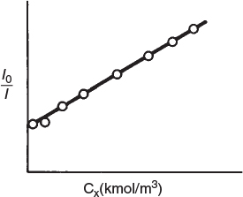
Example 9-1 The Stern–Volmer Equation

Light is given off when a high-intensity ultrasonic wave is applied to water.⁷ You should be able to see the glow if you turn out the lights and irradiate water with a focused ultrasonic tip. This light results from microsize gas bubbles (0.1 mm) being formed by the ultrasonic wave and then being compressed by it. During the compression stage of the wave, the contents of the bubble (e.g., water and whatever else is dissolved in the water, e.g., CS₂, O₂, N₂) are compressed adiabatically.

⁷ P. K. Chendke and H. S. Fogler, J. Phys. Chem., 87, 1362 (1983).

This compression gives rise to high temperatures and kinetic energies of the gas molecules, which through molecular collisions generate active intermediates and cause chemical reactions to occur in the bubble.

M + H_{2} O \to H_{2} O^{*} + M

$M + H_{2} O \to H_{2} O^{*} + M$

Collapsing cavitation microbubble

The intensity of the light given off, I, is proportional to the rate of deactivation of an activated water molecule that has been formed in the microbubble.

\begin{matrix} H_{2} O^{*} \overset{k}{\to} H_{2} O + hv \\ Light intensity (I)α(- r_{H_{2} O^{*}}) = k C_{H_{2} O^{*}} \end{matrix}

$\begin{matrix} H_{2} O^{*} \overset{k}{\to} H_{2} O + hv \\ Light intensity (I)α(- r_{H_{2} O^{*}}) = k C_{H_{2} O^{*}} \end{matrix}$

An order-of-magnitude increase in the intensity of sonoluminescence is observed when either carbon disulfide or carbon tetrachloride is added to the water. The intensity of luminescence, I, for the reaction is

C S_{2}^{*} \overset{k_{4}}{\to} {C S}_{2} + h v

$C S_{2}^{*} \overset{k_{4}}{\to} {C S}_{2} + h v$

Iα(- r_{C S_{2}^{*}}) = k_{4} C_{C S_{2}^{*}}

$Iα(- r_{C S_{2}^{*}}) = k_{4} C_{C S_{2}^{*}}$

A similar result exists for CCl₄.

However, when an aliphatic alcohol, X, is added to the solution, the intensity decreases with increasing concentration of alcohol. The data are usually reported in terms of a Stern–Volmer plot in which relative intensity is given as a function of alcohol concentration, C_X. (See Figure E9-1.1, where I₀ is the sonoluminescence intensity in the absence of alcohol and I is the sonoluminescence intensity in the presence of alcohol.)

(a) Suggest a mechanism consistent with experimental observation.

(b) Derive a rate law consistent with Figure E9-1.1.

Figure shows C subscript x (k moles per cubic meter) along the horizontal axis, ((l subscript 0) over l) axis along the vertical axis, and open dots that tend to rise from left to right are shown.

Figure E9-1.1 Ratio of luminescence intensities as a function of scavenger concentration.

Stern–Volmer plot

Solution

(a) Mechanism

From the linear plot we know that

\begin{matrix} \frac{I_{0}}{I} = A + B C_{X} \equiv A + B (X) & (E9-1.1) \end{matrix}

$\begin{matrix} \frac{I_{0}}{I} = A + B C_{X} \equiv A + B (X) & (E9-1.1) \end{matrix}$

where C_X ≡ (X) and A and B are numerical constants. Inverting Equation (E9-1.1) yields

\begin{matrix} \frac{I}{I_{0}} = \frac{1}{A + B (X)} & (E9-1.2) \end{matrix}

$\begin{matrix} \frac{I}{I_{0}} = \frac{1}{A + B (X)} & (E9-1.2) \end{matrix}$

From Rule 1 of Table 9-2, the denominator suggests that alcohol (X) collides with the active intermediate:

\begin{matrix} \begin{matrix} X+ Intermediate \to Deactivation products \end{matrix} & (E9-1 .3) \end{matrix}

$\begin{matrix} \begin{matrix} X+ Intermediate \to Deactivation products \end{matrix} & (E9-1 .3) \end{matrix}$

The alcohol acts as what is called a scavenger to deactivate the active intermediate. The fact that the addition of CCl₄ or CS₂ increases the intensity of the luminescence

\begin{matrix} I α ({CS}_{2}) & (E9-1 .4) \end{matrix}

$\begin{matrix} I α ({CS}_{2}) & (E9-1 .4) \end{matrix}$

Reaction pathways

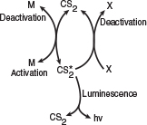
leads us to postulate (Rule 3 of Table 9-2) that the active intermediate ${CS}_{2}^{*}$ ${CS}_{2}^{*}$ was probably formed from the collision of either CS₂ or another gas M or both in the collapsing bubble

\begin{matrix} {M+ C S}_{2} \to {CS}_{2}^{*} + M & (E9-1.5) \end{matrix}

$\begin{matrix} {M+ C S}_{2} \to {CS}_{2}^{*} + M & (E9-1.5) \end{matrix}$

where M is a third body (CS₂, H₂O, N₂, etc.).

We also know that deactivation can occur by the reverse of reaction (E9-1.5). Combining this information, we have as our mechanism:

The mechanism

Activation: $\begin{matrix} {M+CS}_{2} \overset{k_{1}}{\to} {CS}_{2}^{*} + M & (E9-1.5) \end{matrix}$ $\begin{matrix} {M+CS}_{2} \overset{k_{1}}{\to} {CS}_{2}^{*} + M & (E9-1.5) \end{matrix}$

Deactivation: $\begin{matrix} M+ {CS}_{2}^{*} \overset{k_{2}}{\to} {CS}_{2} + M & (E9-1.6) \end{matrix}$ $\begin{matrix} M+ {CS}_{2}^{*} \overset{k_{2}}{\to} {CS}_{2} + M & (E9-1.6) \end{matrix}$

Deactivation: $\begin{matrix} M+ {CS}_{2}^{*} \overset{k_{3}}{\to} {CS}_{2} + X & (E9-1.3) \end{matrix}$ $\begin{matrix} M+ {CS}_{2}^{*} \overset{k_{3}}{\to} {CS}_{2} + X & (E9-1.3) \end{matrix}$

Luminescence: $\begin{matrix} {CS}_{2}^{*} \overset{k_{4}}{\to} {CS}_{2} + h v & (E9-1.7) \end{matrix}$ $\begin{matrix} {CS}_{2}^{*} \overset{k_{4}}{\to} {CS}_{2} + h v & (E9-1.7) \end{matrix}$

$\begin{matrix} {I=k}_{4} ({CS}_{2}^{*}) & (E 9 - 1.8) \end{matrix}$ $\begin{matrix} {I=k}_{4} ({CS}_{2}^{*}) & (E 9 - 1.8) \end{matrix}$

(b) Rate Law

Using the PSSH on $C S_{2}^{*}$ $C S_{2}^{*}$ in each of the above elementry reactions yields

r_{C S_{2}^{*}} = 0 = k_{1} ({CS}_{2}) (M) - k_{2} (C S_{2}^{*}) (M) - k_{3} (X) (C S_{2}^{*}) - k_{4} (C S_{2}^{*})

$r_{C S_{2}^{*}} = 0 = k_{1} ({CS}_{2}) (M) - k_{2} (C S_{2}^{*}) (M) - k_{3} (X) (C S_{2}^{*}) - k_{4} (C S_{2}^{*})$

Solving for ( $C S_{2}^{*}$ $C S_{2}^{*}$ ) and substituting into Equation (E9-1.8) gives us

Wolfram Sliders

\begin{matrix} I = \frac{k_{4} k_{1} (C S_{2}) (M)}{k_{2} (M) + k_{3} (X) + k_{4}} & (\begin{matrix} E9-1.9 \end{matrix}) \end{matrix}

$\begin{matrix} I = \frac{k_{4} k_{1} (C S_{2}) (M)}{k_{2} (M) + k_{3} (X) + k_{4}} & (\begin{matrix} E9-1.9 \end{matrix}) \end{matrix}$

In the absence of alcohol

\begin{matrix} I_{0} = \frac{k_{4} k_{1} (C S_{2}) (M)}{k_{2} (M) + k_{4}} & (\begin{matrix} E9-1.10 \end{matrix}) \end{matrix}

$\begin{matrix} I_{0} = \frac{k_{4} k_{1} (C S_{2}) (M)}{k_{2} (M) + k_{4}} & (\begin{matrix} E9-1.10 \end{matrix}) \end{matrix}$

For constant concentrations of CS₂ and the third body, M, we take a ratio of Equation (E9-1.10) to (E9-1.9)

$\begin{matrix} \frac{I_{0}}{I} = 1 + \frac{k_{3}}{k_{2} (M) + k_{4}} (X) = 1 + k^{'} (X) & (E 9 - 1.11) \end{matrix}$ $\begin{matrix} \frac{I_{0}}{I} = 1 + \frac{k_{3}}{k_{2} (M) + k_{4}} (X) = 1 + k^{'} (X) & (E 9 - 1.11) \end{matrix}$

which is of the same form as that suggested by Figure E9-1.1. Equation (E9-1.11) and similar equations involving scavengers are called Stern–Volmer equations.

Analysis: This example showed how to use the Rules of Thumb (Table 9-2) to develop a mechanism. Each step in the mechanism is assumed to follow an elementary rate law. The PSSH was applied to the net rate of reaction for the active intermediate in order to find the concentration of the active intermediate. This concentration was then substituted into the rate law for the rate of formation of product to give the rate law. The rate law from the mechanism was found to be consistent with experimental data.

A discussion of luminescence in the Web Module, Glow Sticks on the CRE Web site (www.umich.edu/~elements/5e/09chap/web.html). Here, the PSSH is applied to glow sticks. First, a mechanism for the reactions and luminescence is developed. Next, mole balance equations are written on each species and coupled with the rate law obtained using the PSSH; the resulting equations are solved and compared with experimental data.

Glow sticks Web Module

Steps in a chain reaction

9.1.4 Chain Reactions

A chain reaction consists of the following sequence:

1. Initiation: formation of an active intermediate

2. Propagation or chain transfer: interaction of an active intermediate with the reactant or product to produce another active intermediate

3. Termination: deactivation of the active intermediate to form products

Living Example Problem

An example comparing the application of the PSSH with the Polymath solution to the full set of equations is given in the Professional Reference Shelf R9.1, Chain Reactions, (http://www.umich.edu/~elements/5e/09chap/prof-chain.html). Also included in Professional Reference Shelf R9.2 is a discussion of Reaction Pathways and the chemistry of smog formation (http://www.umich.edu/~elements/5e/09chap/prof-rxnpath.html).

9.2 Enzymatic Reaction Fundamentals

An enzyme^† is a high-molecular-weight protein or protein-like substance that acts on a substrate (reactant molecule) to transform it chemically at a greatly accelerated rate, usually 10³ to 10¹⁷ times faster than the uncatalyzed rate. Without enzymes, essential biological reactions would not take place at a rate necessary to sustain life. Enzymes are usually present in small quantities and are not consumed during the course of the reaction, nor do they affect the chemical reaction equilibrium. Enzymes provide an alternate pathway for the reaction to occur, thereby requiring a lower activation energy. Figure 9-3 shows the reaction coordinate for the uncatalyzed reaction of a reactant molecule, called a substrate (S), to form a product (P)

† See http://www.rsc.org/Education/Teachers/Resources/cfb/enzymes.htm and https://en.wikipedia.org/wiki/Enzyme.

S → P

The figure also shows the catalyzed reaction pathway that proceeds through an active intermediate (E · S), called the enzyme–substrate complex, that is,

$S+E ⇄ E ·S \to E+P$ $S+E ⇄ E ·S \to E+P$

Because enzymatic pathways have lower activation energies, enhancements in reaction rates can be enormous, as in the degradation of urea by urease, where the degradation rate is on the order of 10¹⁴ higher than without the enzyme urease.

An important property of enzymes is that they are specific; that is, one enzyme can usually catalyze only one type of reaction. For example, a protease hydrolyzes only bonds between specific amino acids in proteins, an amylase works on bonds between glucose molecules in starch, and lipase attacks fats, degrading them to fatty acids and glycerol. Consequently, unwanted products are easily controlled in enzyme-catalyzed reactions. Enzymes are produced only by living organisms, and commercial enzymes are generally produced by bacteria. Enzymes usually work (i.e., catalyze reactions) under mild conditions: pH 4 to 9 and temperatures 75˚F to 160˚F. Most enzymes are named in terms of the reactions they catalyze. It is a customary practice to add the suffix -ase to a major part of the name of the substrate on which the enzyme acts. For example, the enzyme that catalyzes the decomposition of urea is urease and the enzyme that attacks tyrosine is tyrosinase. However, there are a few exceptions to the naming convention, such as a-amylase. The enzyme a-amylase catalyzes the transformation of starch in the first step in the production of the controversial soft drink (e.g., Red Pop) sweetener high-fructose corn syrup (HFCS) from corn starch, which is a $4 billion per year business.

Reaction coordinate for enzyme catalysis is depicted.

Figure 9-3 Reaction coordinate for enzyme catalysis.

\begin{matrix} Corn starch \overset{α - amylase}{\to} Thinned starch \to_{amylase}^{gluco -} Glucose \to_{isomerase}^{Glucose} HFCS \end{matrix}

$\begin{matrix} Corn starch \overset{α - amylase}{\to} Thinned starch \to_{amylase}^{gluco -} Glucose \to_{isomerase}^{Glucose} HFCS \end{matrix}$

9.2.1 Enzyme–Substrate Complex

The key factor that sets enzymatic reactions apart from other catalyzed reactions is the formation of an enzyme–substrate complex, (E · S). Here, substrate binds with a specific active site of the enzyme to form this complex.⁸ Figure 9-4 shows a schematic of the enzyme chymotrypsin (MW = 25,000 Daltons), which catalyzes the hydrolytic cleavage of polypeptide bonds. In many cases, the enzyme’s active catalytic sites are found where the various folds or loops interact. For chymotrypsin, the catalytic sites are noted by the amino acid numbers 57, 102, and 195 in Figure 9-4. Much of the catalytic power is attributed to the binding energy of the substrate to the enzyme through multiple bonds with the specific functional groups on the enzyme (amino side chains, metal ions). The type of interactions that stabilize the enzyme–substrate complex include hydrogen bonding and hydrophobic, ionic, and London van der Waals forces. If the enzyme is exposed to extreme temperatures or pH environments (i.e., both high and low pH values), it may unfold, losing its active sites. When this occurs, the enzyme is said to be denatured (see Figure 9.8 and Problem P9-13_B).

⁸ M. L. Shuler and F. Kargi, Bioprocess Engineering Basic Concepts, 2nd ed. (Upper Saddle River, NJ: Prentice Hall, 2002).

Figure shows a substrate represented by a molecule binds to a specific active site of an enzyme with the enzyme folded.

Graph shows the horizontal axis labeled "pH," the vertical axis labeled "rate." A bell shaped curve is shown touching the horizontal axis.

Schematic showing the loops and folds

Schematic of the enzyme chymotrypsin is shown with various loops and folds. Active sites are found at the interaction of folds or loops. A catalytic site Serine 195 is indicated. Disulfide bonds of the enzyme are also indicated.

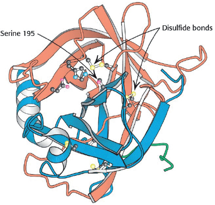
Figure 9-4 Enzyme chymotrypsin from Biochemistry, 7th ed., 2010 by Lubert Stryer, p. 258. Used with permission of W. H. Freeman and Company.

Two models for enzyme–substrate interactions are the lock-and-key model and the induced fit model, both of which are shown in Figure 9-5. For many years the lock-and-key model was preferred because of the sterospecific effects of one enzyme acting on one substrate. However, the induced fit model is the more useful model. In the induced fit model, both the enzyme molecule and the substrate molecules are distorted. These changes in conformation distort one or more of the substrate bonds, thereby stressing and weakening the bond to make the molecule more susceptible to rearrangement or attachment.

There are six classes of enzymes and only six:

1. Oxidoreductases	AH₂ + B + E → A + BH₂ + E
2. Transferases	AB + C + E → AC + B + E
3. Hydrolases	AB + H₂O + E → AH + BOH + E
4. Isomerases	A + E → isoA + E
5. Lyases	AB + E → A + B + E
6. Ligases	A + B + E → AB + E

More information about enzymes can be found on the following two Web sites: http://us.expasy.org/enzyme/ and www.chem.qmw.ac.uk/iubmb/enzyme. These sites also give information about enzymatic reactions in general.

9.2.2 Mechanisms

In developing some of the elementary principles of the kinetics of enzyme reactions, we shall discuss an enzymatic reaction that has been suggested by Levine and LaCourse as part of a system that would reduce the size of an artificial kidney.⁹ The desired result is a prototype of an artificial kidney that could be worn by the patient and would incorporate a replaceable unit for the elimination of the body’s nitrogenous waste products, such as uric acid and creatinine. A schematic of this device is shown in the CRE Web site (http://www.umich.edu/~elements/5e/09chap/summary.xhtml#sec2). In the microencapsulation scheme proposed by Levine and LaCourse, the enzyme urease would be used in the removal of urea from the bloodstream. Here, the catalytic action of urease would cause urea to decompose into ammonia and carbon dioxide. The mechanism of the reaction is believed to proceed by the following sequence of elementary reactions:

⁹ N. Levine and W. C. LaCourse, J. Biomed. Mater. Res., 1, 275.

Two models for the enzyme–substrate complex

In the lock-and-key model at the top, enzyme E with active site reacts with substrate S to form an enzyme-substrate complex in which the substrate fits exactly on the active site of the enzyme. The complex then forms enzyme E and two other different products P subscript 1 and P subscript 2. In the induced fit model at the bottom, enzyme E with active site reacts with substrate S to form an enzyme-substrate complex in which both the substrate molecule and the enzyme molecule are distorted to fit on the active site of the enzyme. The complex then forms enzyme E and two other different products P subscript 1 and P subscript 2. A micrograph below the induced fit model shows substrate (dextro-glucose) fitting into the active site of an enzyme with both the enzyme and the substrate distorted to make an induced fit.

Figure 9-5 Two models for enzyme–substrate interaction.

The reaction mechanism

1. The unbound enzyme urease (E) reacts with the substrate urea (S) to form an enzyme–substrate complex (E · S):

$\begin{matrix} N H_{2} C O N H_{2} + Urease \overset{k_{1}}{\to} [N H_{2} C O N H_{2} \cdot {Urease]}^{*} & (9-13) \end{matrix}$ $\begin{matrix} N H_{2} C O N H_{2} + Urease \overset{k_{1}}{\to} [N H_{2} C O N H_{2} \cdot {Urease]}^{*} & (9-13) \end{matrix}$

2. This complex (E · S) can decompose back to urea (S) and urease (E):

$\begin{matrix} [N H_{2} C O N H_{2} \cdot {Urease]}^{*} \overset{k_{2}}{\to} Urease + N H_{2} C O N {H_{2}}^{} & (9-14) \end{matrix}$ $\begin{matrix} [N H_{2} C O N H_{2} \cdot {Urease]}^{*} \overset{k_{2}}{\to} Urease + N H_{2} C O N {H_{2}}^{} & (9-14) \end{matrix}$

3. Or, it can react with water (W) to give the products (P) ammonia and carbon dioxide, and recover the enzyme urease (E):

\begin{matrix} [N H_{2} C O N H_{2} \cdot {Urease]}^{*} + H_{2} O \overset{k_{3}}{\to} {2NH}_{3} + {CO}_{2} + Urease & (9-15) \end{matrix}

$\begin{matrix} [N H_{2} C O N H_{2} \cdot {Urease]}^{*} + H_{2} O \overset{k_{3}}{\to} {2NH}_{3} + {CO}_{2} + Urease & (9-15) \end{matrix}$

S + E ⇆ E \cdot S \overset{+ H_{2} O}{\to} P + E

$S + E ⇆ E \cdot S \overset{+ H_{2} O}{\to} P + E$

Symbolically, the overall reaction is written as

S + E ⇆ E \cdot S \overset{+ H_{2} O}{\to} P + E

$S + E ⇆ E \cdot S \overset{+ H_{2} O}{\to} P + E$

We see that some of the enzyme added to the solution binds to the urea, and some of the enzyme remains unbound. Although we can easily measure the total concentration of enzyme, (E_t), it is difficult to measure either the concentration of free enzyme, (E), or the concentration of the bound enzyme (E · S).

Letting E, S, W, E · S, and P represent the enzyme, substrate, water, the enzyme–substrate complex, which is the active intermediate, and the reaction products, respectively, we can write Reactions (9-13), (9-14), and (9-15) symbolically in the forms

\begin{matrix} S + E \overset{k_{1}}{\to} E \cdot S & (9-16) \end{matrix}

$\begin{matrix} S + E \overset{k_{1}}{\to} E \cdot S & (9-16) \end{matrix}$

\begin{matrix} E \cdot S \overset{k_{2}}{\to} E + S & (9-17) \end{matrix}

$\begin{matrix} E \cdot S \overset{k_{2}}{\to} E + S & (9-17) \end{matrix}$

\begin{matrix} E \cdot S + W \overset{k_{3}}{\to} P + E & (9-18) \end{matrix}

$\begin{matrix} E \cdot S + W \overset{k_{3}}{\to} P + E & (9-18) \end{matrix}$

Here, P = 2NH₃ + CO₂.

The corresponding rate laws for Reactions (9-16), (9-17), and (9-18) are

\begin{matrix} r_{1 E \cdot S} = k_{1} (E) (S) & (9-16 A) \end{matrix}

$\begin{matrix} r_{1 E \cdot S} = k_{1} (E) (S) & (9-16 A) \end{matrix}$

\begin{matrix} r_{2 E \cdot S} = - k_{2} (E \cdot S) & (9-17 A) \end{matrix}

$\begin{matrix} r_{2 E \cdot S} = - k_{2} (E \cdot S) & (9-17 A) \end{matrix}$

\begin{matrix} r_{3 E \cdot S} = - k_{3} (E \cdot S) (W) & (9-18 A) \end{matrix}

$\begin{matrix} r_{3 E \cdot S} = - k_{3} (E \cdot S) (W) & (9-18 A) \end{matrix}$

where all the specific reaction rates are defined with respect to (E · S). The net rate of formation of product, r_P, is

$\begin{matrix} r_{P} = k_{3} (W) (E .S) & (9 - 19) \end{matrix}$ $\begin{matrix} r_{P} = k_{3} (W) (E .S) & (9 - 19) \end{matrix}$

For the overall reaction

E + S → P + E

we know that the rate of consumption of the urea substrate equals the rate of formation of product CO₂, i.e., –r_S = r_P.

This rate law, Equation (9-19), is of not much use to us in making reaction engineering calculations because we cannot measure the concentration of the active intermediate, which is the enzyme substrate complex (E · S). We will use the PSSH to express (E · S) in terms of measured variables.

The net rate of formation of the enzyme–substrate complex is

r_{E \cdot S} = r_{1 E \cdot S} + r_{2 E \cdot S} + r_{3 E \cdot S}

$r_{E \cdot S} = r_{1 E \cdot S} + r_{2 E \cdot S} + r_{3 E \cdot S}$

Substituting the rate laws, we obtain

\begin{matrix} r_{E \cdot S} = k_{1} (E) (S) - k_{2} (E \cdot S) - k_{3} (W) (E \cdot S) & (9-20) \end{matrix}

$\begin{matrix} r_{E \cdot S} = k_{1} (E) (S) - k_{2} (E \cdot S) - k_{3} (W) (E \cdot S) & (9-20) \end{matrix}$

Using the PSSH, r_E_·_S = 0, we can now solve Equation (9-20) for (E · S)

$\begin{matrix} (E .S) = \frac{k_{1} (E) (S)}{k_{2} + k_{3} (W)} & (9 - 21) \end{matrix}$ $\begin{matrix} (E .S) = \frac{k_{1} (E) (S)}{k_{2} + k_{3} (W)} & (9 - 21) \end{matrix}$

and substitute for (E · S) into Equation (9-19)

\begin{matrix} - r_{s} = r_{P} = \frac{k_{1} k_{3} (E) (S) (W)}{k_{2} + k_{3} (W)} & (9-22) \end{matrix}

$\begin{matrix} - r_{s} = r_{P} = \frac{k_{1} k_{3} (E) (S) (W)}{k_{2} + k_{3} (W)} & (9-22) \end{matrix}$

We need to replace unbound enzyme concentration (E) in the rate law.

We still cannot use this rate law because we cannot measure the unbound enzyme concentration (E); however, we can measure the total enzyme concentration, E_t.

In the absence of enzyme denaturation, the total concentration of the enzyme in the system, (E_t), is constant and equal to the sum of the concentrations of the free or unbounded enzyme, (E), and the enzyme–substrate complex, (E · S):

Total enzyme concentration = Bound + Free enzyme concentration.

\begin{matrix} (E_{t}) = (E) + (E \cdot S) & (9-23) \end{matrix}

$\begin{matrix} (E_{t}) = (E) + (E \cdot S) & (9-23) \end{matrix}$

Substituting for (E · S)

(E_{t}) = (E) + \frac{k_{1} (E) (S)}{k_{2} + k_{3} (W)}

$(E_{t}) = (E) + \frac{k_{1} (E) (S)}{k_{2} + k_{3} (W)}$

solving for (E)

(E) = \frac{(E_{t}) (k_{2} + k_{3} (W))}{k_{2} + k_{3} (W) + k_{1} (S)}

$(E) = \frac{(E_{t}) (k_{2} + k_{3} (W))}{k_{2} + k_{3} (W) + k_{1} (S)}$

and substituting for (E) in Equation (9-22), the rate law for substrate consumption is

$\begin{matrix} - r_{S} = \frac{k_{1} k_{3} (W) (E_{t}) (S)}{k_{1} (S) + k_{2} + k_{3} (W)} & (9 - 24) \end{matrix}$ $\begin{matrix} - r_{S} = \frac{k_{1} k_{3} (W) (E_{t}) (S)}{k_{1} (S) + k_{2} + k_{3} (W)} & (9 - 24) \end{matrix}$

Note: Throughout the following text, E_t ≡ (E_t) = total concentration of enzyme with typical units such as (kmol/m³) or (g/dm³).

9.2.3 Michaelis–Menten Equation

Because the reaction of urea and urease is carried out in an aqueous solution, water is, of course, in excess, and the concentration of water (W) is therefore considered constant, ca. 55 mol/dm³. Let

k_{c a t} = k_{3} (W) and let K_{M} = \frac{k_{c a t} + k_{2}}{k_{1}}

$k_{c a t} = k_{3} (W) and let K_{M} = \frac{k_{c a t} + k_{2}}{k_{1}}$

After dividing the numerator and denominator of Equation (9-24) by k₁, we obtain a form of the Michaelis–Menten equation:

\begin{matrix} - r_{S} = \frac{k_{c a t} (E_{t}) (S)}{(S) + K_{M}} & (9-25) \end{matrix}

$\begin{matrix} - r_{S} = \frac{k_{c a t} (E_{t}) (S)}{(S) + K_{M}} & (9-25) \end{matrix}$

The final form of the rate law

Turnover number k_cat

The parameter k_cat is also referred to as the turnover number. It is the number of substrate molecules converted to product in a given time on a single-enzyme molecule when the enzyme is saturated with substrate (i.e., all the active sites on the single-enzyme molecule are occupied, (S)>>K_M). For example, the turnover number for the decomposition of hydrogen-peroxide, H₂O₂, by the enzyme catalase is 40 × 10⁶ s^–1. That is, 40 million molecules of H₂O₂ are decomposed every second on a single-enzyme molecule saturated with H₂O₂. The constant K_M (mol/dm³) is called the Michaelis constant and for simple systems is a measure of the attraction of the enzyme for its substrate, so it’s also called the affinity constant. The Michaelis constant, K_M, for the decomposition of H₂O₂ discussed earlier is 1.1 M, while that for chymotrypsin is 0.1 M.¹⁰

¹⁰ D. L. Nelson and M. M. Cox, Lehninger Principles of Biochemistry, 3rd ed. (New York: Worth Publishers, 2000).

Michaelis constant K_M

If, in addition, we let V_max represent the maximum rate of reaction for a given total enzyme concentration

V_{\max} = k_{c a t} (E_{t})

$V_{\max} = k_{c a t} (E_{t})$

the Michaelis–Menten equation takes the familiar form

Michaelis–Menten equation

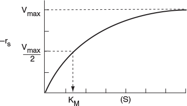
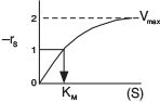
$\begin{matrix} - r_{S} = \frac{V_{\max} (S)}{K_{M} + (S)} & (9 - 26) \end{matrix}$ $\begin{matrix} - r_{S} = \frac{V_{\max} (S)}{K_{M} + (S)} & (9 - 26) \end{matrix}$

A sketch of the rate of disappearance of the substrate, –r_s, at a given concentration of total enzyme, E_T, is shown as a function of the substrate concentration, S, in Figure 9-6.

Graph shows the horizontal axis labeled (S), the vertical axis labeled negative r subscript S, and a concave downward curve.

Figure 9-6 Michaelis–Menten plot identifying the parameters V_max and K_M.

Michaelis–Menten plot

A plot of this type is sometimes called a Michaelis–Menten plot. At low substrate concentration, K_M ≫ (S), Equation (9-26) reduces to

- r_{s} ≅ \frac{V_{\max} (S)}{K_{M}}

$- r_{s} ≅ \frac{V_{\max} (S)}{K_{M}}$

and the reaction is apparent first order in the substrate concentration. At high substrate concentrations,

(S) ≫ K_{M}

$(S) ≫ K_{M}$

Equation (9-26) reduces to

- r_{s} ≅ V_{\max}

$- r_{s} ≅ V_{\max}$

Interpretation of Michaelis constant

and we see the reaction is apparent zero order.

What does K_M represent? Consider the case when the substrate concentration is such that the reaction rate is equal to one-half the maximum rate

- r_{s} = \frac{V_{\max}}{2}

$- r_{s} = \frac{V_{\max}}{2}$

then

$\begin{matrix} \frac{V_{\max}}{2} = \frac{V_{\max} (S_{1 / 2})}{K_{M} + (S_{1 / 2})} & (9-27) \end{matrix}$ $\begin{matrix} \frac{V_{\max}}{2} = \frac{V_{\max} (S_{1 / 2})}{K_{M} + (S_{1 / 2})} & (9-27) \end{matrix}$

Solving Equation (9-27) for the Michaelis constant yields

\begin{matrix} K_{M} = (S_{1 / 2}) & (9-28) \end{matrix}

$\begin{matrix} K_{M} = (S_{1 / 2}) & (9-28) \end{matrix}$

K_M = (S_1/2)

The Michaelis constant is equal to the substrate concentration at which the rate of reaction is equal to one-half the maximum rate, i.e., −r_A = V_max/2. The larger the value of K_M, the higher the substrate concentration necessary for the reaction rate to reach half of its maximum value.

The parameters V_max and K_M characterize the enzymatic reactions that are described by Michaelis–Menten kinetics. V_max is dependent on total enzyme concentration, whereas K_M is not.

Two enzymes may have the same values for k_cat but have different reaction rates because of different values of K_M. One way to compare the catalytic efficiencies of different enzymes is to compare their ratios k_cat/K_M. When this ratio approaches 10⁸ to 10⁹ (dm³/mol/s), the reaction rate approaches becoming diffusion limited. That is, it takes a long time for the enzyme and substrate to diffuse around in the fluid and find each other, but once they do they react immediately. We will discuss diffusion-limited reactions in Chapters 14 and 15.

Example 9-2 Evaluation of Michaelis–Menten Parameters V_max and K_M

In this example we illustrate how to determine the enzymatic reaction rate parameters V_max and K_M for the reaction rate.

\begin{matrix} Urea + Urease ⇄_{k_{2}}^{k_{1}} [Urea \cdot {Urease]}^{*} \to_{+ H_{2} O}^{k_{3}} 2 {NH}_{3} + {CO}_{2} + Urease \\ S+E ⇄E \cdot S \overset{+ H_{2} O}{\to} P + E \end{matrix}

$\begin{matrix} Urea + Urease ⇄_{k_{2}}^{k_{1}} [Urea \cdot {Urease]}^{*} \to_{+ H_{2} O}^{k_{3}} 2 {NH}_{3} + {CO}_{2} + Urease \\ S+E ⇄E \cdot S \overset{+ H_{2} O}{\to} P + E \end{matrix}$

The rate of reaction is given as a function of urea concentration in Table E9-2.1, where (S) ≡ C_urea.

TABLE E9-2.1 RATE DATA

C_urea (kmol/m³)	0.2	0.02	0.01	0.005	0.002
−r_urea (kmol/m³ · s)	1.08	0.55	0.38	0.2	0.09

(a) Determine the Michaelis–Menten parameters V_max and K_M for the reaction

(b) In addition to forming a Lineweaver–Burk Plot, form Hanes–Woolf and Eadie–Hofstee plots, and discuss the attributes of each type of plot.

Solution

Part (a)

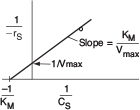
Inverting Equation (9-26) gives us the Lineweaver–Burk equation

\begin{matrix} \frac{1}{- r_{s}} = \frac{(S) + K_{M}}{V_{\max} (S)} = \frac{1}{V_{\max}} + \frac{K_{M}}{V_{\max}} \frac{1}{(S)} & \begin{matrix} (E9-2.1) \end{matrix} \end{matrix}

$\begin{matrix} \frac{1}{- r_{s}} = \frac{(S) + K_{M}}{V_{\max} (S)} = \frac{1}{V_{\max}} + \frac{K_{M}}{V_{\max}} \frac{1}{(S)} & \begin{matrix} (E9-2.1) \end{matrix} \end{matrix}$

Lineweaver–Burk equation

or in terms of urea

\begin{matrix} \frac{1}{- r_{urea}} = \frac{1}{V_{\max}} + \frac{K_{M}}{V_{max}} (\frac{1}{C_{urea}}) & (E9-2.2) \end{matrix}

$\begin{matrix} \frac{1}{- r_{urea}} = \frac{1}{V_{\max}} + \frac{K_{M}}{V_{max}} (\frac{1}{C_{urea}}) & (E9-2.2) \end{matrix}$

A plot of the reciprocal reaction rate versus the reciprocal urea concentration should be a straight line with an intercept (1/V_max) and slope (K_M/V_max). This type of plot is called a Lineweaver–Burk plot. We shall use the data in Table E9-2.2 to make two plots: a plot of –r_urea as a function of C_urea using Equation (9-26), which is called a Michaelis–Menten plot and is shown in Figure E9-2.1(a); and a plot of (1/–r_urea) as a function (1/C_urea), which is called a Lineweaver–Burk plot and is shown in Figure 9-2.1 (b).

Wolfram Sliders

TABLE E9-2.2 RAW AND PROCESSED DATA

C_urea (kmol/m³)	−r_urea (kmol/m³ · s)	1/C_urea (m³/kmol)	1/−r_urea (m³·s/kmol)
0.20	1.08	5.0	0.93
0.02	0.55	50.0	1.82
0.01	0.38	100.0	2.63
0.005	0.20	200.0	5.00
0.002	0.09	500.0	11.11

Graph shows (a) MichaelisMenten plot and (b) LineweaverBurk plot.

Figure E9-2.1 (a) Michaelis–Menten plot; (b) Lineweaver–Burk plot.

Michaelis–Menten Plot

Graph shows the horizontal axis labeled 1 over (C subscript S), the vertical axis labeled (1 over (negative r subscript S)), and a line.

Lineweaver–Burk Plot

Wolfram Sliders

The intercept on Figure E9-2.1(b) is 0.75, so

\frac{1}{V_{\max}} = 0.75 m^{3} \cdot s / kmol

$\frac{1}{V_{\max}} = 0.75 m^{3} \cdot s / kmol$

Therefore, the maximum rate of reaction is

V_max = 1.33 kmol/m³ · s = 1.33 mol/dm³ · s

From the slope, which is 0.02 s, we can calculate the Michaelis constant, K_M

\frac{K_{M}}{V_{max}} = slope = 0.02 s

$\frac{K_{M}}{V_{max}} = slope = 0.02 s$

Solving for K_M: K_M = 0.0266 kmol/m³.

For enzymatic reactions, the two key rate-law parameters are V_max and K_M.

Substituting K_M and V_max into Equation (9-26) gives us

\begin{matrix} - r_{urea} = \frac{1.33 C_{urea}}{0.0266 + C_{urea}} & (E9-2.3) \end{matrix}

$\begin{matrix} - r_{urea} = \frac{1.33 C_{urea}}{0.0266 + C_{urea}} & (E9-2.3) \end{matrix}$

where C_urea has units of (kmol/m³) and −r_urea has units of (kmol/m³ · s). Levine and LaCourse suggest that the total concentration of urease, (E_t), corresponding to the value of V_max above is approximately 5 g/dm³.

Part (b)

In addition to the Lineweaver–Burk plot, one can also use a Hanes–Woolf plot or an Eadie–Hofstee plot. Here, S ≡ C_urea, and –r_S ≡ –r_urea. Equation (9-26)

Eadie–Hofstee Plot

\begin{matrix} - r_{s} = \frac{V_{\max} (S)}{K_{M} + (S)} & (9-26) \end{matrix}

$\begin{matrix} - r_{s} = \frac{V_{\max} (S)}{K_{M} + (S)} & (9-26) \end{matrix}$

can be rearranged in the following forms. For the Eadie–Hofstee form

\begin{matrix} - r_{s} = V_{max} - K_{M} (\frac{- r_{S}}{(S)}) & (E9-2.4) \end{matrix}

$\begin{matrix} - r_{s} = V_{max} - K_{M} (\frac{- r_{S}}{(S)}) & (E9-2.4) \end{matrix}$

For the Hanes–Woolf form, we can rearrange Equation (9-26) to

\begin{matrix} \frac{(S)}{- r_{S}} = \frac{K_{M}}{V_{max}} + \frac{1}{V_{max}} (S) & (E9-2.5) \end{matrix}

$\begin{matrix} \frac{(S)}{- r_{S}} = \frac{K_{M}}{V_{max}} + \frac{1}{V_{max}} (S) & (E9-2.5) \end{matrix}$

Hanes–Woolf Plot

For the Eadie–Hofstee model, we plot –r_S as a function of [–r_S/(S)] and for the Hanes–Woolf model, we plot [(S)/–r_S] as a function of (S).

When to use the different models? The Eadie–Hofstee plot does not bias the data points at low substrate concentrations, while the Hanes–Woolf plot gives a more accurate evaluation of V_max. In Table E9-2.3, we add two columns to Table E9-2.1 to generate these plots (C_urea ≡ S).

Wolfram Sliders

TABLE E9-2.3 RAW AND PROCESSED DATA

S (kmol/m³)	–r_S (kmol/m³ · s)	1/S (m³/kmol)	1/–r_S (m³ · s/kmol)	S/–r_s (s)	–r_S/S (1/s)
0.20	1.08	5.0	0.93	0.185	5.4
0.02	0.55	50.0	1.82	0.0364	27.5
0.01	0.38	100.0	2.63	0.0263	38
0.005	0.20	200.0	5.00	0.0250	40
0.002	0.09	500.0	11.11	0.0222	45

The slope of the Hanes Woolf plot in Figure E9-2.2 (i.e., (1/ V_max) = 0.826 s · m³/kmol), gives V_max = 1.2 kmol/m³ · s and from the intercept, K_M/V_max = 0.02 s, we obtain K_M to be 0.024 kmol/m³.

Figure E9-2.2 Hanes–Woolf plot.

\frac{(S)}{- r_{S}} = \frac{K_{M}}{V_{\max}} + \frac{1 (S)}{V_{\max}}

$\frac{(S)}{- r_{S}} = \frac{K_{M}}{V_{\max}} + \frac{1 (S)}{V_{\max}}$

Hanes–Woolf plot

We next generate an Eadie–Hofstee plot form the data in Table E9-2.3. From the slope at the Eadie-Hofstee plot in Figure E9-2.3 (–0.0244 kmol/m³), we find K_M = 0.024 kmol/m³. Next, using the intercept at –r_S = 0, i.e., V_max/K_M = 50 s^–1, we calculate V_max = 1.22 kmol/m³ · s.

Figure E9-2.3 Eadie–Hofstee plot.

- r_{S} = V_{\max} - K_{M} (\frac{- r_{S}}{(S)})

$- r_{S} = V_{\max} - K_{M} (\frac{- r_{S}}{(S)})$

Eadie–Hofstee plot

Part (c) Regression

Equation (9-26) and Table E9-2.2 were used in the regression program of Polymath with the following results for V_max and K_M, as shown in Table E9-2.4.

TABLE E9-2.4 REGRESSION RESULTS

These values are within experimental error of those values of V_max and K_m deter-mined graphically.

Analysis: This example demonstrated how to evaluate the parameters V_max and K_M in the Michaelis–Menten rate law from enzymatic reaction data. Four techniques were used to evaluate V_max and K_M from experimental data: Lineweaver–Burk plot, Hanes–Woolf plot, Eadie–Hofstee plot, and non-linear regression. The advantage of each type of plot was discussed for evaluating the parameters V_max and K_M.

The Product-Enzyme Complex

In many reactions the enzyme and product complex (E · P) is formed directly from the enzyme substrate complex (E · S) according to the sequence

E + S ⇆ E \cdot S ⇆ P \cdot E ⇆ P + E

$E + S ⇆ E \cdot S ⇆ P \cdot E ⇆ P + E$

Briggs–Haldane Rate
Law

Applying the PSSH, after much effort and some approximations we obtain

\begin{matrix} - r_{s} = \frac{V_{\max} (C_{S} - C_{P} / K_{C})}{C_{S} + K_{\max} + K_{P} C_{P}} & (9-29) \end{matrix}

$\begin{matrix} - r_{s} = \frac{V_{\max} (C_{S} - C_{P} / K_{C})}{C_{S} + K_{\max} + K_{P} C_{P}} & (9-29) \end{matrix}$

which is often referred to as the Briggs–Haldane Equation [see P9-8_B (a)] and the application of the PSSH to enzyme kinetics, often called the Briggs–Haldane approximation.

9.2.4 Batch-Reactor Calculations for Enzyme Reactions

A mole balance on urea in a batch reactor gives

Mole balance

- \frac{d N_{u r e a}}{d t} = - r_{u r e a} V

$- \frac{d N_{u r e a}}{d t} = - r_{u r e a} V$

Because this reaction is liquid phase, V = V₀, the mole balance can be put in the following form:

\begin{matrix} - \frac{d C_{u r e a}}{d t} = - r_{u r e a} & (9-30) \end{matrix}

$\begin{matrix} - \frac{d C_{u r e a}}{d t} = - r_{u r e a} & (9-30) \end{matrix}$

The rate law for urea decomposition is

\begin{matrix} - r_{u r e a} = \frac{V_{\max} C_{u r e a}}{K_{M} + C_{u r e a}} & (9-31) \end{matrix}

$\begin{matrix} - r_{u r e a} = \frac{V_{\max} C_{u r e a}}{K_{M} + C_{u r e a}} & (9-31) \end{matrix}$

Rate law

Substituting Equation (9-31) into Equation (9-30) and then rearranging and integrating, we get

Combine

t = \int_{C_{u r e a}}^{C_{u r e a 0}} \frac{d C_{u r e a}}{- r_{u r e a}} = \int_{C_{u r e a}}^{C_{u r e a 0}} \frac{K_{M} + C_{u r e a}}{V_{\max} C_{u r e a}} d C_{u r e a}

$t = \int_{C_{u r e a}}^{C_{u r e a 0}} \frac{d C_{u r e a}}{- r_{u r e a}} = \int_{C_{u r e a}}^{C_{u r e a 0}} \frac{K_{M} + C_{u r e a}}{V_{\max} C_{u r e a}} d C_{u r e a}$

Integrate

\begin{matrix} t = \frac{K_{M}}{V_{\max}} ln \frac{C_{urea0}}{C_{urea}} + \frac{C_{urea0} - C_{urea}}{V_{\max}} & (9-32) \end{matrix}

$\begin{matrix} t = \frac{K_{M}}{V_{\max}} ln \frac{C_{urea0}}{C_{urea}} + \frac{C_{urea0} - C_{urea}}{V_{\max}} & (9-32) \end{matrix}$

We can write Equation (9-32) in terms of conversion as

C_urea = C_urea0 (1 – X)

\begin{matrix} t = \frac{K_{M}}{V_{\max}} ln \frac{1}{1 - X} + \frac{C_{urea0} X}{V_{\max}} & (9-32a) \end{matrix}

$\begin{matrix} t = \frac{K_{M}}{V_{\max}} ln \frac{1}{1 - X} + \frac{C_{urea0} X}{V_{\max}} & (9-32a) \end{matrix}$

Time to achieve a conversion X in a batch enzymatic reaction

The parameters K_M and V_max can readily be determined from batch-reactor data by using the integral method of analysis. Here, as shown in Figures 7-1, 7-2, and 7-3, we want to arrange our equation so that we can obtain a linear plot of our data. Letting S = C_urea and S₀ = C_urea0, we arrange Equation (9-32) in the form

\begin{matrix} \frac{1}{t} \ln \frac{S_{0}}{S} = \frac{V_{max}}{K_{M}} - \frac{S_{0} - S}{K_{M} t} & (9-33) \end{matrix}

$\begin{matrix} \frac{1}{t} \ln \frac{S_{0}}{S} = \frac{V_{max}}{K_{M}} - \frac{S_{0} - S}{K_{M} t} & (9-33) \end{matrix}$

The corresponding plot in terms of substrate concentration is shown in Figure 9-7.

Graph shows the intercept and slope of a line.

Figure 9-7 Evaluating V_max and K_M from batch-reactor data.

From Equation (9-33) we see that the slope of a plot of $[\frac{1}{t} \ln \frac{S_{0}}{S}]$ $[\frac{1}{t} \ln \frac{S_{0}}{S}]$ as a function of $[\frac{S_{0} - S}{t}]$ $[\frac{S_{0} - S}{t}]$ will be $(- \frac{1}{K_{m}})$ $(- \frac{1}{K_{m}})$ and the y intercept will be $(\frac{V_{\max}}{K_{m}})$ $(\frac{V_{\max}}{K_{m}})$ . In cases similar to Equation (9-33) where there is no possibility of confusion, we shall not bother to enclose the substrate or other species in parentheses to represent concentration [i.e., C_S ≡ (S) ≡ S].

Example 9-3 Batch Enzymatic Reactors

Calculate the time needed to convert 99% of the urea to ammonia and carbon dioxide in a 0.5-dm³ batch reactor. The initial concentration of urea is 0.1 mol/dm³, and the urease concentration is 0.001 g/dm³. The reaction is to be carried out isothermally at the same temperature at which the data in Table E9-2.2 were obtained.

Wolfram Sliders

Solution

We can use Equation (9-32)

\begin{matrix} t = \frac{K_{M}}{V_{\max}} \ln \frac{1}{1 - X} + \frac{C_{u r e a 0} X}{V_{\max}} & (9-32) \end{matrix}

$\begin{matrix} t = \frac{K_{M}}{V_{\max}} \ln \frac{1}{1 - X} + \frac{C_{u r e a 0} X}{V_{\max}} & (9-32) \end{matrix}$

From Table E9-2.3 we know K_M = 0.0233 mol / dm³, V_max = 1.2 mol / dm³ · s. The conditions given are X = 0.99 and C_ureao = 0.1 mol / dm³ (i.e., 0.1 kmol/m³). However, for the conditions in the batch reactor, the enzyme concentration is only 0.001 g/dm³, compared with 5 g/dm³ in Example 9-2. Because V_max = E_t · k₃, V_max for the second enzyme concentration is

\begin{matrix} V_{\max 2} = \frac{E_{t 2}}{E_{t 1}} V_{\max 1} = \frac{0.001}{5} \times 1.2 = 2.4 \times 1 0^{- 4} m o l / s \cdot d m^{3} \\ K_{M} = 0.0 233 m o l / d m^{3} and X = 0.99 \end{matrix}

$\begin{matrix} V_{\max 2} = \frac{E_{t 2}}{E_{t 1}} V_{\max 1} = \frac{0.001}{5} \times 1.2 = 2.4 \times 1 0^{- 4} m o l / s \cdot d m^{3} \\ K_{M} = 0.0 233 m o l / d m^{3} and X = 0.99 \end{matrix}$

Substituting into Equation (9-32)

\begin{matrix} t = & \frac{2.33 \times 10^{- 2} {mol/dm}^{3}}{2.4 \times 10^{- 4} {mol/dm}^{3} / s} 1 n (\frac{1}{0.01}) + \frac{(0.1 {mol/dm}^{3}) (0.99)}{2.4 \times 10^{- 4} {mol/dm}^{3} / s} \\ = & 447 s + 412 s \\ = & 859 s (14.325 min) \end{matrix}

$\begin{matrix} t = & \frac{2.33 \times 10^{- 2} {mol/dm}^{3}}{2.4 \times 10^{- 4} {mol/dm}^{3} / s} 1 n (\frac{1}{0.01}) + \frac{(0.1 {mol/dm}^{3}) (0.99)}{2.4 \times 10^{- 4} {mol/dm}^{3} / s} \\ = & 447 s + 412 s \\ = & 859 s (14.325 min) \end{matrix}$

Analysis: This example shows a straightforward Chapter 5–type calculation of the batch reactor time to achieve a certain conversion X for an enzymatic reaction with a Michaelis–Menten rate law. This batch reaction time is very short; consequently, a continuous-flow reactor might be better suited for this reaction.

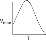
Effect of Temperature

The effect of temperature on enzymatic reactions is very complex. If the enzyme structure would remain unchanged as the temperature is increased, the rate would probably follow the Arrhenius temperature dependence. However, as the temperature increases, the enzyme can unfold and/or become denatured and lose its catalytic activity. Consequently, as the temperature increases, the reaction rate, –r_S, increases up to a maximum and then decreases as the temperature is increased further. The descending part of this curve is called temperature inactivation or thermal denaturizing.¹¹ Figure 9-8 shows an example of this optimum in enzyme activity.¹²

¹¹ M. L. Shuler and F. Kargi, Bioprocess Engineering Basic Concepts, 2nd ed. (Upper Saddle River, NJ: Prentice Hall, 2002), p. 77.

¹² S. Aiba, A. E. Humphrey, and N. F. Mills, Biochemical Engineering (New York: Academic Press, 1973), p. 47.

Graph shows the horizontal axis labeled T, the vertical axis labeled V subscript max, and a bell-shaped curve. The left end of the curve intersects the vertical axis and the right end of the curve tends to approach the horizontal axis.

9.3 Inhibition of Enzyme Reactions

In addition to temperature and solution pH, another factor that greatly influences the rates of enzyme-catalyzed reactions is the presence of an inhibitor. Inhibitors are species that interact with enzymes and render the enzyme either partially or totally ineffective to catalyze its specific reaction. The most dramatic consequences of enzyme inhibition are found in living organisms, where the inhibition of any particular enzyme involved in a primary metabolic pathway will render the entire pathway inoperative, resulting in either serious damage to or death of the organism. For example, the inhibition of a single enzyme, cytochrome oxidase, by cyanide will cause the aerobic oxidation process to stop; death occurs in a very few minutes. There are also beneficial inhibitors, such as the ones used in the treatment of leukemia and other neoplastic diseases. Aspirin inhibits the enzyme that catalyzes the synthesis of the module prostaglandin, which is involved in the pain-producing process. As shown in TV advertisements, the recent discovery of DDP-4 enzyme inhibitor Januvia has been approved for the treatment of Type 2 diabetes, a disease affecting 240 million people worldwide. Work Problem P9-15_C and then as the TV ad said, “Ask your doctor if Januvia is right for you.”

Graph shows a curve representing the Catalytic breakdown rate of H subscript 2 O subscript 2 depending on temperature.

Figure 9-8 Catalytic breakdown rate of H₂O₂ depending on temperature. Courtesy of S. Aiba, A. E. Humphrey, and N. F. Mills, Biochemical Engineering, Academic Press (1973).

The three most common types of reversible inhibition occurring in enzymatic reactions are competitive, uncompetitive, and noncompetitive. The enzyme molecule is analogous to a heterogeneous catalytic surface in that it contains active sites. When competitive inhibition occurs, the substrate and inhibitor are usually similar molecules that compete for the same site on the enzyme. Uncompetitive inhibition occurs when the inhibitor deactivates the enzyme–substrate complex, sometimes by attaching itself to both the substrate and enzyme molecules of the complex. Noncompetitive inhibition occurs with enzymes containing at least two different types of sites. The substrate attaches only to one type of site, and the inhibitor attaches only to the other to render the enzyme inactive.

9.3.1 Competitive Inhibition

Competitive inhibition is of particular importance in pharmacokinetics (drug therapy). If a patient were administered two or more drugs that react simultaneously within the body with a common enzyme, cofactor, or active species, this interaction could lead to competitive inhibition in the formation of the respective metabolites and produce serious consequences.

In competitive inhibition, another substance, i.e., I, competes with the substrate for the enzyme molecules to form an inhibitor–enzyme complex, as shown in Figure 9-9. That is, in addition to the three Michaelis–Menten reaction steps, there are two additional steps as the inhibitor (I) reversely ties up the enzyme, as shown in Reaction Steps 4 and 5.

The rate law for the formation of product in Reaction Step 3 is the same [cf. Equations (9-18A) and (9-19)] as it was before, i.e., in the absence of inhibitor

\begin{matrix} r_{P} = k_{3} (E \cdot S) & (9-34) \end{matrix}

$\begin{matrix} r_{P} = k_{3} (E \cdot S) & (9-34) \end{matrix}$

Reaction Steps

\begin{matrix} (1) & E + S \overset{k_{1}}{\to} E \cdot S \\ (2) & E \cdot S \overset{k_{2}}{\to} E + S \\ (3) & E \cdot S \overset{k_{3}}{\to} P + E \\ (4) & I + E \overset{k_{4}}{\to} E \cdot I (i n a c t i v e) \\ (5) & E \cdot I \overset{k_{5}}{\to} E + I \end{matrix}

$\begin{matrix} (1) & E + S \overset{k_{1}}{\to} E \cdot S \\ (2) & E \cdot S \overset{k_{2}}{\to} E + S \\ (3) & E \cdot S \overset{k_{3}}{\to} P + E \\ (4) & I + E \overset{k_{4}}{\to} E \cdot I (i n a c t i v e) \\ (5) & E \cdot I \overset{k_{5}}{\to} E + I \end{matrix}$

Competitive Inhibition Pathway

Figure 9-9 Competitive inhibition. Schematic drawing courtesy of Jofostan National Library, Lunčo, Jofostan, established 2019. New building completion expected in fall 2022.

Competitive inhibition pathway

Applying the PSSH, the net rate of reaction of the enzyme–substrate complex is

\begin{matrix} \begin{matrix} r_{E \cdot S} = 0 = k_{1} (E) (S) - k_{2} (E \cdot S) - k_{3} (E \cdot S) \end{matrix} & (9-35) \end{matrix}

$\begin{matrix} \begin{matrix} r_{E \cdot S} = 0 = k_{1} (E) (S) - k_{2} (E \cdot S) - k_{3} (E \cdot S) \end{matrix} & (9-35) \end{matrix}$

In a similar fashion, apply the PSSH to the net rate of formation of the inhibitor–substrate complex (E · I) is also zero

\begin{matrix} \begin{matrix} r_{E \cdot I} = 0 = k_{4} (E) (I) - k_{5} (E \cdot I) \end{matrix} & (9-36) \end{matrix}

$\begin{matrix} \begin{matrix} r_{E \cdot I} = 0 = k_{4} (E) (I) - k_{5} (E \cdot I) \end{matrix} & (9-36) \end{matrix}$

The total enzyme concentration is the sum of the bound and unbound enzyme concentrations

\begin{matrix} \begin{matrix} E_{t} = (E) + (E \cdot S) + (E \cdot I) \end{matrix} & (9-37) \end{matrix}

$\begin{matrix} \begin{matrix} E_{t} = (E) + (E \cdot S) + (E \cdot I) \end{matrix} & (9-37) \end{matrix}$

Combining Equations (9-35), (9-36), and (9-37), solving for (E · S) then substituting in Equation (9-34) and simplifying

\begin{matrix} r_{P} = - r_{S} = \frac{V_{max} (S)}{(S) + K_{M} (1 + \frac{(I)}{K_{I}})} & (9-38) \end{matrix}

$\begin{matrix} r_{P} = - r_{S} = \frac{V_{max} (S)}{(S) + K_{M} (1 + \frac{(I)}{K_{I}})} & (9-38) \end{matrix}$

Rate law for competitive inhibition

V_max and K_M are the same as before when no inhibitor is present; that is,

V_{\max} = k_{3} E_{t} and K_{M} = \frac{k_{2} + k_{3}}{k_{1}}

$V_{\max} = k_{3} E_{t} and K_{M} = \frac{k_{2} + k_{3}}{k_{1}}$

and the competitive inhibition constant K_I (mol/dm³) is defined as

K_{I} = \frac{k_{5}}{k_{4}}

$K_{I} = \frac{k_{5}}{k_{4}}$

By letting $K_{M}^{'} = K_{M} (1 + (I) / K_{I})$ $K_{M}^{'} = K_{M} (1 + (I) / K_{I})$ , we can see that the effect of adding a competitive inhibitor is to increase the “apparent” Michaelis constant, $K_{M}^{'}$ $K_{M}^{'}$ . A consequence of the larger “apparent” Michaelis constant $K_{M}^{'}$ $K_{M}^{'}$ is that a larger substrate concentration is needed for the rate of substrate decomposition, –r_S, to reach half its maximum rate.

Rearranging Equation (9-38) in order to generate a Lineweaver–Burk plot

\begin{matrix} \frac{1}{- r_{s}} = \frac{1}{V_{\max}} + \frac{1}{(S)} [\frac{K_{M}}{V_{\max}} (1 + \frac{(I)}{K_{I}})] & (9-39) \end{matrix}

$\begin{matrix} \frac{1}{- r_{s}} = \frac{1}{V_{\max}} + \frac{1}{(S)} [\frac{K_{M}}{V_{\max}} (1 + \frac{(I)}{K_{I}})] & (9-39) \end{matrix}$

From the Lineweaver–Burk plot (Figure 9-10), we see that as the inhibitor (I) concentration is increased, the slope increases (i.e., the rate decreases), while the intercept remains fixed.

Graph shows LineweaverBurk plot for competitive inhibition.

Figure 9-10 Lineweaver–Burk plot for competitive inhibition. (http://www.umich.edu/~elements/5e/09chap/live.html)

Wolfram Sliders

Side Note: Methanol Poisoning. An interesting and important example of competitive substrate inhibition is the enzyme alcohol dehydrogenase (ADH) in the presence of ethanol and methanol. If a person ingests methanol, ADH will convert it to formaldehyde and then formate, which causes blindness. Consequently, one treatment involves intravenously injecting ethanol (which is metabolized at a slower rate than methanol) at a controlled rate to tie up ADH to slow the metabolism of methanol to formaldehyde to formate so that the kidneys have time to filter out the methanol, which is then excreted in the urine. With this treatment, blindness may be avoided.

9.3.2 Uncompetitive Inhibition

Here, the inhibitor has no affinity for the enzyme by itself and thus does not compete with the substrate for the enzyme; instead, it ties up the enzyme–substrate complex by forming an inhibitor–enzyme–substrate complex, (I · E · S), which is inactive. In uncompetitive inhibition, the inhibitor reversibly ties up enzyme–substrate complex after it has been formed.

As with competitive inhibition, two additional reaction steps are added to the Michaelis–Menten kinetics for uncompetitive inhibition, as shown in Reaction Steps 4 and 5 in Figure 9-11.

Reaction Steps

\begin{matrix} (1) & E + S \overset{k_{1}}{\to} E \cdot S \\ (2) & E \cdot S \overset{k_{2}}{\to} E + S \\ (3) & E \cdot S \overset{k_{3}}{\to} P + E \\ (4) & I + E \cdot S \overset{k_{4}}{\to} I \cdot E \cdot S (i n a c t i v e) \\ (5) & I \cdot E \cdot S \overset{k_{5}}{\to} I+ E \cdot S \end{matrix}

$\begin{matrix} (1) & E + S \overset{k_{1}}{\to} E \cdot S \\ (2) & E \cdot S \overset{k_{2}}{\to} E + S \\ (3) & E \cdot S \overset{k_{3}}{\to} P + E \\ (4) & I + E \cdot S \overset{k_{4}}{\to} I \cdot E \cdot S (i n a c t i v e) \\ (5) & I \cdot E \cdot S \overset{k_{5}}{\to} I+ E \cdot S \end{matrix}$

Uncompetitive Pathway

Steps in uncompetitive enzyme inhibition are depicted.

Figure 9-11 Steps in uncompetitive enzyme inhibition.

Uncompetitive inhibition pathway

Starting with the equation for the rate of formation of product, Equation (9-34), and then applying the pseudo-steady-state hypothesis to the intermediate (I · E · S), we arrive at the rate law for uncompetitive inhibition

\begin{matrix} - r_{s} = r_{p} = \frac{V_{\max} (S)}{K_{M} + (S) (1 + \frac{(I)}{K_{I}})} {where K}_{I} = \frac{k_{5}}{k_{4}} & (9-40) \end{matrix}

$\begin{matrix} - r_{s} = r_{p} = \frac{V_{\max} (S)}{K_{M} + (S) (1 + \frac{(I)}{K_{I}})} {where K}_{I} = \frac{k_{5}}{k_{4}} & (9-40) \end{matrix}$

Rate law for uncompetitive inhibition

The intermediate steps are shown in the Chapter 9 Summary Notes in Learning Resources on the CRE Web site (http://www.umich.edu/~elements/5e/09chap/summary-example4.html).

Rearranging Equation (9-40)

\begin{matrix} \frac{1}{- r_{s}} = \frac{1}{(S)} \frac{K_{M}}{V_{max}} + \frac{1}{V_{max}} (1 + \frac{(I)}{K_{I}}) & (9-41) \end{matrix}

$\begin{matrix} \frac{1}{- r_{s}} = \frac{1}{(S)} \frac{K_{M}}{V_{max}} + \frac{1}{V_{max}} (1 + \frac{(I)}{K_{I}}) & (9-41) \end{matrix}$

The Lineweaver–Burk plot for uncompetitive enzyme inhibition is shown in Figure 9-12 for different inhibitor concentrations. The slope (K_M/V_max) remains the same as the inhibitor (I) concentration is increased, while the intercept [(1/V_max)(1 + (I)/K_I)] increases.

Graph shows LineweaverBurk plot for uncompetitive inhibition.

Figure 9-12 Lineweaver–Burk plot for uncompetitive inhibition.

9.3.3 Noncompetitive Inhibition (Mixed Inhibition)¹³

¹³ In some texts, mixed inhibition is a combination of competitive and uncompetitive inhibition.

In noncompetitive inhibition, also sometimes called mixed inhibition, the substrate and inhibitor molecules react with different types of sites on the enzyme molecule. Whenever the inhibitor is attached to the enzyme, it is inactive and cannot form products. Consequently, the deactivating complex (I · E · S) can be formed by two reversible reaction paths.

1. After a substrate molecule attaches to the enzyme molecule at the substrate site, then the inhibitor molecule attaches to the enzyme at the inhibitor site. (E • S + I ⇄ I • E • S)

2. After an inhibitor molecule attaches to the enzyme molecule at the inhibitor site, then the substrate molecule attaches to the enzyme at the substrate site. (E • I + S ⇄ I • E • S)

These paths, along with the formation of the product, P, are shown in Figure 9-13. In noncompetitive inhibition, the enzyme can be tied up in its inactive form either before or after forming the enzyme–substrate complex as shown in Steps 2, 3, and 4.

Again, starting with the rate law for the rate of formation of product and then applying the PSSH to the complexes (I · E) and (I · E · S), we arrive at the rate law for the noncompetitive inhibition

\begin{matrix} - r_{s} = \frac{V_{\max} (S)}{((S) + K_{M}) (1 + \frac{(I)}{K_{I}})} & (9-42) \end{matrix}

$\begin{matrix} - r_{s} = \frac{V_{\max} (S)}{((S) + K_{M}) (1 + \frac{(I)}{K_{I}})} & (9-42) \end{matrix}$

Rate law for noncompetitive inhibition

The derivation of the rate law is given in the Summary Notes on the CRE Web site (http://www.umich.edu/~elements/5e/09chap/summary-derive3.html). Equation (9-42) is in the form of the rate law that is given for an enzymatic reaction exhibiting noncompetitive inhibition. Heavy metal ions such as Pb²⁺, Ag⁺, and Hg²⁺, as well as inhibitors that react with the enzyme to form chemical derivatives, are typical examples of noncompetitive inhibitors.

Reaction Steps

\begin{matrix} (1) & E + S ⇄ E \cdot S \\ (2) & E + I ⇄ I \cdot E (inactive) \\ (3) & I + E \cdot S ⇄ I \cdot E \cdot S (inactive) \\ (4) & S + I \cdot E ⇄ I \cdot E \cdot S (inactive) \\ (5) & E \cdot S \to P + E \end{matrix}

$\begin{matrix} (1) & E + S ⇄ E \cdot S \\ (2) & E + I ⇄ I \cdot E (inactive) \\ (3) & I + E \cdot S ⇄ I \cdot E \cdot S (inactive) \\ (4) & S + I \cdot E ⇄ I \cdot E \cdot S (inactive) \\ (5) & E \cdot S \to P + E \end{matrix}$

Noncompetitive Pathway

Steps in noncompetitive enzyme inhibition are depicted.

Figure 9-13 Steps in noncompetitive enzyme inhibition.

Mixed inhibition

Rearranging Equation (9-42)

\begin{matrix} \frac{1}{- r_{s}} = \frac{1}{V_{max}} (1 + \frac{(I)}{K_{I}}) + \frac{1}{(S)} \frac{K_{M}}{V_{\max}} (1 + \frac{(I)}{K_{I}}) & (9-43) \end{matrix}

$\begin{matrix} \frac{1}{- r_{s}} = \frac{1}{V_{max}} (1 + \frac{(I)}{K_{I}}) + \frac{1}{(S)} \frac{K_{M}}{V_{\max}} (1 + \frac{(I)}{K_{I}}) & (9-43) \end{matrix}$

For noncompetitive inhibition, we see in Figure 9-14 that both the slope $(\frac{K_{M}}{V_{\max}} [1 + \frac{(I)}{K_{I}}])$ $(\frac{K_{M}}{V_{\max}} [1 + \frac{(I)}{K_{I}}])$ and intercept $(\frac{1}{V_{\max}} [1 + \frac{(I)}{K_{I}}])$ $(\frac{1}{V_{\max}} [1 + \frac{(I)}{K_{I}}])$ increase with increasing inhibitor concentration. In practice, uncompetitive inhibition and mixed inhibition are generally observed only for enzymes with two or more substrates, S₁ and S₂.

The three types of inhibition are compared with a reaction without inhibitors and are summarized on the Lineweaver–Burk plot shown in Figure 9-15.

In summary, we observe the following trends and relationships:

1. In competitive inhibition, the slope increases with increasing inhibitor concentration, while the intercept remains fixed.

2. In uncompetitive inhibition, the y-intercept increases with increasing inhibitor concentration, while the slope remains fixed.

3. In noncompetitive inhibition (mixed inhibition), both the y–intercept and slope will increase with increasing inhibitor concentration.

Graph shows LineweaverBurk plot for noncompetitive enzyme inhibition.

Figure 9-14 Lineweaver–Burk plot for noncompetitive enzyme inhibition.

Graph shows LineweaverBurk plot for three types of enzyme inhibition.

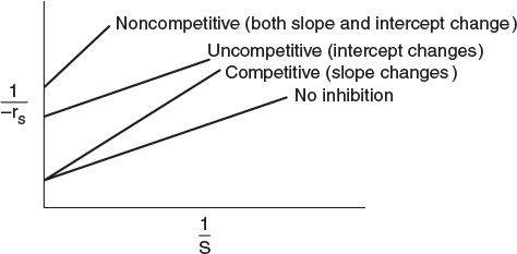
Figure 9-15 Summary: Lineweaver–Burk plots for three types of enzyme inhibition. (http://www.umich.edu/~elements/5e/09chap/live.html)

Summary plot of types of inhibition

Wolfram Sliders

Problem P9-12_B asks you to find the type of inhibition for the enzyme catalyzed reaction of starch.

9.3.4 Substrate Inhibition

In a number of cases, the substrate itself can act as an inhibitor, especially at high substrate concentrations. In the case of uncompetitive inhibition, the inactive molecule (S · E · S) is formed by the reaction

S + E · S → S · E · S (inactive)

Consequently, we see that by replacing (I) by (S) in Equation (9-40), the rate law for –r_S is

\begin{matrix} - r_{s} = \frac{V_{\max} (S)}{K_{M} + (S) + \frac{(S)^{2}}{K_{I}}} & (9-44) \end{matrix}

$\begin{matrix} - r_{s} = \frac{V_{\max} (S)}{K_{M} + (S) + \frac{(S)^{2}}{K_{I}}} & (9-44) \end{matrix}$

We see that at low substrate concentrations

\begin{matrix} K_{M} > > ((S) + \frac{(S)^{2}}{K_{I}}) & (9-45) \end{matrix}

$\begin{matrix} K_{M} > > ((S) + \frac{(S)^{2}}{K_{I}}) & (9-45) \end{matrix}$

then

\begin{matrix} - r_{s} ˜ \frac{V_{\max} (S)}{K_{M}} & (9-46) \end{matrix}

$\begin{matrix} - r_{s} ˜ \frac{V_{\max} (S)}{K_{M}} & (9-46) \end{matrix}$

and the rate increases linearly with increasing substrate concentration.

At high substrate concentrations ((S)² / K_I) >>(K_M + (S)), then

\begin{matrix} - r_{S} = \frac{V_{\max} K_{I}}{S} & (9-47) \end{matrix}

$\begin{matrix} - r_{S} = \frac{V_{\max} K_{I}}{S} & (9-47) \end{matrix}$

Substrate inhibition

and we see that the rate decreases as the substrate concentration increases. Consequently, the rate of reaction goes through a maximum in the substrate concentration, as shown in Figure 9-16. We also see that there is an optimum substrate concentration at which to operate. This maximum is found by setting the derivative of –r_S wrt S in Equation (9-44) equal to 0, to obtain

\begin{matrix} S_{max} = \sqrt{K_{M} K_{I}} & (9-48) \end{matrix}

$\begin{matrix} S_{max} = \sqrt{K_{M} K_{I}} & (9-48) \end{matrix}$

When substrate inhibition is possible, the substrate is fed to a semibatch reactor called a fed batch to maximize the reaction rate and conversion.

Graph shows Substrate reaction rate as a function of substrate concentration for substrate inhibition.

Figure 9-16 Substrate reaction rate as a function of substrate concentration for substrate inhibition.

Our discussion of enzymes is continued in the Professional Reference Shelf on the CRE Web site where we describe multiple enzyme and substrate systems, enzyme regeneration, and enzyme co-factors (see R9.6; http://www.umich.edu/~elements/5e/09chap/prof-07prof2.html

..................Content has been hidden....................

You can't read the all page of ebook, please click here login for view all page.

Table of Contents for Chapter 9 Reaction Mechanisms, Pathways, Bioreactions, and Bioreactors

Create new playlist

Sign In

Sign Up

9. Reaction Mechanisms, Pathways, Bioreactions, and Bioreactors

9.1 Active Intermediates and Nonelementary Rate Laws

9.1.1 Pseudo-Steady-State Hypothesis (PSSH)

9.1.2 If Two Molecules Must Collide, How Can the Rate Law Be First Order?

9.1.3 Searching for a Mechanism

9.1.4 Chain Reactions

9.2 Enzymatic Reaction Fundamentals

9.2.1 Enzyme–Substrate Complex

9.2.2 Mechanisms

9.2.3 Michaelis–Menten Equation

The Product-Enzyme Complex

9.2.4 Batch-Reactor Calculations for Enzyme Reactions

Effect of Temperature

9.3 Inhibition of Enzyme Reactions

9.3.1 Competitive Inhibition

9.3.2 Uncompetitive Inhibition

9.3.3 Noncompetitive Inhibition (Mixed Inhibition)13

9.3.4 Substrate Inhibition

Table of Contents for
Chapter 9 Reaction Mechanisms, Pathways, Bioreactions, and Bioreactors

9.3.3 Noncompetitive Inhibition (Mixed Inhibition)¹³