12.5.2 Heat-GeneratedTerm,G(T)

Search in book...
Toggle Font Controls
Create new playlist

Name your new playlist

Playlist description (optional)
Sign In

Email address

Password

Forgot Password?

or

Continue with Facebook

Continue with Google
Sign Up

Full Name

Email address

Confirm Email Address

Password

or

Continue with Facebook

Continue with Google

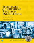
Vary Non-adiabatic Parameter κ. If one increases κ by either decreasing the molar flow rate, F_A0, or increasing the heat-exchange area, A, the slope increases and for the case of T_a < T₀ the ordinate intercept moves to the left, as shown in Figure 12-8.

Graph depicts variation of heat-removed line with kappa.

Figure 12-8 Variation of heat-removed line with κ (κ = UA/C_P0F_A0).

κ=UACP0FA0Tc=T0+κTa1+κ $\begin{matrix} κ = \frac{U A}{C_{P0} F_{A0}} \\ T_{c} = \frac{T_{0} + κ T_{a}}{1 + κ} \end{matrix}$

κ = 0 κ = \infty T c = T 0 T c = T a

$\begin{matrix} κ = 0 & T_{c} = T_{0} \\ κ = \infty & T_{c} = T_{a} \end{matrix}$

On the other hand, if T_a > T₀, the intercept will move to the right as κ increases.

12.5.2 Heat-Generated Term, G(T)

The heat-generated term, Equation (12-29), can be written in terms of conversion. [Recall that X = −r_AV/F_A0.]

G (T) = (- Δ H o R x) X (12-31)

$\begin{matrix} G (T) = (- Δ H_{R x}^{o}) X & \begin{matrix} (12-31) \end{matrix} \end{matrix}$

To obtain a plot of heat generated, G(T), as a function of temperature, we must solve for X as a function of T using the CSTR mole balance, the rate law, and stoichiometry. For example, for a first-order liquid-phase reaction, the CSTR mole balance becomes

V = F A 0 X k C A = v 0 C A 0 X k C A 0 ( 1 - X )

$V = \frac{F_{A 0} X}{k C_{A}} = \frac{v_{0} C_{A 0} X}{k C_{A 0} (1 - X)}$

Solving for X yields

First-order reaction

X = τ k 1 + τ k (5-8)

$\begin{matrix} X = \frac{τ k}{1 + τ k} & \begin{matrix} (5-8) \end{matrix} \end{matrix}$

Substituting for X in Equation (12-31), we obtain

G (T) = - Δ H o R x τ k 1 + τ k (12-32)

$\begin{matrix} G (T) = \frac{- Δ H_{R x}^{o} τ k}{1 + τ k} & \begin{matrix} (12-32) \end{matrix} \end{matrix}$

Finally, substituting for k in terms of the Arrhenius equation, we obtain

G(T)=−ΔH∘RxτAe−E/RT1+τAe−E/Rt(12−33) $\begin{matrix} G (T) = \frac{- Δ H_{Rx}^{\circ} τ A e^{- E / R T}}{1 + τ A e^{- E / R t}} & \begin{matrix} (12 - 33) \end{matrix} \end{matrix}$

Second-order reaction

Note that equations analogous to Equation (12-33) for G (T) can be derived for other reaction orders and for reversible reactions simply by solving the CSTR mole balance for X. For example, for the second-order liquid-phase reaction

X = ( 2 τ k C A 0 + 1 ) - 4 τ k C A 0 + 1 - - - - - - - - \sqrt 2 τ k C A 0

$X = \frac{(2 τ k C_{A 0} + 1) - \sqrt{4 τ k C_{A 0} + 1}}{2 τ k C_{A 0}}$

the corresponding heat generated term is

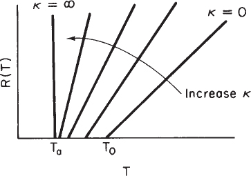
G(T)=−ΔH∘Rx[(2τCA0Ae−E/RT+1)−4τCA0Ae−E/RT+1√]2τCA0Ae−E/RT(12−34) $\begin{matrix} G (T) = \frac{- Δ H_{Rx}^{\circ} [(2 τ C_{A0} {A e}^{- E / R T} + 1) - \sqrt{4 τ C_{A0} A e^{- E / R T} + 1}]}{2 τ C_{A0} A e^{- E / R T}} & \begin{matrix} (12 - 34) \end{matrix} \end{matrix}$

Let’s now return to our first-order reaction, Equation (12-33), and examine the behavior of the G(T) curve. At very low temperatures, the second term in the denominator of Equation (12-33) for the first-order reaction can be neglected, so that G(T) varies as

Low T

G (T) = - Δ H o R x τ A e - E / R T

$G (T) = - Δ H_{R x}^{o} τ A e^{- E / R T}$

(Recall that ΔHoRx $Δ H_{R x}^{o}$ means that the standard heat of reaction is evaluated at T_R.)

At very high temperatures, the second term on the right side in the denominator dominates in Equation (12-33) so that the τk in the numerator and denominator cancel, and G(T) is reduced to

High T

G (T) = - Δ H o R x

$G (T) = - Δ H_{R x}^{o}$

G(T) is shown as a function of T for two different activation energies, E, in Figure 12-9. If the flow rate is decreased or the reactor volume increased so as to increase τ, the heat-generated term, G(T ), changes, as shown in Figure 12-10.

Graph depicts variation of G(T) curve with activation energy.

Figure 12-9 Variation of G(T) curve with activation energy.

Graph depicts variation of G(T) curve with space time.

Figure 12-10 Variation of G(T) curve with space time.

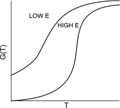
Heat-generated curves, G (T)

Can you combine Figures 12-10 and 12-8 to explain why a Bunsen burner goes out when you turn up the gas flow to a very high rate?

12.5.3 Ignition-Extinction Curve

The points of intersection of R(T) and G(T) give us the temperature at which the reactor can operate at steady state. This intersection is the point at which both the energy balance, R(T), and the mole balance, G(T), are satisfied. Suppose that we begin to feed our reactor at some relatively low temperature, T₀₁. If we construct our G(T) and R(T) curves, illustrated by curve y = G(T) and line a = R(T), respectively, in Figure 12-11, we see that there will be only one point of intersection, point 1. From this point of intersection, one can find the steady-state temperature in the reactor, T_s1, by following a vertical line down to the T-axis and reading off the temperature, T_s1, as shown in Figure 12-11.

Graph depicts multiple intersecting points with temperature varied.

Figure 12-11 Finding multiple steady states with T₀ varied.

If one were now to increase the entering temperature to T₀₂, the G(T) curve, y, would remain unchanged, but the R(T) curve would move to the right, as shown by line b in Figure 12-11, and will now intersect the G(T) at point 2 and be tangent at point 3. Consequently, we see from Figure 12-11 that there are two steady-state temperatures, T_s2 and T_s3, that can be realized in the CSTR for an entering temperature T₀₂. If the entering temperature is increased to T₀₃, the R(T) curve, line c (Figure 12-12), intersects the G(T) curve three times and there are three steady-state temperatures, T_s4, T_s5, and T_s6. As we continue to increase T₀, we finally reach line e, in which there are only two steady-state temperatures, a point of tangency at T_s10 and an intersection at T_s11. If the entering temperature is slightly increased beyond T₀₅, say to T₀₆, then there is a jump in reactor temperature, from T_s10 up to T_s12. This jump is called the ignition point for the reaction. By further increasing T₀, we reach line f, corresponding to T₀₆, in which we have only one reactor temperature that will satisfy both the mole and energy balances, T_s12. For the six entering temperatures, we can form Table 12-4, relating the entering temperature to the possible reactor operating temperatures.

Both the mole and energy balances are satisfied at the points of intersection or tangency.

Graph depicts multiple intersecting points with entering temperature varied.

The horizontal axis represents T and the vertical axis represents R(T), G(T). Six slanting parallel lines from a to f are drawn from left to right with the slanting lines meeting the horizontal axis at T subscript 01, T subscript 02, T subscript 03, T subscript 04, T subscript 05, and T subscript 06, respectively, from left to right. A curve is drawn starting from the bottom of the vertical axis, increasing gradually initially, increasing vertically upward in the middle, and then again increasing gradually. Line a intersects with the curve at point 1 at the bottom of the line. Line b intersects with point 2 at the bottom and be tangent with point 3 at the top. Line c intersects with the curve at points 4, 5, and 6 from bottom to top. Line d intersects with the curve at points 7, 8, and 9 from bottom to top. Line e is tangent with point 10 at the bottom and intersects with point 11 at the top. Line f intersects with point 12 at the top.

Figure 12-12 Finding multiple steady states with T₀ varied.

Table 12-4 Multiple Steady-State Temperatures

Entering Temperature	Reactor Temperatures
T₀₁			T_s1
T₀₂		T_s2		T_s3
T₀₃	T_s4		T_s5		T_s6
T₀₄	T_s7		T_s8		T_s9
T₀₅		T_s10		T_s11
T₀₆			T_s12

By plotting steady-state reactor temperature T_s as a function of entering temperature T₀, we obtain the well-known ignition-extinction curve shown in Figure 12-13. From this figure, we see that as the entering temperature T₀ is increased, the steady-state temperature T_s increases along the bottom line until T₀₅ is reached. Any fraction-of-a-degree increase in temperature beyond T₀₅ and the steady-state reactor temperature T_s will jump up from T_s10 to T_s11, as shown in Figure 12-13. The temperature at which this jump occurs is called the ignition temperature. That is, we must exceed a certain feed temperature, T₀₅, to operate at the upper steady state where the temperature and conversion are higher.

Graph depicts temperature ignition-extinction curve.

The horizontal axis representing entering temperature T subscript 0 is marked as T subscript 01, T subscript 02, T subscript 03, T subscript 04, T subscript 05, and T subscript 06 from left to right. The vertical axis representing Reactor Temperature T subscript S is marked as T subscript S1 at the bottom and T subscript S6 at the top. A line connecting the points 1, 2, 4, 7, and 10 above T subscript 01, T subscript 02, T subscript 03, T subscript 04, and T subscript 05, respectively, of the horizontal axis is indicated as lower steady states. A vertical line is drawn from point 10 to point 11 above it with point 10 indicated as ignition temperature. A line from point 12 above T subscript 06 of the horizontal axis drawn through the points 11, 9, 6, and 3 is indicated as upper steady states. A vertical line is drawn from point 3 to point 2 with point 2 indicated as extinction temperature. A dotted line from point 3 to point 10 through points 5 and 8 is indicated as unstable steady states.

Figure 12-13 Temperature ignition-extinction curve.

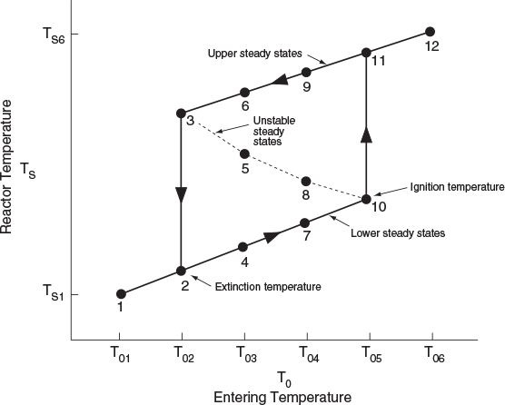
If a reactor were operating at T_s12 and we began to cool the entering temperature down from T₀₆, the steady-state reactor temperature, T_s3, would eventually be reached, corresponding to an entering temperature, T₀₂. Any slight decrease below T₀₂ would drop the steady-state reactor temperature to immediately the lower steady-state value T_s2 . Consequently, T₀₂ is called the extinction temperature.

The middle points 5 and 8 in Figures 12-12 and 12-13 represent unstable steady-state temperatures. Consider the heat-removed line d in Figure 12-12, along with the heat-generated curve y, which are replotted in Figure 12-14. If we were operating at the middle steady-state temperature T_s8, for example, and a pulse increase in reactor temperature occurred, we would find ourselves at the temperature shown by vertical line ②, between points 8 and 9. We see that along this vertical line ②, the heat-generated curve, y ≡ G(T), is greater than the heat-removed line d ≡ R(T) i.e., (G > R). Consequently, the temperature in the reactor would continue to increase until point 9 is reached at the upper steady state. On the other hand, if we had a pulse decrease in temperature from point 8, we would find ourselves on a vertical line ③ between points 7 and 8. Here, we see that the heat-removed curve d is greater than the heat-generated curve y (R > G), so the temperature will continue to decrease until the lower steady state is reached. That is, a small change in temperature either above or below the middle steady-state temperature, T_s8, will cause the reactor temperature to move away from this middle steady state. Steady states that behave in this manner are said to be unstable.

Graph depicts stability of multiple steady state temperatures.

The horizontal axis represents T and the vertical axis represents R(T), G(T). A slanting line d meets the horizontal axis at T subscript 04. Curve y intersects with line d at points 7, 8, and 9. Vertical lines through points 7, 8, and 9 meet the horizontal axis at T subscript S7, T subscript S8, and T subscript S9, respectively. Curve y is above line d before T subscript S7, below line d between T subscript S7 and T subscript S8, above line d between T subscript S8 and T subscript S9, and below line d after T subscript S9. G is greater than R before the vertical line from T subscript S7. R is greater than G between the vertical lines from T subscript S7 and T subscript S8. G is greater than R between the vertical lines from T subscript S8 and T subscript S9. R is greater than G after the vertical line from T subscript S9. Vertical line 4 is drawn to the left of point 7. Vertical line 3 is drawn to the left of point 8. Vertical line 2 is drawn between points 8 and 9. Vertical line 1 is drawn to the right of point 9.

Figure 12-14 Stability of multiple steady state temperatures.

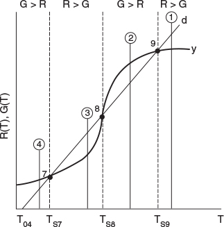
In contrast to these unstable operating points, there are stable operating points. Consider what would happen if a reactor operating at T_s9 were subjected to a pulse increase in reactor temperature indicated by line ① in Figure 12-14. We see that the heat-removed line d is greater than the heat-generated curve y (R > G), so that the reactor temperature will decrease and return to T_s9. On the other hand, if there is a sudden drop in temperature below T_s9, as indicated by line ②, we see the heat-generated curve y is greater than the heat-removed line d (G > R), and the reactor temperature will increase and return to the upper steady state at T_s9. Consequently, T_s9 is a stable steady state.

Next, let’s look at what happens when the lower steady-state temperature at T_s7 is subjected to pulse increase to the temperature shown as line ③ in Figure 12-14. Here, we again see that the heat removed, R, is greater than the heat generated, G, so that the reactor temperature will drop and return to T_s7. If there is a sudden decrease in temperature below T_s7 to the temperature indicated by line ④, we see that the heat generated is greater than the heat removed (G > R), and that the reactor temperature will increase until it returns to T_s7. Consequently, T_s7 is a stable steady state. A similar analysis could be carried out for temperatures T_s1, T_s2, T_s4, T_s6, T_s11, and T_s12, and one would find that reactor temperatures would always return to locally stable steady-state values when subjected to both positive and negative fluctuations.

While these points are locally stable, they are not necessarily globally stable. That is, a large perturbation in temperature or concentration may be sufficient to cause the reactor to fall from the upper steady state (corresponding to high conversion and temperature, such as point 9 in Figure 12-14), to the lower steady state (corresponding to low temperature and conversion, point 7).

12.6 Nonisothermal Multiple Chemical Reactions

Most reacting systems involve more than one reaction and do not operate iso-thermally. This section is one of the most important, if not the most important, sections of the book. It ties together all the previous chapters to analyze multiple reactions that do not take place isothermally.

12.6.1 Energy Balance for Multiple Reactions in Plug-Flow Reactors

Energy balance for multiple reactions

In this section we give the energy balance for multiple reactions. We begin by recalling the energy balance for a single reaction taking place in a PFR, which is given by Equation (12-5)

d T d V = ( - r A ) [ - Δ H R x ( T ) ] - U a ( T - T a ) Σ j = 1 m F j C P j (12-5)

$\begin{matrix} \frac{d T}{d V} = \frac{(- r_{A}) [- Δ H_{R x} (T)] - U a (T - T_{a})}{Σ_{j = 1}^{m} F_{j} C_{P_{j}}} & \begin{matrix} (12-5) \end{matrix} \end{matrix}$

When we have multiple reactions occurring, we have to account for, and sum up, all the heats of reaction in the reactor for each and every reaction. For q multiple reactions taking place in a PFR where there are m species, it is easily shown that Equation (12-5) can be generalized to (cf. P12-1(j))

i = Reaction number

j = Species

dTdV=Σi=1q(−rij)[−ΔHRxij(T)]−Ua(T−Ta)Σj=1mFjCPj(12−35) $\begin{matrix} \frac{d T}{d V} = \frac{Σ_{i = 1}^{q} (- r_{i j}) [- Δ H_{Rx i j} (T)] - U a (T - T_{a})}{Σ_{j = 1}^{m} F_{j} C_{P_{j}}} & \begin{matrix} (12 - 35) \end{matrix} \end{matrix}$

Note that we now have two subscripts on the heat of reaction. The heat of reaction for reaction i must be referenced to the same species in the rate, r_ij, by which ΔH_Rxij. is multiplied, which is

[−rij][−ΔHRxij]=[Moles ofj reacted in reaction iVolume⋅time]×[joules "released" in reaction iMoles ofj reacted in reaction i]=[Joules "released" in reaction iVolume⋅time](12−36) $\begin{matrix} \begin{matrix} [- r_{i j}] [- Δ H_{Rx i j}] & = [\frac{Moles of j reacted in reaction i}{Volume \cdot time}] \times [\frac{joules "released" in reaction i}{Moles of j reacted in reaction i}] \\ = [\frac{Joules "released" in reaction i}{Volume \cdot time}] \end{matrix} & \begin{matrix} (12 - 36) \end{matrix} \end{matrix}$

where the subscript j refers to the species, the subscript i refers to the particular reaction, q is the number of independent reactions, and m is the number of species. We are going to let

Qg=Σi=1q(−rij)[−ΔHRxij(T)] $Q_{g} = Σ_{i = 1}^{q} (- r_{i j}) [- Δ H_{Rx i j} (T)]$

and

Qr=Ua(T−Ta) $Q_{r} = U a (T - T_{a})$

Then Equation (12-35) becomes

dTdV=Qg−QrΣj=1mFjCPj(12−37) $\begin{matrix} \frac{d T}{d V} = \frac{Q_{g} - Q_{r}}{Σ_{j = 1}^{m} F_{j} C_{P_{j}}} & \begin{matrix} (12 - 37) \end{matrix} \end{matrix}$

Equation (12-37) represents a nice compact form of the energy balance for multiple reactions.

Consider the following reaction sequence carried out in a PFR:

One of the major goals of this text is that the reader will be able to solve multiple reactions with heat effects, and this section shows how!

Reaction 1:Reaction 2:A−→−−−k1BB−→−−−k2C $\begin{matrix} Reaction 1: & A \overset{k_{1}}{\to} B \\ Reaction 2: & B \overset{k_{2}}{\to} C \end{matrix}$

The PFR energy balance becomes

Q g Q r = = (- Δ H R x 1 A) (- r 1 A) + (- r 2 B) (- Δ H R x 2 B) U a (T - T a)

$\begin{matrix} Q_{g} & = & (- Δ H_{R x 1 A}) (- r_{1 A}) + (- r_{2 B}) (- Δ H_{R x 2 B}) \\ Q_{r} & = & U a (T - T_{a}) \end{matrix}$

Substituting for Q_g and -Q_r in Equation (12-37) we obtain

d T d V = U a ( T a - T ) + ( - r 1 A ) ( - Δ H R x 1 A ) + ( - r 2 B ) ( - Δ H R x 2 B ) F A C P A + F B C P B + F C C P C (12-38)

$\begin{matrix} \frac{d T}{d V} = \frac{U a (T_{a} - T) + (- r_{1 A}) (- Δ H_{R x 1 A}) + (- r_{2 B}) (- Δ H_{R x 2 B})}{F_{A} C_{P_{A}} + F_{B} C_{P_{B}} + F_{C} C_{P_{C}}} & \begin{matrix} (12-38) \end{matrix} \end{matrix}$

where Δ H Rx1A Δ H Rx2B = = [J/mol of A reacted in reaction 1] and [J/mol of B reacted in reaction 2] .

$\begin{matrix} where Δ H_{Rx1A} & = & [J/mol of A reacted in reaction 1] and \\ Δ H_{Rx2B} & = & [J/mol of B reacted in reaction 2] . \end{matrix}$

12.6.2 Parallel Reactions in a PFR

We will now give three examples of multiple reactions with heat effects: Example 12-5 discusses parallel reactions, Example 12-6 discusses series reactions, and Example 12-7 discusses complex reactions.

Living Example Problem

Example 12-5 Parallel Reactions in a PFR with Heat Effects

The following gas-phase reactions occur in a PFR:

Reaction 1:A−→−−−k1B −r1A=k1ACA(E12-5.1) $\begin{matrix} \begin{matrix} Reaction 1: & A \overset{k_{1}}{\to} B \end{matrix} - r_{1 A} = k_{1 A} C_{A} & \begin{matrix} (E12-5.1) \end{matrix} \end{matrix}$

Reaction 2:2A→k2C −r2A=k2AC2A(E12-5.2) $\begin{matrix} \begin{matrix} Reaction 2: & 2 A \overset{k_{2}}{\to} C \end{matrix} - r_{2A} = k_{2 A} C_{A}^{2} & \begin{matrix} (E12-5.2) \end{matrix} \end{matrix}$

Pure A is fed at a rate of 100 mol/s, at a temperature of 150°C and at a concentration of 0.1 mol/dm³. Neglect pressure drop and determine the temperature and molar flow rate profiles down the reactor.

Additional information

Δ H Rx1A Δ H Rx2B = = - 20,000J/(mol of A reacted in reaction 1) - 60, 000 J/ (mol of B reacted in reaction 2)

$\begin{matrix} Δ H_{Rx1A} & = & - 20,000J/(mol of A reacted in reaction 1) \\ Δ H_{Rx2B} & = & - 60, 000 J/ (mol of B reacted in reaction 2) \end{matrix}$

C P A C P B C P C U a T a = = = = = 90 J/mol \cdot C \circ 90 J/mol \cdot C \circ 180 J/mol \cdot C \circ 4000 J / m 3 \cdot s \cdot C \circ 100 C (Constant) \circ k 1 A = 10 exp [E 1 R (1 300 - 1 T)] s - 1 E 1 / R = 4000 K k 2 A = 0.09 exp [E 2 R (1 300 - 1 T)] dm 3 mol \cdot s E 2 / R = 9000 K

$\begin{matrix} C_{P_{A}} & = & 90 J/mol \cdot {}^{\circ}C & k_{1 A} = 10 \exp [\frac{E_{1}}{R} (\frac{1}{300} - \frac{1}{T})] s^{- 1} \\ C_{P_{B}} & = & 90 J/mol \cdot {}^{\circ}C & E_{1} / R = 4000 K \\ C_{P_{C}} & = & 180 J/mol \cdot {}^{\circ}C & k_{2 A} = 0.09 \exp [\frac{E_{2}}{R} (\frac{1}{300} - \frac{1}{T})] \frac{dm^{3}}{mol \cdot s} \\ U a & = & 4000 J / m^{3} \cdot s \cdot {}^{\circ}C & E_{2} / R = 9000 K \\ T_{a} & = & 100 {}^{\circ}{C (Constant)} \end{matrix}$

Solution

0. Number each reaction. This step was given in the problem statement.

(1)(2)A−→−−−−k1AB2A−→k2AC $\begin{matrix} \begin{matrix} (1) \end{matrix} & A \overset{k_{1 A}}{\to} B \\ \begin{matrix} (2) \end{matrix} & 2 A \overset{k_{2 A}}{\to} C \end{matrix}$

1. Mole balances:

d F A d V = r A (E 12-5.3)

$\begin{matrix} \frac{d F_{A}}{d V} = r_{A} & \begin{matrix} (E 12–5.3) \end{matrix} \end{matrix}$

d F B d V = r B (E 12-5.4)

$\begin{matrix} \frac{d F_{B}}{d V} = r_{B} & \begin{matrix} (E 12–5.4) \end{matrix} \end{matrix}$

d F C d V = r C (E 12-5.5)

$\begin{matrix} \frac{d F_{C}}{d V} = r_{C} & \begin{matrix} (E 12–5.5) \end{matrix} \end{matrix}$

Following the Algorithm

2. Rates:

Rate laws

r 1 A = - k 1 C A A (E 12-5.1)

$\begin{matrix} r_{1 A} = - k_{1} {}_{A}C_{A} & \begin{matrix} (E 12–5.1) \end{matrix} \end{matrix}$

r 2 A = - k 2 A C 2 A (E 12-5.2)

$\begin{matrix} r_{2 A} = - k_{2 A} C_{A}^{2} & \begin{matrix} (E 12–5.2) \end{matrix} \end{matrix}$

Relative rates

Reaction 1: Reaction 2: r 1 A - 1 = r 1 B 1; r 2 A - 2 = r 2 C 1; r 1 B = - r 1 A = k 1 C A A r 2 C = - 1 2 r 2 A = k 2 A 2 C 2 A

$\begin{matrix} Reaction 1: & \frac{r_{1 A}}{- 1} = \frac{r_{1 B}}{1}; & r_{1 B} = - r_{1 A} = k_{1} {}_{A}C_{A} \\ Reaction 2: & \frac{r_{2 A}}{- 2} = \frac{r_{2 C}}{1}; & r_{2 C} = - \frac{1}{2} r_{2 A} = \frac{k_{2 A}}{2} C_{A}^{2} \end{matrix}$

Net rates

r A = r 1 A + r 2 A = - k 1 C A A - k 2 C A 2 A (E 12-5.6)

$\begin{matrix} r_{A} = r_{1 A} + r_{2 A} = - k_{1} {}_{A}C_{A} - k_{2} {}_{A}C_{A}^{2} & \begin{matrix} (E 12–5.6) \end{matrix} \end{matrix}$

r B = r 1 B = k 1 C A A (E 12-5.7)

$\begin{matrix} r_{B} = r_{1 B} = k_{1} {}_{A}C_{A} & \begin{matrix} (E 12–5.7) \end{matrix} \end{matrix}$

r C = r 2 C = 1 2 k 2 C A 2 A (E 12-5.8)

$\begin{matrix} r_{C} = r_{2 C} = \frac{1}{2} k_{2} {}_{A}C_{A}^{2} & \begin{matrix} (E 12–5.8) \end{matrix} \end{matrix}$

3. Stoichiometry (gas-phase but ΔP = 0, i.e., p = 1):

C A = C T 0 (F A F T) (T 0 T) (E 12-5.9)

$\begin{matrix} C_{A} = C_{T 0} (\frac{F_{A}}{F_{T}}) (\frac{T_{0}}{T}) & \begin{matrix} (E 12–5.9) \end{matrix} \end{matrix}$

C B = C T 0 (F B F T) (T 0 T) (E 12-5.10)

$\begin{matrix} C_{B} = C_{T 0} (\frac{F_{B}}{F_{T}}) (\frac{T_{0}}{T}) & \begin{matrix} (E 12–5.10) \end{matrix} \end{matrix}$

C C = C T 0 (F C F T) (T 0 T) (E 12-5.11)

$\begin{matrix} C_{C} = C_{T 0} (\frac{F_{C}}{F_{T}}) (\frac{T_{0}}{T}) & \begin{matrix} (E 12–5.11) \end{matrix} \end{matrix}$

F T = F A + F B + F C (E 12-5.12)

$\begin{matrix} F_{T} = F_{A} + F_{B} + F_{C} & \begin{matrix} (E 12–5.12) \end{matrix} \end{matrix}$

k l A = 10 exp [4000 (1 3 0 0 - 1 T)] s - 1 (E 12-5.13)

$\begin{matrix} k_{l A} = 10 \exp [4000 (\frac{1}{300} - \frac{1}{T})] s^{- 1} & \begin{matrix} (E 12–5.13) \end{matrix} \end{matrix}$

(T in K)

k 2 A = 0.09 exp [9000 (1 3 0 0 - 1 T)] d m 3 m o 1 \cdot s (E 12-5.14)

$\begin{matrix} k_{2 A} = 0.09 \exp [9000 (\frac{1}{300} - \frac{1}{T})] \frac{d m^{3}}{m o 1 \cdot s} & \begin{matrix} (E 12–5.14) \end{matrix} \end{matrix}$

Major goal of CRE: Analyze Multiple Reactions with Heat Effects

4. Energy balance:

The PFR energy balance [cf. Equation (12-35)]

d T d V = U a ( T a - T ) + ( - r 1 A ) ( - Δ H R x 1 A ) + ( - r 2 A ) ( - Δ H R x 2 A ) F A C P A + F B C P B + F C C P C (E 12-5.15)

$\begin{matrix} \frac{d T}{d V} = \frac{U a (T_{a} - T) + (- r_{1 A}) (- Δ H_{R x 1 A}) + (- r_{2 A}) (- Δ H_{R x 2 A})}{F_{A} C_{P_{A}} + F_{B} C_{P_{B}} + F_{C} C_{P_{C}}} & \begin{matrix} (E 12–5.15) \end{matrix} \end{matrix}$

becomes

d T d V = 4 0 0 0 ( 3 7 3 - T ) + ( - r 1 A ) ( 2 0 , 0 0 0 ) + ( - r 2 A ) ( 6 0 , 0 0 0 ) 9 0 F A + 9 0 F B + 1 8 0 F C (E 12-5.16)

$\begin{matrix} \frac{d T}{d V} = \frac{4000 (373 - T) + (- r_{1 A}) (20, 000) + (- r_{2 A}) (60, 000)}{90 F_{A} + 90 F_{B} + 180 F_{C}} & \begin{matrix} (E 12–5.16) \end{matrix} \end{matrix}$

5. Evaluation:

The Polymath program and its graphical outputs are shown in Table E12-5.1 and Figures E12-5.1 and E12-5.2.

Living Example Problem

Table E12-5.1 Polymath: Program

Why does the temperature go through a maximum value?

Figure E12-5.1 Temperature profile.

Figure E12-5.2 Profile of molar flow rates F_A, F_B, and F_C.

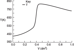
Analysis: From Figure E12-5.1 we see that the temperature increases slowly up to a reactor volume of 0.4 dm³ then suddenly jumps up (ignites) to a temperature of 850 K. Correspondingly, from Figure E12-5.2 the reactant molar flow rate decreases sharply at this point. The reactant is virtually consumed by the time it reaches a reactor volume V - 0.45 dm³; beyond this point, Q_r > Q_g, and the reactor temperature begins to drop. In addition, the selectivity S˜B/C=FB/FC=55/22.5=2.44 ${\tilde{S}}_{B / C} = F_{B} / F_{C} = 55 / 22.5 = 2.44$ remains constant after this point. If a high selectivity is required, then the reactor should be shortened to V = 0.3 dm³, at which point the selectivity is S˜B/C=20/2=10. ${\tilde{S}}_{B / C} = 20 / 2 = 10 .$

12.6.3 Energy Balance for Multiple Reactions in a CSTR

Recall that for the steady-state mole balance in a CSTR with a single reaction [−F_A0X = r_AV,] and that ΔHRx(T)=ΔHoRx+ΔCP(T−TR) $Δ H_{R x} (T) = Δ H_{R x}^{o} + Δ C_{P} (T - T_{R})$ , so that for T₀ = T_i0 Equation (11-27) may be rewritten as

Q ˙ - W ˙ S - F A 0 Σ Θ j C P j (T - T 0) + [Δ H R x (T)] [r A V] = 0 (11-27 A)

$\begin{matrix} \dot{Q} - {\dot{W}}_{S} - F_{A 0} Σ Θ_{j} C_{P_{j}} (T - T_{0}) + [Δ H_{R x} (T)] [r_{A} V] = 0 & \begin{matrix} (11-27 A) \end{matrix} \end{matrix}$

Again, we must account for the “heat generated” by all the reactions in the reactor. For q multiple reactions and m species, the CSTR energy balance becomes

Energy balance for multiple reactions in a CSTR

Q˙−W˙s−FA0Σj=1mΘjCPj(T−T0)+VΣi=1qrijΔHRxij(T)=0(12−39) $\begin{matrix} \dot{Q} - {\dot{W}}_{s} - F_{A0} Σ_{j = 1}^{m} Θ_{j} C_{P_{j}} (T - T_{0}) + V Σ_{i = 1}^{q} r_{i j} Δ H_{Rx i j} (T) = 0 & \begin{matrix} (12 - 39) \end{matrix} \end{matrix}$

Substituting Equation (12-20) for Q˙ $\dot{Q}$ , neglecting the work term, and assuming constant heat capacities and large coolant flow rates m˙c ${\dot{m}}_{c}$ , Equation (12-39) becomes

UA(Ta−T)−FA0Σj=1mCPjΘj(T−T0)+VΣi=1qrijΔHRxij(T)=0(12−40) $\begin{matrix} U A (T_{a} - T) - F_{A0} Σ_{j = 1}^{m} C_{P_{j}} Θ_{j} (T - T_{0}) + V Σ_{i = 1}^{q} r_{i j} Δ H_{Rx i j} (T) = 0 & \begin{matrix} (12 - 40) \end{matrix} \end{matrix}$

For the two parallel reactions described in Example 12-5, the CSTR energy balance is

U A (T a - T) - F A 0 \sum m j = 1 Θ j C P j (T - T 0) + V r 1 A Δ H R x l A (T) + V r 2 A Δ H R x 2 A (T) = 0 (12-41)

$\begin{matrix} U A (T_{a} - T) - F_{A 0} \sum_{j = 1}^{m} Θ_{j} C_{P_{j}} (T - T_{0}) + V r_{1 A} Δ H_{R x l A} (T) + V r_{2 A} Δ H_{R x 2 A} (T) = 0 & \begin{matrix} (12-41) \end{matrix} \end{matrix}$

Major goal

As stated previously, one of the major goals of this text is to have the reader solve problems involving multiple reactions with heat effects (cf. Problems P12-23_C, P12-24_C, P12-25_C, and P12-26_B). That’s exactly what we are doing in the next two examples!

12.6.4 Series Reactions in a CSTR

Example 12-6 Multiple Reactions in a CSTR

The elementary liquid-phase reactions

A→k1B→k2C $A \overset{k_{1}}{\to} B \overset{k_{2}}{\to} C$

take place in a 10-dm³ CSTR. What are the effluent concentrations for a volumetric feed rate of 1000 dm³/min at a concentration of A of 0.3 mol/dm³? The inlet temperature is 283 K.

Additional information

CPA=CPB=CPC=200J/mol⋅Kk1=3.3min−1at 300 K, with E1=9900cal/molk2=4.58min−1at 500 k, with E2=27,000cal/molΔHRx1A=−55,000J/mol A UA=40,000J/min⋅K with Ta=57∘CΔHRx2B=−71,500J/mol B $\begin{array}{l} C_{P_{A}} = C_{P_{B}} = C_{P_{C}} = 200 J/mol \cdot K \\ k_{1} = 3.3 {min}^{- 1} at 300 K, with E_{1} = 9900 cal/mol \\ k_{2} = 4.58 {min}^{- 1} at 500 k, with E_{2} = 27, 000 cal/mol \\ Δ H_{Rx1A} = - 55, 000 J/mol A U A = 40, 000 J/min \cdot {K with T}_{a} = 57^{\circ} C \\ Δ H_{Rx2B} = - 71, 500 J / mol B \end{array}$

Solution

The Algorithm:

0. Number Each Reaction

Reaction (1)Reaction (2)A−→−−−k1BB−→−−−k2C $\begin{matrix} Reaction (1) & A \overset{k_{1}}{\to} B \\ Reaction (2) & B \overset{k_{2}}{\to} C \end{matrix}$

1. Mole Balance on Every Species

Species A: Combined mole balance and rate law for A

V = F A 0 - F A - r A = v 0 [ C A 0 - C A ] - r 1 A = v 0 [ C A 0 - C A ] k 1 C A (E 12-6.1)

$\begin{matrix} V = \frac{F_{A 0} - F_{A}}{- r_{A}} = \frac{v_{0} [C_{A 0} - C_{A}]}{- r_{1 A}} = \frac{v_{0} [C_{A 0} - C_{A}]}{k_{1} C_{A}} & \begin{matrix} (E 12–6.1) \end{matrix} \end{matrix}$

Solving for C_A gives us

C A = C A 0 1 + τ k 1 (E 12-6.2)

$\begin{matrix} C_{A} = \frac{C_{A 0}}{1 + τ k_{1}} & \begin{matrix} (E 12–6.2) \end{matrix} \end{matrix}$

Species B: Combined mole balance and rate law for B

V = 0 - C B v 0 - r B = C B v 0 r B (E 12-6.3)

$\begin{matrix} V = \frac{0 - C_{B} v_{0}}{- r_{B}} = \frac{C_{B} v_{0}}{r_{B}} & \begin{matrix} (E 12–6.3) \end{matrix} \end{matrix}$

2. Rates

The reactions follow elementary rate laws

(a)Lawsr1A=−k1ACA≡−k1CAr2B=−k2BCB≡−k2CB(b)Relative Ratesr1B=−r1Ar2C=−r2B(c)Net RatesrA=r1ArB=r1B+r2B $\begin{matrix} (a) Laws & (b) Relative Rates & (c) Net Rates \\ r_{1 A} = - k_{1A} C_{A} \equiv - k_{1} C_{A} & r_{1 B} = - r_{1 A} & r_{A} = r_{1 A} \\ r_{2 B} = - k_{2 B} C_{B} \equiv - k_{2} C_{B} & r_{2 C} = - r_{2 B} & r_{B} = r_{1 B} + r_{2 B} \end{matrix}$

3. Combine

Substituting for r_1B and r_2B in Equation (E12-6.3) gives

V = C B v 0 k 1 C A - k 2 C B (E 12-6.4)

$\begin{matrix} V = \frac{C_{B} v_{0}}{k_{1} C_{A} - k_{2} C_{B}} & \begin{matrix} (E 12–6.4) \end{matrix} \end{matrix}$

Solving for C_B yields

C B = τ k 1 C A 1 + τ k 2 = τ k 1 C A 0 ( 1 + τ k 1 ) ( 1 + τ k 2 ) (E 12-6.5)

$\begin{matrix} C_{B} = \frac{τ k_{1} C_{A}}{1 + τ k_{2}} = \frac{τ k_{1} C_{A 0}}{(1 + τ k_{1}) (1 + τ k_{2})} & \begin{matrix} (E 12–6.5) \end{matrix} \end{matrix}$

−r1A =k1CA=k1CA01+τk1(E12−6.6) $\begin{matrix} - r_{1 A} = k_{1} C_{A} = \frac{k_{1} C_{A 0}}{1 + τ k_{1}} & (\begin{matrix} E 12 - 6.6 \end{matrix}) \end{matrix}$

−r2B=k2CB=k2τk1CA0(1+τk1)(1+τk2)(E12−6.7) $\begin{matrix} - r_{2 B} = k_{2} C_{B} = \frac{k_{2} τ k_{1} C_{A 0}}{(1 + τ k_{1}) (1 + τ k_{2})} & (\begin{matrix} E 12 - 6.7 \end{matrix}) \end{matrix}$

4. Energy Balances

Applying Equation (12-41) to this system gives

[r 1 A Δ H R x l A + r 2 B Δ H R x 2 B] V - U A (T - T a) - F A 0 C P A (T - T 0) = 0 (E 12-6.8)

$\begin{matrix} [r_{1 A} Δ H_{R x l A} + r_{2 B} Δ H_{R x 2 B}] V - U A (T - T_{a}) - F_{A 0} C_{P_{A}} (T - T_{0}) = 0 & \begin{matrix} (E 12–6.8) \end{matrix} \end{matrix}$

Substituting for F_A0 = υ₀C_A0, r_1A, and r_2B and rearranging, we have

[−ΔHRx1Aτk11+τk1−τk1τk2ΔHRx2B(1+τk1)(1+τk2)]G(T)=CPA(1+K)[T−Tc]R(T)(E12-6.9) $\begin{matrix} \overset{G (T)}{\overset{︷}{[- \frac{Δ H_{R x 1 A} τ k_{1}}{1 + τ k_{1}} - \frac{τ k_{1} τ k_{2} Δ H_{R x 2 B}}{(1 + τ k_{1}) (1 + τ k_{2})}]}} = \overset{R (T)}{\overset{︷}{C_{P_{A}} (1 + K) [T - T_{c}]}} & (E12-6.9) \end{matrix}$

G(T)=[−ΔHRx1Aτk11+τk1−τk1τk2ΔHRx2B(1+τk1)(1+τk2)](E12-6.10) $\begin{matrix} G (T) = [- \frac{Δ H_{R x 1 A} τ k_{1}}{1 + τ k_{1}} - \frac{τ k_{1} τ k_{2} Δ H_{R x 2 B}}{(1 + τ k_{1}) (1 + τ k_{2})}] & (E12-6.10) \end{matrix}$

R(T)=CPA(1+k)[T−Tc](E12-6.11) $\begin{matrix} R (T) = C_{P_{A}} (1 + k) [T - T_{c}] & (E12-6.11) \end{matrix}$

5. Parameter Evaluation

κ = U A F A 0 C P A = 40 , 000 J/min \cdot K ( 0.3 mol/dm 3 ) ( 1000 dm 3 / min ) 200 J/mol \cdot K = 0.667 (E 12-6.12)

$\begin{matrix} κ = \frac{U A}{F_{A 0} C_{P_{A}}} = \frac{40, 000 J/min \cdot K}{(0.3 mol/dm^{3}) (1000 dm^{3} / \min) 200 J/mol \cdot K} = 0.667 & \begin{matrix} (E 12–6.12) \end{matrix} \end{matrix}$

T c = T 0 + κ T a 1 + κ = 2 8 3 + ( 0 . 6 6 6 ) ( 3 3 0 ) 1 + 0 . 6 6 7 = 301.8 K (E 12-6.13)

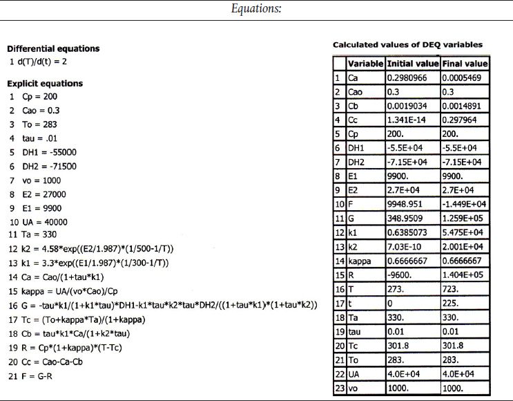
$\begin{matrix} T_{c} = \frac{T_{0} + κ T_{a}}{1 + κ} = \frac{283 + (0.666) (330)}{1 + 0.667} = 301.8 K & \begin{matrix} (E 12–6.13) \end{matrix} \end{matrix}$

We are going to generate G(T) and R(T) by "fooling" Polymath to first generate T as a function of a dummy variable, t. We then use our plotting options to convert T(t) to G(T) and R(T). The Polymath program to plot R(T) and G(T) vs. T is shown in Table E12-6.1, and the resulting graph is shown in Figure E12-6.1 (http://www.umich.edu/~elements/5e/tutorials/Polymath_fooling_tutorial_Example-12-6.pdj).

Incrementing temperature in this manner is an easy way to generate R(T) and G(T) plots.

Table E12-6.1 Polymath: Program and Uutput

Living Example Problem

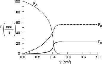
When F = 0, then G(T) = R(T) and the steady states can be found.

Wow! Five (5) multiple steady states!

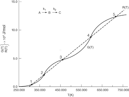
Graph depicts heat-removed and heat-generated curves.

Figure E12-6.1 Heat-removed and heat-generated curves.

Analysis: Wow! We see that five steady states (SS) exist!! The exit concentrations and temperatures listed in Table E12-6.2 were determined from the tabular output of the Polymath program. Steady states 1, 3, and 5 are stable steady states, while 2 and 4 are unstable. The selectivity at steady state 3 is S˜B/C=0.2650.002=132.5 ${\tilde{S}}_{B / C} = \frac{0.265}{0.002} = 132.5$ , while at steady state 5 the selectivity is S˜B/C=0.0050.294=0.017 ${\tilde{S}}_{B / C} = \frac{0.005}{0.294} = 0.017$ and is far too small. Consequently, we either have to operate at steady state 3 or find a different set of operating conditions. What do you think of the value of tau, i.e., τ = 0.01 min? Is it a realistic number? (See P12-1 (h).)

Table E12-6.2 Effluent Concentrations and Temperatures

SS	T(K)	C_A (mol/dm³)	C_B (mol/dm³)	C_C (mol/dm³)
1	310	0285	0.015	0
2	363	0.189	0.111	0.0
3	449	0.033	0.265	0.002
4	558	0.0004	0.163	0.132
5	677	0.001	0.005	0.294

12.6.5 Complex Reactions in a PFR

Example 12-7 Complex Reactions with Heat Effects in a PFR

The following complex gas-phase reactions follow elementary rate laws

(1) 000 A + 2 B \to C 000 - r 1 A = k l A C A C 2 B 0000 Δ H R x l B = - 1 5, 000 c a l / mole 0 B

$(1) A + 2 B \to C - r_{1 A} = k_{l A} C_{A} C_{B}^{2} Δ H_{R x l B} = - 1 5, 0 0 0 c a l / mole B$

(2) 0002 A + 3 C \to D 000 - r 2 C = k 2 C C 2 A C 3 C 0000 Δ H R x 2 A = - 1 0, 000 c a l / mole 0 A

$(2) 2 A + 3 C \to D - r_{2 C} = k_{2 C} C_{A}^{2} C_{C}^{3} Δ H_{R x 2 A} = - 1 0, 0 0 0 c a l / mole A$

and take place in a PFR. The feed is stoichiometric for reaction (1) in A and B with F_A0 = 5 mol/min. The reactor volume is 10 dm³ and the total entering concentration is C_T0 = 0.2 mol/dm³. The entering pressure is 100 atm and the entering temperature is 300 K. The coolant flow rate is 50 mol/min and the entering coolant fluid has a heat capacity of C_P_c0 = 10 cal/mol · K and enters at a temperature of 325 K.

Parameters

0000 K l A = 40 (d m 3 m o 1) 2 / min 00 at 00300 K 00 w i t h 00 E 1 = 8, 000 c a l / m o l 0000 K 2 C = 2 (d m 3 m o 1) 4 / min 00 at 00300 K 00 w i t h 00 E 2 = 12, 000 c a l / m o l C P A = 10 c a l / m o l / K 00 U a = 80 c a 1 m 3 \cdot min \cdot K C P B = 12 c a l / m o l / K 00 T a 0 = 325 K C P C = 14 c a l / m o l / K 00 m . = 50 m o 1 / min C P D = 16 c a l / m o l / K 00 C P C 0 = 10 c a l / m o l / K

$\begin{array}{l} K_{l A} = 40 (\frac{d m^{3}}{m o 1})^{2} / \min at 300 K w i t h E_{1} = 8, 000 c a l / m o l \\ K_{2 C} = 2 (\frac{d m^{3}}{m o 1})^{4} / \min at 300 K w i t h E_{2} = 12, 000 c a l / m o l \\ C_{P_{A}} = 10 c a l / m o l / K U a = 80 \frac{c a 1}{m^{3} \cdot \min \cdot K} \\ C_{P_{B}} = 12 c a l / m o l / K T_{a 0} = 325 K \\ C_{P_{C}} = 14 c a l / m o l / K \dot{m} = 50 m o 1 / \min \\ C_{P_{D}} = 16 c a l / m o l / K C_{P_{C 0}} = 10 c a l / m o l / K \end{array}$

Plot F_A, F_B, F_C, F_D, p, T, and T_a as a function of V for

(a) Co-current heat exchange

(b) Countercurrent heat exchange

(c) Constant T_a

(d) Adiabatic operation

Solution

Gas Phase PFR No Pressure Drop (p = 1)

1. Mole Balances:

(1) d F A d V = r A (2) d F B d V = r B (3) d F C d V = r C (4) d F D d V = r D (F A0 = 50 mol/min) (F B0 = 100 mol/min) V f = 100 dm 3 (E12-7.1) (E12-7.2) (E12-7.3) (E12-7.4)

$\begin{matrix} (1) \frac{d F_{A}}{d V} = r_{A} & (F_{A0} = 5 mol/min) & (E12-7.1) \\ (2) \frac{d F_{B}}{d V} = r_{B} & (F_{B0} = 10 mol/min) & (E12-7.2) \\ (3) \frac{d F_{C}}{d V} = r_{C} & V_{f} = 10 {dm}^{3} & (E12-7.3) \\ (4) \frac{d F_{D}}{d V} = r_{D} & (E12-7.4) \end{matrix}$

Following the Algorithim

2. Rates:

2a. Rate Laws

(5) (6) r 1 A = - k 1 A C A C 2 B r 2 C = - k 2 C C 2 A C 3 C (E12-7.5) (E12-7.6)

$\begin{array}{l} \end{array} \begin{matrix} (5) & r_{1 A} = - k_{1 A} C_{A} C_{B}^{2} & (E12-7.5) \\ (6) & r_{2 C} = - k_{2 C} C_{A}^{2} C_{C}^{3} & (E12-7.6) \end{matrix}$

2b. Relative Rates

(7) (8) (9) (10) r 1 B = 2 r 1 A r 1 C = - r 1 A r 2 A = 2 3 r 2 C = - 2 3 k 2 C C 2 A C 3 C r 2 D = - 1 3 r 2 C = - 1 3 k 2 C C 2 A C 3 C (E12-7.7) (E12-7.8) (E12-7.9) (E12-7.10)

$\begin{matrix} (7) & r_{1 B} = 2 r_{1 A} & (E12-7.7) \\ (8) & r_{1 C} = - r_{1 A} & (E12-7.8) \\ (9) & r_{2 A} = \frac{2}{3} r_{2 C} = - \frac{2}{3} k_{2 C} C_{A}^{2} C_{C}^{3} & (E12-7.9) \\ (10) & r_{2 D} = - \frac{1}{3} r_{2 C} = - \frac{1}{3} k_{2 C} C_{A}^{2} C_{C}^{3} & (E12-7.10) \end{matrix}$

2c. Net Rates of reaction for species A, B, C, and D are

(11)(12)(13)(14)rA=r1A+r2A=−k1ACAC2B−23k2CC2AC3ArB=r1B=−2klACAC2Brc=r1C+r2C=klACAC2B−k2CC2AC3crD = r2D = 13 k2C C2A C3c(E12-7.11)(E12-7.12)(E12-7.13)(E12-7.14) $\begin{matrix} \begin{matrix} (11) & r_{A} = r_{1 A} + r_{2 A} = - k_{1 A} C_{A} C_{B}^{2} - \frac{2}{3} k_{2 C} C_{A}^{2} C_{A}^{3} \\ (12) & r_{B} = r_{1 B} = - 2 k_{l A} C_{A} C_{B}^{2} \\ (13) & r_{c} = r_{1 C} + r_{2 C} = k_{l A} C_{A} C_{B}^{2} - k_{2 C} C_{A}^{2} C_{c}^{3} \\ (14) & r_{D} = r_{2 D} = \frac{1}{3} k_{2 C} C_{A}^{2} C_{c}^{3} \end{matrix} & \begin{matrix} (E12-7.11) \\ (E12-7.12) \\ (E12-7.13) \\ (E12-7.14) \end{matrix} \end{matrix}$

Major goal of CRE

3. Selectivity:

At V = 0, F_D = 0 causing S_C/_D to go to infinity. Therefore, we set S_C/_D = 0 between v = 0 and a very small number, say, v = 0.0001 dm³ to prevent the ODE solver from crashing.

(15) 000 S C/D = if 0 (V>0.0001) 0 then 0 (F C F D) else(0) 000000000 (E12-7.15)

$(15) S_{C/D} = if (V>0.0001) then (\frac{F_{C}}{F_{D}}) else(0) (E12-7.15)$

4. Stoichiometry:

(16) 0000 C A = C T0 (F A F T) P (T 0 T) 000000000000000000000000000000 (E12-7.16) (17) 0000 C B = C T0 (F B F T) P (T 0 T) 00000000000000000000000000000 (E12-7.17)

$\begin{array}{l} (16) C_{A} = C_{T0} (\frac{F_{A}}{F_{T}}) P (\frac{T_{0}}{T}) (E12-7.16) \\ (17) C_{B} = C_{T0} (\frac{F_{B}}{F_{T}}) P (\frac{T_{0}}{T}) (E12-7.17) \end{array}$

(18) 0000 C C = C T0 (F C F T) P (T 0 T) 000000000000000000000000000000 (E12-7.18) (19) 0000 C D = C T0 (F D F T) P (T 0 T) 00000000000000000000000000000 (E12-7.19)

$\begin{array}{l} (18) C_{C} = C_{T0} (\frac{F_{C}}{F_{T}}) P (\frac{T_{0}}{T}) (E12-7.18) \\ (19) C_{D} = C_{T0} (\frac{F_{D}}{F_{T}}) P (\frac{T_{0}}{T}) (E12-7.19) \end{array}$

Neglect pressure drop

(20) 0000 P = 100000000000000000000000000000000000000000000000 (E12-7.20) (21) 0000 F T = F A + F B + F C + F D 00000000000000000000000000000 (E12-7.21)

$\begin{array}{l} (20) P = 1 (E12-7.20) \\ (21) F_{T} = F_{A} + F_{B} + F_{C} + F_{D} (E12-7.21) \end{array}$

5. Parameters:

(22) 0000 K 1 A = 40 exp[E 1 R (1 300 - 1 T)] (dm 3 / mol) 2 / min 0000000000000000000000000 (E12-7.22) (23) 0000 K 2 C = 2 exp[E 2 R (1 300 - 1 T)] (dm 3 / mol) 4 / min 0000000000000000000000000 (E12-7.23)

$\begin{array}{l} (22) K_{1 A} = 40 exp[\frac{E_{1}}{R} (\frac{1}{300} - \frac{1}{T})] ({dm}^{3} / mol)^{2} / min (E12-7.22) \\ (23) K_{2 C} = 2 exp[\frac{E_{2}}{R} (\frac{1}{300} - \frac{1}{T})] ({dm}^{3} / mol)^{4} / min (E12-7.23) \end{array}$

(24) C_A0 = 0.2mol/dm³

(25) R= 1.987cal/mol/K

(26) E₁ = 8,000cal/mol

(27) E₂ = 12,000cal/mol

other parameters are given in the problem statement, i.e., Equations (28) to (34) below.

(28) Cp_A, (29) Cp_B, (30) Cp_c, (31) m˙c ${\dot{m}}_{c}$ , (32) ΔHR∘x1B $Δ H \overset{\circ}{R} x 1 B$ , (33) ΔHR∘x2A $Δ H \overset{\circ}{R} x 2 A$ , (34) Cp₀

6. Energy Balance:

Recalling Equation (12-37)

(35) 000 d T d V = Q g - Q r Σ F j C P j 00000000000000000000000 (E12-7.35)

$(35) \frac{d T}{d V} = \frac{Q_{g} - Q_{r}}{Σ F_{j} C_{P_{j}}} (E12-7.35)$

The denominator of Equation (E12-7.36) is

(36) 000 Σ F j C P j = F A C P A + F B C P B + F C C P C + F D C P D 00000000000000000000000 (E12-7.36)

$(36) Σ F_{j} C_{P_{j}} = F_{A} C_{P_{A}} + F_{B} C_{P_{B}} + F_{C} C_{P_{C}} + F_{D} C_{P_{D}} (E12-7.36)$

The “heat removed” term is

Q r = U a (T - T a)

$Q_{r} = U_{a} (T - T_{a})$

The “heat generated” is

(38) Q g = Σ r i j Δ H Rxij = r 1 B Δ H Rx1B + r 2 A Δ H Rx2 A (E12-7.38)

$(38) Q_{g} = Σ r_{i j} Δ H_{Rxij} = r_{1 B} Δ H_{Rx1B} + r_{2 A} Δ H_{Rx2 A} (E12-7.38)$

(a) Co-current heat exchange

The heat exchange balance for co-current exchange is

(39) 000 d T a d V = U a ( T - T a ) m ˙ c C p CD 00000000000000000000000 (E12-7.39)

$(39) \frac{d T_{a}}{d V} = \frac{U a (T - T_{a})}{{\dot{m}}_{c} C_{p_{CD}}} (E12-7.39)$

Part (a) Co-current flow: Plot and analyze the molar flow rates, and the reactor and coolant temperatures as a function of reactor volume. The Polymath code and output for co-current flow are shown in Table E12-7.1.

Table E12-7.1 Polymath Program and Output for Co-current Exchange

Co-current heat exchange

Living Example Problem

The temperature and molar flow rate profiles are shown in Figure E12-7.1.

Both the graphs are labeled Example 12-7 Co-current Heat Exchange at the top. In graph (a) at left, the horizontal axis representing volume V (cubic decimeter) is marked from 1 to 10 in increments of 1 and the vertical axis representing temperature T in Kelvin is marked from 300 to 900 in increments of 60. A curve representing T subscript a starts from 325 in the vertical axis, remains steady up to 5 cubic decimeter, and then increases gradually until it reaches 506.2 Kelvin. Another curve representing T starts from 300 Kelvin and increases gradually up to 885.7 Kelvin and then the curve decreases up to 524.3 Kelvin. In graph (b) at right, the horizontal axis representing volume V (cubic decimeter) is marked from 0 to 10 in increments of 1 and the vertical axis representing F subscript j (mole per minute) is also marked from 0 to 10 in increments of 1. A curve representing F subscript A starts from 5 moles per minute and remains almost steady up to 4 cubic decimeters. The curve then plunges up to 6 cubic decimeters and then it becomes steady at 0.38 moles per minute. Another curve representing F subscript B starts from 10 moles per minute and decreases gradually up to 4 cubic decimeters. The curve then plunges up to 6 cubic decimeters and then decreases gradually once again up to 0.79 moles per minute. Another curve representing F subscript C starts from 0.5 cubic decimeters and increases gradually up to 4 cubic decimeters. The curve then increases swiftly up to 5.5 cubic decimeters and then it once again increases gradually up to 4.6 moles per minute. The curve F subscript C intersects with the curve F subscript A between 4 and 5 cubic decimeters and intersects with the curve F subscript B close to 5 cubic decimeters.

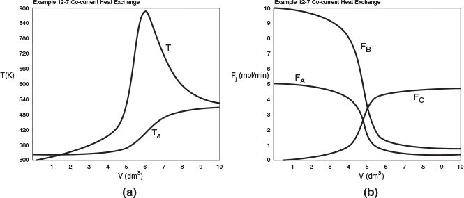
Figure E12-7.1 Profiles for co-current heat exchange; (a) temperature (b) molar flow rates. Note: The molar flow rate F_D is very small and is essentially the same as the bottom axis.

Analysis: Part (a): We also note that the reactor temperature, T, increases when Q_g > Q_r and reaches a maximum, T = 930 K, at approximately V = 5 dm³. After that, Q_r > Q_g the reactor temperature decreases and approaches T_a at the end of the reactor. For co-current heat exchange, the selectivity S˜c/D=4.630.026=178 ${\tilde{S}}_{c / D} = \frac{4.6 3}{0.0 2 6} = 1 7 8$ is really quite good.

Part (b) Countercurrent heat exchange: We will use the same program as part (a), but will change the sign of the heat-exchange balance and guess T_a at V = 0 to be 507 K and see if the value gives us a T_a0 of 325 K at V = V_f.

d T a d V = - U a ( T - T a ) m ˙ c C P Cool

$\frac{d T_{a}}{d V} = - \frac{U a (T - T_{a})}{{\dot{m}}_{c} C_{P_{Cool}}}$

We find our guess of 507 K matches T_a0 = 325 K. Are we lucky or what?!

Table E12-7.2 Polymath Program and Output for Countercurrent Exchange

Countercurrent heat exchange

Living Example Problem

Both the graphs are labeled Example 12-7 Counter current Heat Exchange at the top. In graph (a) at left, the horizontal axis representing volume V (cubic decimeter) is marked from 1 to 10 in increments of 1 and the vertical axis representing temperature T in Kelvin is marked from 300 to 2000 in increments of 90 up to 1100 and then 2000 is marked. A curve representing T subscript a starts from 507 Kelvin, increases up to 536 Kelvin, and then it starts decreasing up to 5 cubic decimeters and becomes steady at 325.4 Kelvin. Another curve representing T starts from 300 Kelvin and increases gradually up to 1101 Kelvin and then the curve decreases up to 327 Kelvin. In graph (b) at right, the horizontal axis representing volume V (cubic decimeter) is marked from 0 to 10 in increments of 1 and the vertical axis representing F subscript j (mole per minute) is also marked from 0 to 10 in increments of 1. A curve representing F subscript A starts from 5 moles per minute and remains almost steady up to 1 cubic decimeter. The curve then plunges up to 2 cubic decimeters and then it becomes steady at 0.38 moles per minute. Another curve representing F subscript B starts from 10 moles per minute and decreases gradually up to 1 cubic decimeter. The curve then plunges up to 2.5 cubic decimeters and then becomes steady at 0.78 moles per minute. Another curve representing F subscript C starts from 0.5 cubic decimeters and increases swiftly up to 2 cubic decimeters. The curve then becomes steady at 4.6 moles per minute. The curve F subscript C intersects with the curve F subscript A between 1 and 2 cubic decimeters and intersects with the curve F subscript B at 2 cubic decimeters. Another curve representing F subscript D is drawn over the horizontal axis.

Figure E12-7.2 Profiles for countercurrent heat exchange; (a) temperature (b) molar flow rates.

Analysis: Part (b): For countercurrent exchange, the coolant temperature reaches a maximum at V = 1.3 dm³ while the reactor temperature reaches a maximum at V = 2.7 dm³. The reactor with a countercurrent exchanger reaches a maximum reactor temperature of 1100 K, which is greater than that for the co-current exchanger, (i.e., 930 K). Consequently, if there is a concern about additional side reactions occurring at this maximum temperature of 1100 K, one should use a co-current exchanger or if possible use a large coolant flow rate to maintain constant Ta in the exchanger. In Figure 12-7.2 (a) we see that the reactor temperature approaches the coolant entrance temperature at the end of the reactor. The selectivity for the coun-tercurrent systems S¯¯C/D=175, ${\bar{S}}_{C/D} = 175,$ is slightly lower than that for the co-current exchange.

Part (c) Constant T_a: To solve the case of constant heating-fluid temperature, we simply multiply the right-hand side of the heat-exchanger balance by zero, i.e.,

d T a d V = - U a ( T - T a ) m . c C P * 0

$\frac{d T_{a}}{d V} = - \frac{U a (T - T_{a})}{{\dot{m}}_{c} C_{P}} * 0$

and use Equations (E12-7.1) through (E12-7.39).

Table E12-7.3 Polymath Program and Output for Constant T_a

Constant T_a

Both the graphs are labeled Example 12-7 Constant T subscript a at the top. In graph (a) at left, the horizontal axis representing volume V (cubic decimeter) is marked from 1 to 10 in increments of 1 and the vertical axis representing temperature T in Kelvin is marked from 300 to 900 in increments of 60. A horizontal line representing T subscript a is drawn at 325 Kelvin. Another curve representing T starts from 300 Kelvin and increases gradually up to 836.9 Kelvin and then the curve decreases up to 345.6 Kelvin. In graph (b) at right, the horizontal axis representing volume V (cubic decimeter) is marked from 0 to 10 in increments of 1 and the vertical axis representing F subscript j (mole per minute) is also marked from 0 to 10 in increments of 1. A curve representing F subscript A starts from 5 moles per minute and decreases very gradually up to 4 cubic decimeters. The curve then plunges up to 5.5 cubic decimeters and then it becomes steady at 0.5 moles per minute. Another curve representing F subscript B starts from 10 moles per minute and decreases gradually up to 4 cubic decimeters. The curve then plunges up to 5.5 cubic decimeters and then becomes steady at 1 mole per minute. Another curve representing F subscript C starts from 1 cubic decimeter and increases gradually up to 5.5 cubic decimeters. The curve then becomes steady at 4.4 moles per minute. The curve F subscript C intersects with the curve F subscript A between 4 and 5 cubic decimeters and intersects with the curve F subscript B close to 5 cubic decimeters. Another curve representing F subscript D is drawn over the horizontal axis.

Figure E12-7.3 Profiles for constant T_a; (a) temperature (b) molar flow rates.

Analysis: Part (c): For constant T_a, the maximum reactor temperature, 870K, is less than either co-current or countercurrent exchange while the selectivity, S¯¯C/D=252.9 ${\bar{S}}_{C/D} = 252.9$ is greater than either co-current or countercurrent exchange. Consequently, one should investigate how to achieve suff iciently high mass flow of the coolant in order to maintain constant Ta.

Part (d) Adiabatic: To solve for the adiabatic case, we simply multiply the overall heat transfer coefficient by zero.

Ua=80*0

Table E12-7.4 Polymath Program and Output for Adiabatic Operation

Living Example Problem

Adiabatic operation

Both the graphs are labeled Example 12-7 Adiabatic at the top. In graph (a) at left, the horizontal axis representing volume V (cubic decimeter) is marked from 0 to 10 in increments of 1 and the vertical axis representing temperature T in Kelvin is marked from 0 to 2000 in increments of 200. A curve representing T starts from 300 Kelvin and increases very gradually up to 4 cubic decimeters. The curve then increases swiftly up to 5 cubic decimeters and then it again increases gradually up to 1548 Kelvin. In graph (b) at right, the horizontal axis representing volume V (cubic decimeter) is marked from 0 to 10 in increments of 1 and the vertical axis representing F subscript j (mole per minute) is also marked from 0 to 10 in increments of 1. A curve representing F subscript A starts from 5 moles per minute and decreases very gradually up to 4 cubic decimeters. The curve then plunges up to 5.5 cubic decimeters and then it becomes almost steady at 0.18 moles per minute. Another curve representing F subscript B starts from 10 moles per minute and decreases gradually up to 4 cubic decimeters. The curve then plunges up to 5.5 cubic decimeters and then it decreases very gradually up to 0.4 moles per minute. Another curve representing F subscript C starts from 1 cubic decimeter and increases gradually up to 5.5 cubic decimeters. The curve then becomes almost steady at 4.7 moles per minute. The curve F subscript C intersects with the curve F subscript A between 4 and 5 cubic decimeters and intersects with the curve F subscript B close to 5 cubic decimeters. Another curve representing F subscript D is drawn over the horizontal axis.

Figure E12-7.4 Profiles for adiabatic operation

Analysis: Part (d): For the adiabatic case, the maximum temperature, which is the exit temperature, is higher than the other three exchange systems, and the selectivity is the lowest. At this high temperature, the occurrence of unwanted side reactions certainly is a concern.

Overall Analysis Parts (a) to (d): Suppose the maximum temperature in each of these cases is outside the safety limit of 750 K for this system. Problem P12-2_A (i) asks how you can keep the maximum temperature below 750 K.

12.7 Radial and Axial Variations in a Tubular Reactor

COMSOL application

In the previous sections, we have assumed that there were no radial variations in velocity, concentration, temperature, or reaction rate in the tubular and packed-bed reactors. As a result, the axial profiles could be determined using an ordinary differential equation (ODE) solver. In this section, we will consider the case where we have both axial and radial variations in the system variables, in which case we will require a partial differential (PDE) solver. A PDE solver such as COMSOL will allow us to solve tubular reactor problems for both the axial and radial profiles, as shown in the Radial Effects COMSOL Web module on the CRE Web site (http://www.umich.edu/~elements/5e/web_mod/radialeffects/index.htm.⁷ In addition, a number of COMSOL examples associated with and developed for this book are available from the COMSOL Web site (www.comsol.com/ecre).

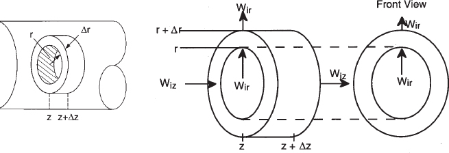
We are going to carry out differential mole and energy balances on the differential cylindrical annulus shown in Figure 12-15.

Schematic shows the three views of a cylindrical shell.

Figure 12-15 Cylindrical shell of thickness Δr, length Δz, and volume 2πrΔrΔz.

⁷ An introductory webinar on COMSOL can be found on the AIChE webinar Web site: http://www.aiche.org/resources/chemeondemand/webinars/modeling-non-ideal-reactors-and-mixers.

12.7.1 Molar Flux

In order to derive the governing equations, we need to define a couple of terms. The first is the molar flux of species i, W_i (mol/m² • s). The molar flux has two components, the radial component, W_ir, and the axial component, W_iz. The molar flow rates are just the product of the molar fluxes and the cross-sectional areas normal to their direction of flow A_cz. For example, for species i flowing in the axial (i.e., z) direction

F_iz = W_iz A_cz

where W_iz is the molar flux in the axial direction (mol/m²/s), and A_cz (m²) is the cross-sectional area of the tubular reactor.

In PDF Chapter 14 on the Web site (http://www.umich.edu/~elements/5e/14chap/Fogler_Web_Ch14.pdf we discuss the molar fluxes in some detail, but for now let’s just say they consist of a diffusional component, -D_e(∂C_i/∂z), and a convective-flow component, U_zC_i, so that the flux in the axial direction is

W i z = - D e \partial C i \partial z + U Z C i 00000000000000000 (12-42)

$W_{i z} = - D_{e} \frac{\partial C_{i}}{\partial z} + U_{Z} C_{i} (12-42)$

where D_e is the effective diffusivity (or dispersion coefficient) (m²/s), and U_z is the axial molar average velocity (m/s). Similarly, the flux in the radial direction, r, is

W i r = - D e \partial C i \partial r + U r C i 00000000000000000 (12-43)

$W_{i r} = - D_{e} \frac{\partial C_{i}}{\partial r} + U_{r} C_{i} (12-43)$

Radial direction

where U_r (m/s) is the average velocity in the radial direction. For now, we will neglect the velocity in the radial direction, i.e., U_r = 0. A mole balance on species A (i.e., i = A) in a cylindrical system volume of length Δz and thickness Δr as shown in Figure 12-15 gives

Mole Balances on Species A

(M oles 0 of 0 A in 0 at 0 r) 0 = 0 W Ar \cdot (C ross- sectional 0 area normal 0 to 0 radial 0 flux) = W Ar \cdot 2 π r Δ z (M oles 0 of 0 A in 0 at 0 z) 0 = 0 W A z \cdot (C ross- sectional 0 area normal 0 to 0 axial 0 flux) = W Az \cdot 2 π r Δ r (M oles 0 of 0 A in 0 at 0 r) - (M oles 0 of 0 A out 0 at 0 ( r + Δ r )) + (M oles 0 of 0 A in 0 at 0 z) - (M oles 0 of 0 A out 0 at 0 ( z + Δ z )) + (M oles 0 of 0 A formed) = (M oles 0 of 0 A accumulated)

$\begin{matrix} (\frac{M oles of A}{in at r}) = W_{Ar} \cdot (\frac{C ross- sectional area}{normal to radial flux}) = W_{Ar} \cdot 2 π r Δ z \\ (\frac{M oles of A}{in at z}) = W_{A z} \cdot (\frac{C ross- sectional area}{normal to axial flux}) = W_{Az} \cdot 2 π r Δ r \\ (\frac{M oles of A}{in at r}) - (\frac{M oles of A}{out at (r + Δ r)}) + (\frac{M oles of A}{in at z}) - (\frac{M oles of A}{out at (z + Δ z)}) \\ + (\frac{M oles of A}{formed}) = (\frac{M oles of A}{accumulated}) \end{matrix}$

W A r 2 π r Δ z | r - W A r A π r Δ z | r + Δ r + W A z 2 π r Δ r | Z - W A z 2 π r Δ r | z + Δ z + r A 2 π r Δ r Δ z = \partial C A ( 2 π r Δ r Δ z ) \partial t

$\begin{matrix} W_{A r} 2 π r Δ z |_{r^{-}} W_{A r} A π r Δ z |_{r + Δ r} + W_{A z} 2 π r Δ r |_{Z^{-}} W_{A z} 2 π r Δ r |_{z + Δ z} \\ + r_{A} 2 π r Δ r Δ z = \frac{\partial C_{A} (2 π r Δ r Δ z)}{\partial t} \end{matrix}$

Dividing by 2πrΔrΔz and taking the limit as Δr and Δz → 0

- 1 r \partial ( r W A r ) \partial r - \partial W A z \partial z + r A = \partial C A \partial t

$- \frac{1}{r} \frac{\partial (r W_{A r})}{\partial r} - \frac{\partial W_{A z}}{\partial z} + r_{A} = \frac{\partial C_{A}}{\partial t}$

Similarly, for any species i and steady-state conditions

−1r∂(rWir)∂r−∂Wiz∂z+ri=0(12-44) $\begin{matrix} - \frac{1}{r} \frac{\partial (r W_{i r})}{\partial r} - \frac{\partial W_{i z}}{\partial z} + r_{i} = 0 & (12 -44) \end{matrix}$

Using Equations (12-42) and (12-43) to substitute for W_iz and W_ir in Equation (12-44) and then setting the radial velocity to zero, U_r = 0, we obtain

- 1 r \partial \partial r [(- D e \partial C i \partial r r)] (- \partial \partial z [- D e \partial C i \partial z + U z C i]) + r i 0 = 00

$- \frac{1}{r} \frac{\partial}{\partial r} [(- D_{e} \frac{\partial C_{i}}{\partial r} r)] (- \frac{\partial}{\partial z} [- D_{e} \frac{\partial C_{i}}{\partial z} + U_{z} C_{i}]) + r_{i} = 0$

For steady-state conditions and assuming U_z does not vary in the axial direction

De∂2Ci∂r2+Der∂Ci∂r+De∂2Ci∂z2−UZ∂Ci∂z+ri=0(12-45) $\begin{matrix} D_{e} \frac{\partial^{2} C_{i}}{\partial r^{2}} + \frac{D_{e}}{r} \frac{\partial C_{i}}{\partial r} + D_{e} \frac{\partial^{2} C_{i}}{\partial z^{2}} - U_{Z} \frac{\partial C_{i}}{\partial z} + r_{i} = 0 & (12 -45) \end{matrix}$

This equation will also be discussed further in PDF Chapter 17 on the Web site.

12.7.2 Energy Flux

When we applied the first law of thermodynamics to a reactor to relate either temperature and conversion or molar flow rates and concentration, we arrived at Equation (11-10). Neglecting the work term we have for steady-state conditions

ConductionQ˙+Σi=1nConvectionFi0Hi0−Σi=1FiHi=0(12-46) $\begin{matrix} \underset{\overset{︷}{\dot{Q}}}{Conduction}_{+ Σ_{i = 1}^{n}}^{} & \underset{\overset{︷}{F_{i 0 H_{i 0} - \underset{i = 1}{Σ} F_{i} H_{i}}}}{Convection}_{= 0}^{} & \begin{matrix} (12-46) \end{matrix} \end{matrix}$

In terms of the molar fluxes and the cross-sectional area, and (q = Q/A_c )

A_c[q + (ΣW_i0H_i0 - ΣW_iH_i)] = 0 (12-47)

The q term is the heat added to the system and almost always includes a conduction component of some form. We now define an energy flux vector, e, (J/m² · s), to include both the conduction and convection of energy.

e = energy flux J/s·m²

e = Conduction + Convection

e=q+ΣWiHi(12-48) $\begin{matrix} e = q + Σ W_{i} H_{i} & (12-48) \end{matrix}$

where the conduction term q (kJ/m² · s) is given by Fourier’s law. For axial and radial conduction, Fourier’s laws are

q Z 0 = - k e \partial T \partial z 0000 and 0000 q r 0 = - k e \partial T \partial r

$q_{Z} = - k_{e} \frac{\partial T}{\partial z} and q_{r} = - k_{e} \frac{\partial T}{\partial r}$

where k_e is the thermal conductivity (J/m·s·K). The energy transfer (flow) is the flux vector times the cross-sectional area, A_c, normal to the energy flux

Energy flow = e · A_c

..................Content has been hidden....................

You can't read the all page of ebook, please click here login for view all page.

Table of Contents for 12.5.2 Heat-GeneratedTerm,G(T)

Create new playlist

Sign In

Sign Up

12.5.2 Heat-Generated Term, G(T)

12.5.3 Ignition-Extinction Curve

12.6 Nonisothermal Multiple Chemical Reactions

12.6.1 Energy Balance for Multiple Reactions in Plug-Flow Reactors

12.6.2 Parallel Reactions in a PFR

12.6.3 Energy Balance for Multiple Reactions in a CSTR

12.6.4 Series Reactions in a CSTR

12.6.5 Complex Reactions in a PFR

12.7 Radial and Axial Variations in a Tubular Reactor

12.7.1 Molar Flux

12.7.2 Energy Flux

Table of Contents for
12.5.2 Heat-GeneratedTerm,G(T)