1. Mole Balances
The first step to knowledge is to know that we are ignorant.
—Socrates (470-399 B.C.)
How is a chemical engineer different from other engineers?
The Wide Wild World of Chemical Reaction Engineering
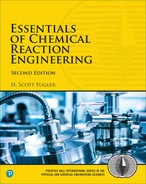
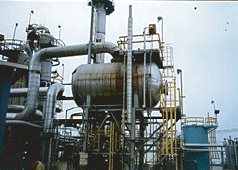
Chemical kinetics is the study of chemical reaction rates and reaction mechanisms. The study of chemical reaction engineering (CRE) combines the study of chemical kinetics with the reactors in which the reactions occur. Chemical kinetics and reactor design are at the heart of producing almost all industrial chemicals, such as the manufacture of phthalic anhydride shown in Figure 1-1. It is primarily a knowledge of chemical kinetics and reactor design that distinguishes the chemical engineer from other engineers. The selection of a reaction system that operates in the safest and most efficient manner can be the key to the economic success or failure of a chemical plant. For example, if a reaction system produces a large amount of undesirable product, subsequent purification and separation of the desired product could make the entire process economically unfeasible.
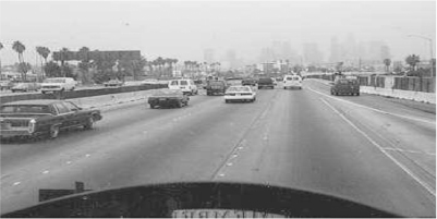
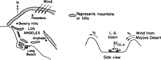
The chemical reaction engineering (CRE) principles learned here can also be applied in many areas, such as waste treatment, microelectronics, nanoparticles, and living systems, in addition to the more traditional areas of the manufacture of chemicals and pharmaceuticals. Some of the examples that illustrate the wide application of CRE principles in this book are shown in Figure 1-2. These examples include modeling smog in the Los Angeles (L.A.) basin (Chapter 1), the digestive system of a hippopotamus (Chapter 2 on the CRE Web site, www.umich.edu/~elements/5e/index.html), and molecular CRE (Chapter 3). Also shown are the manufacture of ethylene glycol (antifreeze), where three of the most common types of industrial reactors are used (Chapters 5 and 6), and the use of wetlands to degrade toxic chemicals (Chapter 7 on the CRE Web site). Other examples shown are the solid-liquid kinetics of acid-rock interactions to improve oil recovery (Chapter 7); pharmacokinetics of cobra bites (Chapter 8 Web Module); free-radical scavengers used in the design of motor oils (Chapter 9); enzyme kinetics (Chapter 9) and drug delivery pharmacokinetics (Chapter 9 on the CRE Web site); heat effects, runaway reactions, and plant safety (Chapters 11 through 13); and increasing the octane number of gasoline and the manufacture of computer chips (Chapter 10).

1.1 The Rate of Reaction, –rA
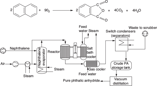
The rate of reaction tells us how fast a number of moles of one chemical species are being consumed to form another chemical species. The term chemical species refers to any chemical component or element with a given identity. The identity of a chemical species is determined by the kind, number, and configuration ofthat species’ atoms. For example, the species para-xylene is made up of a fixed number of specific atoms in a definite molecular arrangement or configuration. The structure shown illustrates the kind, number, and configuration of atoms on a molecular level. Even though two chemical compounds have exactly the same kind and number of atoms of each element, they could still be different species because of different configurations. For example, 2-butene has four carbon atoms and eight hydrogen atoms; however, the atoms in this compound can form two different arrangements.

Identify
– Kind
– Number
– Configuration
As a consequence of the different configurations, these two isomers display different chemical and physical properties. Therefore, we consider them as two different species, even though each has the same number of atoms of each element.
When has a chemical reaction taken place?
We say that a chemical reaction has taken place when a detectable number of molecules of one or more species have lost their identity and assumed a new form by a change in the kind or number of atoms in the compound and/or by a change in structure or configuration of these atoms. In this classical approach to chemical change, it is assumed that the total mass is neither created nor destroyed when a chemical reaction occurs. The mass referred to is the total collective mass of all the different species in the system. However, when considering the individual species involved in a particular reaction, we do speak of the rate of disappearance of mass of a particular species. The rate of disappearance of a species, say species A, is the number of A molecules that lose their chemical identity per unit time per unit volume through the breaking and subsequent re-forming of chemical bonds during the course of the reaction. In order for a particular species to “appear” in the system, some prescribed fraction of another species must lose its chemical identity.
Definition of Rate of Reaction
There are three basic ways a species may lose its chemical identity: decomposition, combination, and isomerization. In decomposition, the molecule loses its identity by being broken down into smaller molecules, atoms, or atom fragments. For example, if benzene and propylene are formed from a cumene molecule,

the cumene molecule has lost its identity (i.e., disappeared) by breaking its bonds to form these molecules. A second way that a molecule may lose its chemical identity is through combination with another molecule or atom. In the above reaction, the propylene molecule would lose its chemical identity if the reaction were carried out in the reverse direction, so that it combined with benzene to form cumene. The third way a species may lose its chemical identity is through isomerization, such as the reaction

A species can lose its identity by
• Decomposition
• Combination
• Isomerization
Here, although the molecule neither adds other molecules to itself nor breaks into smaller molecules, it still loses its identity through a change in configuration.
To summarize this point, we say that a given number of molecules (i.e., moles) of a particular chemical species have reacted or disappeared when the molecules have lost their chemical identity.
The rate at which a given chemical reaction proceeds can be expressed in several ways. To illustrate, consider the reaction of chlorobenzene with chloral to produce the banned insecticide DDT (dichlorodiphenyl-trichloroethane) in the presence of fuming sulfuric acid.
CCl3CHO + 2C6H5Cl → (C6H4Cl)2CHCC13 + H2O
Letting the symbol A represent chloral, B be chlorobenzene, C be DDT, and D be H2O, we obtain
A + 2B → C + D
The numerical value of the rate of disappearance of reactant A, −rA, is a positive number.
What is −rA?
The rate of reaction, −rA, is the number of moles of A (e.g., chloral) reacting (disappearing) per unit time per unit volume (mol/dm3·s).
Example 1-1 Rates of Disappearance and Formation
Chloral is being consumed at a rate of 10 moles per second per m3 when reacting with chlorobenzene to form DDT and water in the reaction described above. In symbol form, the reaction is written as
A + 2B → C + D
Write the rates of disappearance and formation (i.e., generation) for each species in this reaction.
Solution
(a) Chloral[A]: |
The rate of reaction of chloral [A] (—rA) is given as 10mol/m3·s Rate of disappearance of A = –rA = 10 mol/m3·s Rate of formation of A = rA = –10 mol/m3·s |
(b) Chlorobenzene[B]: |
For every mole of chloral that disappears, two moles of chlorobenzene [B] also disappear. Rate of disappearance of B = –rB = 20 mol/m3·s Rate of formation of B = rB = –20 mol/m3·s |
(c) DDT[C]: |
For every mole of chloral that disappears, two moles of DDT[C] appears. Rate of formation of C = rC = 10 mol/m3·s Rate of disappearance of C = –rC = –10 mol/m3·s |
(d) Water[D]: |
Same relationship to chloral as the relationship to DDT Rate of formation of D = rD = 10 mol/m3·s Rate of disappearance of D = –rD = –10 mol/m3·s |
Analysis: The purpose of this example is to better understand the convention for the rate of reaction. The symbol rj is the rate of formation (generation) of species j. If species j is a reactant, the numerical value of rj will be a negative number. If species j is a product, then rj will be a positive number. The rate of reaction, −rA, is the rate of disappearance of reactant A and must be a positive number. A mnemonic relationship to help remember how to obtain relative rates of reaction of A to B, etc., is given by Equation (3-1) on page 73.

A + 2B→C + D
The convention
−rA = 10 mol A/m3·s
rA = -10 mol A/m3·s
−r = 20 mol B/m3·s
rB = –20 mol B/m3·s
rC = 10 mol C/m3·s
In Chapter 3, we will delineate the prescribed relationship between the rate of formation of one species, r> (e.g., DDT [C]), and the rate of disappearance of another species, - η (e.g., chlorobenzene [B]), in a chemical reaction.
Heterogeneous reactions involve more than one phase. In heterogeneous reaction systems, the rate of reaction is usually expressed in measures other than volume, such as reaction surface area or catalyst weight. For a gas-solid catalytic reaction, the gas molecules must interact with the solid catalyst surface for the reaction to take place, as described in Chapter 10.
The dimensions of this heterogeneous reaction rate, (prime), are the number of moles of A reacting per unit time per unit mass of catalyst (mol/sݑg catalyst).
What is ?
Most of the introductory discussions on chemical reaction engineering in this book focus on homogeneous systems, in which case we simply say that η is the rate of formation of species j per unit volume. It is the number of moles of species j generated per unit volume per unit time.
Definition of rj
We can say four things about the reaction rate rj. The reaction rate law for rj is
The rate law does not depend on the type of reactor used!!
• The rate of formation of species; (mole/time/volume)
• An algebraic equation
• Independent of the type of reactor (e.g., batch or continuous flow) in which the reaction is carried out
• Solely a function of the properties of the reacting materials and reaction conditions (e.g., species concentration, temperature, pressure, or type of catalyst, if any) at a point in the system
What is −rA a function of?
However, because the properties and reaction conditions of the reacting materials may vary with position in a chemical reactor, rj can in turn be a function of position and can vary from point to point in the system.
The chemical reaction rate law is essentially an algebraic equation involving concentration, not a differential equation.1 For example, the algebraic form of the rate law for −rA for the reaction
A → products
may be a linear function of concentration,
or it may be some other algebraic function of concentration, such as Equation 3-6 shown in Chapter 3
1 For further elaboration on this point, see Chem. Eng Sei., 25, 337 (1970); B. L. Crynes and H. S. Fogler, eds., AIChE Modular Instruction Series E: Kinetics, 1,1 (New York: AIChE, 1981); and R. L. Kabel, “Rates,” Chem. Eng. Commun., 9, 15 (1981).
or
The rate law is an algebraic equation.
For a given reaction, the particular concentration dependence that the rate law follows (i.e., −rA = kCA or or ...) must be determined from expérimenta! observation. Equation (1-2) states that the rate of disappearance of A is equal to a rate constant k (which is a function of temperature) times the square The convention of the concentration of A. As noted earlier, by convention, rA is the rate of formation of A; consequently, −rA is the rate of disappearance of A. Throughout this book, the phrase rate of generation means exactly the same as the phrase rate of formation, and these phrases are used interchangeably.
The convention
1.2 The General Mole Balance Equation
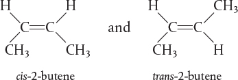
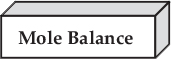
To perform a mole balance on any system, the system boundaries must first be specified. The volume enclosed by these boundaries is referred to as the system volume. We shall perform a mole balance on species j in a system volume, where species j represents the particular chemical species of interest, such as water or NaOH (Figure 1-3).
A mole balance on species j at any instant in time, t, yields the following equation:
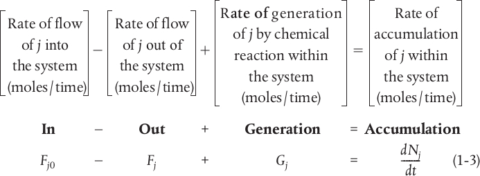
In this equation, Nj represents the number of moles of species j in the system at time t. If all the system variables (e.g., temperature, catalytic activity, and concentration of the chemical species) are spatially uniform throughout the system volume, the rate of generation of species j, Gj, is just the product of the reaction volume, V, and the rate of formation of species j, rj.
Now suppose that the rate of formation of species j for the reaction varies with position in the system volume. That is, it has a value rj1 at location 1, which is surrounded by a small volume, ΔV1, within which the rate is uniform; similarly, the reaction rate has a value rj2 at location 2 and an associated volume, ΔV2, and so on (Figure 1-4).

The rate of generation, ΔGj1, in terms of rj1 and subvolume ΔV1, is
ΔGj1 = rj1 ΔV1
Similar expressions can be written for ΔGj2 and the other system subvolumes, ΔVi. The total rate of generation within the system volume is the sum of all the rates of generation in each of the subvolumes. If the total system volume is divided into M subvolumes, the total rate of generation is
By taking the appropriate limits (i.e., let M → ∞ and ΔV → 0 ) and making use of the definition of an integral, we can rewrite the foregoing equation in the form
From this equation, we see that rj will be an indirect function of position, since the properties of the reacting materials and reaction conditions (e.g., concentration, temperature) can have different values at different locations in the reactor volume.
We now replace Gj in Equation (1-3), i.e.,
by its integral form to yield a form of the general mole balance equation for any chemical species j that is entering, leaving, reacting, and/or accumulating within any system volume V.
This is a basic equation for chemical reaction engineering.
From this general mole balance equation, we can develop the design equations for the various types of industrial reactors: batch, semibatch, and continuous-flow Upon evaluation of these equations, we can determine the time (batch) or reactor volume (continuous-flow) necessary to convert a specified amount of the reac-tants into products.
1.3 Batch Reactors (BRs)
A batch reactor is used for small-scale operation, for testing new processes that have not been fully developed, for the manufacture of expensive products, and for processes that are difficult to convert to continuous operations. The reactor can be charged (i.e., filled) through the holes at the top (see Figure l-5(a)). The batch reactor has the advantage of high conversions that can be obtained by leaving the reactant in the reactor for long periods of time, but it also has the disadvantages of high labor costs per batch, the variability of products from batch to batch, and the difficulty of large-scale production (see Industrial Reactor Photos in Professional Reference Shelf [PRS] on theCRE Web sites, www.umich.edu/~elements/5e/index.html). Also see http://encyclopedia.che.engin.umich.edu/Pages/Reactors/menu.html.
When is a batch reactor used?


Figure 1-5(a) Simple batch homogeneous batch reactor (BR). [Excerpted by special permission from Chem. Eng., 63(10), 211 (Oct. 1956). Copyright 1956 by McGraw-Hill, Inc., New York, NY 10020.]
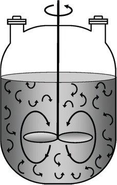
Figure 1-5(b) Batch reactor mixing patterns. Further descriptions and photos of the batch reactors can be found in both the Visual Encyclopedia of Equipment and in the Professional Reference Shelf on the CRE Web site.
Also see http://encyclopedia.che.engin.umich.edu/Pages/Reactors/Batch/Batch.html.
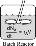
A batch reactor has neither inflow nor outflow of reactants or products while the reaction is being carried out: Fj0 = Fj = 0. The resulting general mole balance on species j is
If the reaction mixture is perfectly mixed (Figure l-5(b)) so that there is no variation in the rate of reaction throughout the reactor volume, we can take η out of the integral, integrate, and write the mole balance in the form
Perfect mixing
Let’s consider the isomerization of species A in a batch reactor
As the reaction proceeds, the number of moles of A decreases and the number of moles of B increases, as shown in Figure 1-6.

We might ask what time, t1, is necessary to reduce the initial number of moles from NA0 to a final desired number NA1. Applying Equation (1-5) to the isomerization
rearranging,
and integrating with limits that at t = 0, then NA = NA0, and at t = t1, then NA = NA1, we obtain
This equation is the integral form of the mole balance on a batch reactor. It gives the time, t1, necessary to reduce the number of moles from NA0 to NA1 and also to form NB1 moles of B.
1.4 Continuous-Flow Reactors
Continuous-flow reactors are almost always operated at steady state. We will consider three types: the continuous-stined tank reactor (CSTR), the plug-flow reactor (PFR), and the packed-beâ reactor (PBR). Detailed physical descriptions of these reactors can be found in both the Professional Reference Shelf (PRS) for Chapter 1 and in the Visual Encyclopedia of Equipment, http://encyclopedia.che.engin.umkh.edu/Pages/Reactors/CSTR/CSTR.html, and on the CRE Web site.
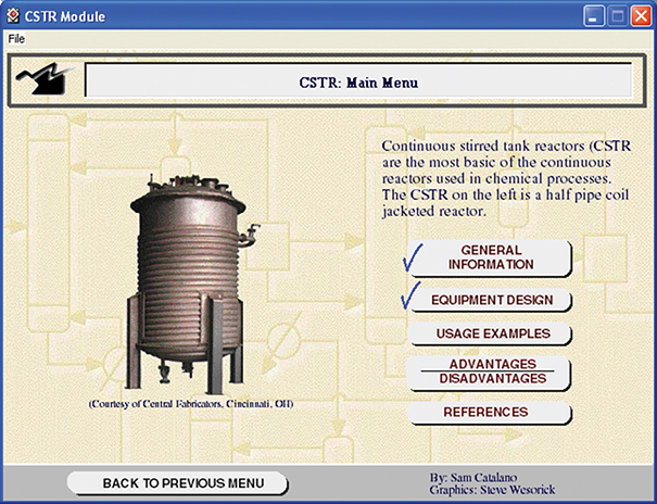
1.4.1 Continuous-Stirred Tank Reactor (CSTR)
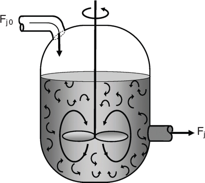
A type of reactor commonly used in industrial processing is the stirred tank operated continuously (Figure 1-7). It is referred to as the continuous-stined tankreactor (CSTR) or vat, or backmix reactor, and is primarily used for
What is a CSTR used for?

Also see http://encyclopeiJia.che.engin.umich.eiJu/Pages/Reactors/CSTR/CSTR.html.
liquid-phase reactions. It is normally operated at steady state and is assumed to be perfectly mixed; consequently there is no time dependence or position dependence of the temperature, concentration, or reaction rate inside the CSTR. That is, every variable is the same at every point inside the reactor. Because the temperature and concentration are identical everywhere within the reaction vessel, they are the same at the exit point as they are elsewhere in the tank. Thus, the temperature and concentration in the exit stream are modeled as being the same as those inside the reactor. In systems where mixing is highly nonideal, the well-mixed model is inadequate, and we must resort to other modeling techniques, such as residence time distributions, to obtain meaningful results. This topic of nonideal mixing is discussed on the Web site in PDF Chapters 16, 17, and 18 on nonideal reactors.
When the general mole balance equation
is applied to a CSTR operated at steady state (i.e., conditions do not change with time),
in which there are no spatial variations in the rate of reaction (i.e., perfect mixing),
The ideal CSTR is assumed to be perfectly mixed.
it takes the familiar form known as the design equation for a CSTR

The CSTR design equation gives the reactor volume V necessary to reduce the entering molar flow rate of species j from Fj0 to the exit molar flow rate Fj, when species; is disappearing at a rate −rj. We note that the CSTR is modeled such that the conditions in the exit stream (e.g., concentration and temperature) are identical to those in the tank. The molar flow rate Fj is just the product of the concentration of species j and the volumetric flow rate υ
Similarly, for the entrance molar flow rate we have Fj0 = Cj0 · υ0. Consequently, we can substitute for Fj0 and Fj into Equation (1-7) to write a balance on species A as
The ideal CSTR mole balance equation is an algebraic equation, not a differential equation.
1.4.2 Tubular Reactor
When is a tubular reactor most often used?
In addition to the CSTR and batch reactors, another type of reactor commonly used in industry is the tubular reactor. It consists of a cylindrical pipe and is normally operated at steady state, as is the CSTR. Tubular reactors are used most often for gas-phase reactions. A schematic and a photograph of industrial tubular reactors are shown in Figure 1-8.

Figure 1-8(a) Tubular reactor schematic. Longitudinal tubular reactor. [Excerpted by special permission from Chem. Eng., 63(10), 211 (Oct. 1956). Copyright 1956 by McGraw-Hill, Inc., New York, NY 10020.]
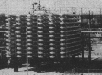
Figure 1-8(b) Tubular reactor photo. Tubular reactor for production of Dimersol G. (Photo courtesy of Editions Techniq Institut Français du Pétrole.)
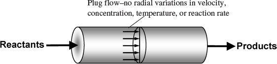
In the tubular reactor, the reactants are continually consumed as they flow down the length of the reactor. In modeling the tubular reactor, we assume that the concentration varies continuously in the axial direction through the reactor. Consequently, the reaction rate, which is a function of concentration for all but zero-order reactions (cf. Equation 3-2), will also vary axially For the purposes of the material presented here, we consider systems in which the flow field may be modeled by that of a plug-flow profile (e.g., uniform velocity
Also see http://encyclopedia.ehe.engin.umich.edu/Pages/Reactors/PFR/PFR.html.
as in turbulent flow), as shown in Figure 1-9. That is, there is no radial variation in reaction rate, and the reactor is referred to as a plug-flow reactor (PFR). (The laminar-flow reactor is discussed in PDF Chapters 16 through 18 and on the Web site, along with a discussion of nonideal reactors.)
Also see PRS and Visual Encyclopedia of Equipment.
The general mole balance equation is given by Equation (1-4)
The equation we will use to design PFRs at steady state can be developed in two ways: (1) directly from Equation (1-4) by differentiating with respect to volume V, and then rearranging the result or (2) from a mole balance on species j in a differential segment of the reactor volume ΔV. Let’s choose the second way to arrive at the differential form of the PFR mole balance. The differential volume, ΔV, shown in Figure 1-10, will be chosen sufficiently small such that there are no spatial variations in reaction rate within this volume. Thus the generation term, ΔGj is

Dividing by ΔV and rearranging
the term in brackets resembles the definition of a derivative
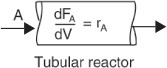
Taking the limit as ΔV approaches zero, we obtain the differential form of steady state mole balance on a PFR
We could have made the cylindrical reactor on which we carried out our mole balance an irregularly shaped reactor, such as the one shown in Figure 1-11 for reactant species A. However, we see that by applying Equation (1-10), the result would yield the same equation (i.e., Equation (1-11)). For species A, the mole balance is
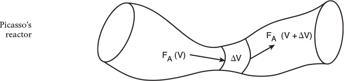
Consequently, we see that Equation (1-11) applies equally well to our model of tubular reactors of variable and constant cross-sectional area, although it is doubtful that one would find a reactor of the shape shown in 1-11 unless it were designed by Pablo Picasso or one of his followers.
The conclusion drawn from the application of the design equation to Picasso’s reactor is an important one: the degree of completion of a reaction achieved in an ideal plug-flow reactor (PFR) does not depend on its shape, only on its total volume.
Again consider the isomerization A → B, this time in a PFR. As the reac-tants proceed down the reactor, A is consumed by chemical reaction and B is produced. Consequently, the molar flow rate FA decreases, while FB increases as the reactor volume V increases, as shown in Figure 1-12.

We now ask, “What is the reactor volume V1 necessary to reduce the entering molar flow rate of A from FA0 to FA1?” Rearranging Equation (1-12) in the form
and integrating with limits at V = 0, then FA = FA0, and at V = V1, then FA = FA1
V1 is the volume necessary to reduce the entering molar flow rate FA0 to some specified value FA1 and also the volume necessary to produce a molar flow rate of B of FB1.
1.4.3 Packed-Bed Reactor (PBR)
The principal difference between reactor design calculations involving homogeneous reactions and those involving fluid-solid heterogeneous reactions is that for the latter, the reaction takes place on the surface of the catalyst (see Figure 10-5). The greater the mass of a given catalyst, the greater the reactive surface area. Consequently, the reaction rate is based on mass of solid catalyst, W, rather than on reactor volume, V. For a fluid-solid heterogeneous system, the rate of reaction of a species A is defined as
The mass of solid catalyst is used because the amount of catalyst is what is important to the rate of product formation. We note that by multiplying the heterogeneous reaction rate, , by the bulk catalyst density, , We can obtain the homogeneous reaction rate, −rA
The reactor volume that contains the catalyst is of secondary significance. Figure 1-13 shows a schematic of an industrial catalytic reactor with vertical tubes packed with solid catalyst.
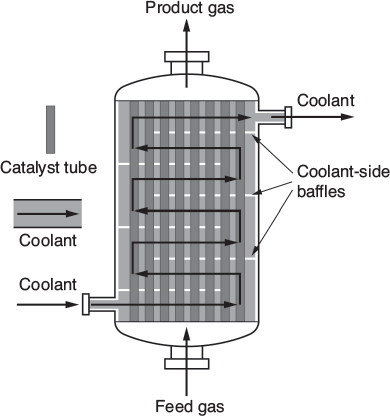
Figure 1-13 Longitudinal catalytic packed-bed reactor. [From Cropley, American Institute of Chemical Engineers, 86(2), 34 (1990).
Also see http://encyclopedia.che.engin.umich.edu/Pages/Reactors/PBR/PBR.html.
In the three idealized types of reactors just discussed (the perfectly mixed batch reactor [BR], the plug-flow tubular reactor [PFR]), and the perfectly mixed continuous-stirred tank reactor [CSTR]), the design equations (i.e., mole balances) were developed based on reactor volume. The derivation of the design equation for a packed-bed catalytic reactor (PBR) will be carried out in a manner analogous to the development of the tubular design equation. To accomplish this derivation, we simply replace the volume coordinate in Equation (1-10) with the catalyst mass (i.e., weight) coordinate W (Figure 1-14).

As with the PFR, the PBR is assumed to have no radial gradients in concentration, temperature, or reaction rate. The generalized mole balance on species A over catalyst weight AW results in the equation
The dimensions of the generation term in Equation (1-14) are
which are, as expected, the same dimensions of the molar flow rate FA. After dividing by ΔW and taking the limit as ΔW → 0, we arrive at the differential Use the differential form of the mole balance for a packed-bed reactor
Use the differential form of design equation for catalyst decay and pressure drop.
When pressure drop through the reactor (see Section 5.5) and catalyst decay (see Section 10.7 in Chapter 10) are neglected, the integral form of the packed-catalyst-bed design equation can be used to calculate the catalyst weight
You can use the integral form only when there is no ΔP and no catalyst decay.
W is the catalyst weight necessary to reduce the entering molar flow rate of species A, FA0, down to a molar flow rate FA.
For some insight into things to come, consider the following example of how one can use the tubular reactor design in Equation (1-11).
Example 1-2 How Large Is the Reactor Volume?
Consider the liquid phase cis – trans isomerization of 2–butene

which we will write symbolically as
A → B
The reaction is first order in A (−rA = kCA) and is carried out in a tubular reactor in which the volumetric flow rate, υ, is constant, i.e., υ = υ0.

1. Sketch the concentration profile.
2. Derive an equation relating the reactor volume to the entering and exiting concentrations of A, the rate constant k, and the volumetric flow rate υ0 .
3. Determine the reactor volume, V1, necessary to reduce the exiting concentration to 10% of the entering concentration, i.e., CA = 0.1 CA0, when the volumetric flow rate υ0 is 10 dm3/min (i.e., liters/min) and the specific reaction rate, k, is 0.23 min−1.
Solution
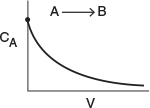
1. Sketch CA as a function of V.
Species A is consumed as we move down the reactor, and as a result, both the molar flow rate of A and the concentration of A will decrease as we move. Because the volumetric flow rate is constant, υ = υ0 , one can use Equation (1-8) to obtain the concentration of A, CA = FA/υ0, and then by comparison with the plot in Figure 1-12, obtain the concentration of A as a function of reactor volume, as shown in Figure E1-2.1.

2. Derive an equation relating V, υ0, k, CA0, and CA.
For a tubular reactor, the mole balance on species A (j = A) was shown to be given by Equation (1-11). Then for species A (j = A)
Mole Balance:
For a first-order reaction, the rate law (discussed in Chapter 3, Eq. (3-5)) is
Rate Law:
Because the volumetric flow rate, υ, is constant (υ = υ0), as it is for most all liquid-phase reactions,
Reactor sizing
Multiplying both sides of Equation (E1-2.2) by minus one and then substituting Equation (E1-2.1) yields
Combine:
Separating the variables and rearranging gives
Using the conditions at the entrance of the reactor that when V = 0, then CA = CA0
Carrying out the integration of Equation (E1-2.4) gives
Solve:
We can also rearrange Equation (E1-2.5) to solve for the concentration of A as a function of reactor volume to obtain
Concentration Profile
3. Calculate V. We want to find the volume, V1, at which for k = 0.23 min−1 and υ0 = 10 dm3/min.
Evaluate:
Substituting CA0, CA, υ0, and k in Equation (E1-2.5), we have
Let’s calculate the volume to reduce the entering concentration to CA = 0.01 CA0. Again using Equation (E1-2.5)
Note: We see that a larger reactor (200 dm3) is needed to reduce the exit concentration to a smaller fraction of the entering concentration (e.g., CA = 0.01 CA0).
We see that a reactor volume of 0.1 m3 is necessary to convert 90% of species A entering into product B for the parameters given.
Analysis: For this irreversible liquid-phase first order reaction (i.e., −rA = kC_) being carried out in a PFR, the concentration of the reactant decreases exponentially down the length (i.e., volume V) of the reactor. The more species A that are consumed and converted to product B, the larger must be the reactor volume V. The purpose of the example was to give a vision of the types of calculations we will be carrying out as we study chemical reaction engineering (CRE).
Example 1-3 Numerical Solutions to Example 1-2 Froblem: How Large is the Reactor Volume?
Now we will turn Example 1-2 into a Living Example Problem (LEP) where we can vary parameters to learn their effect on the volume and/or exit concentrations. We will use Polymath to solve the combined mole balance and rate law for the concentration profile.
We begin by rewriting the mole balance, Equation (E1-2.2), in Polymath notation form
Mole Balances
Rate Law
k = 0.23
v0 = 10
A Polymath tutorial to solve the Ordinary Differential Equations (ODEs) can be found on the Web site (http://www.umich.edu/~elements/5e/tutorials/ODE_Equation_Tutorial.pdf).
The parameter values are k = 0.23 min-1, υο = 10 dm3/s and CA0 = 10 mole/dm3. The initial and final values for the integration wrt the volume V are V = 0 and V = 100 dm3.
The output from the Polymath solution is given in Table E 1-3.1 and the axial concentration profiles from species A and B are shown in Figure E1-3.1.
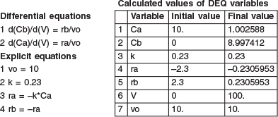

Analysis: Because Polymath will be used extensively in later chapters to solve non-linear ordinary differential equations (ODEs), we introduce it here so that the reader can start to become familiar with it. Figure E1-3.1 shows how the concentrations of species A and B vary down the length of the PFR.
1.5 Industrial Reactors2
Be sure to view the actual photographs of industrial reactors on the CRE Web site. There are also links to view reactors on different Web sites. The CRE Web site also includes a portion of the Visual Encyclopedia of Equipment, encyclopedia.che.engin.umich.edu, “Chemical Reactors” developed by Dr. Susan Montgomery and her students at the University of Michigan. Also see Professional Reference Shelf on the CRE Web site for “Reactors for Liquid-Phase and Gas-Phase Reactions,” along with photos of industrial reactors, and Expanded Material on the CRE Web site.
In this chapter, and on the CRE Web site, we’ve introduced each of the major types of industrial reactors: batch, stirred tank, tubular, and fixed bed (packed bed). Many variations and modifications of these commercial reactors (e.g., semibatch, fluidized bed) are in current use; for further elaboration, refer to the detailed discussion of industrial reactors given by Walas.3
2 Chem. Eng., 63(10), 211 (1956). See also AIChE Modular Instruction Series E, 5 (1984).
3 S. M. Walas, Reaction Kinetics for Chemical Engineers (New York: McGraw-Hill, 1959), Chapter 11.
The CRE Web site describes industrial reactors, along with typical feed and operating conditions. In addition, two solved example problems for Chapter 1 can be found on the CRE Web site, http://www.umich.edu/~elements/5e.
Closure. The goal of this text is to weave the fundamentals of chemical reaction engineering into a structure or algorithm that is easy to use and apply to a variety of problems. We have just finished the first building block of this algorithm: mole balances.
This algorithm and its corresponding building blocks will be developed and discussed in the following chapters:
• Mole Balance, Chapters 1 and 2
• Rate Law, Chapter 3
• Stoichiometry, Chapter 4
• Combine, Chapter 5
• Evaluate, Chapter 5
• Energy Balance, Chapters 11 through 13
With this algorithm, one can approach and solve chemical reaction engineering problems through logic rather than memorization.
Summary
Each chapter summary gives the key points of the chapter that need to be remembered and carried into succeeding chapters.
1. A mole balance on species j, which enters, leaves, reacts, and accumulates in a system volume V, is
If and only if the contents of the reactor are well mixed will the mole balance (Equation (Sl-1)) on species A give
2. The kinetic rate law for rj is
• The rate of formation of species j per unit volume (e.g., mol/s-dm3)
• Solely a function of the properties of reacting materials and reaction conditions (e.g., concentration [activities], temperature, pressure, catalyst, or solvent [if any]) and does not depend on reactor type
• An intensive quantity (i.e., it does not depend on the total amount)
• An algebraic equation, not a differential equation (e.g., −rA = kCA or −rA = kCA2)
For homogeneous catalytic systems, typical units −rj may be gram moles per second per liter; for heterogeneous systems, typical units of may be gram moles per second per gram of catalyst. By convention, −rA is the rate of disappearance of species A and rA is the rate of formation of species A.
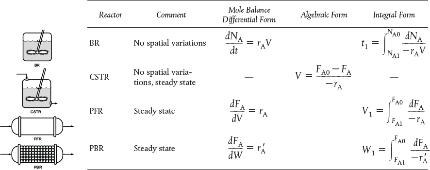
3. Mole balances on species A in four common reactors are shown in Table Sl-1.
TABLE Sl-1 SUMMARY OF REACTOR MOLE BALANCES
CRE Web Site Materials
• Expanded Materials (http://www.umich.edu/~elements/5e/01chap/expanded.html)
1. Industrial Reactors (http://www.umich.edu/~elements/5e/01chap/expanded_ch01.html)
• Learning Resources (http://www.umich.edu/~elements/5e/01chap/learn.html)
1. Summary Notes (http://www.umich.edu/~elements/5e/01chap/summary.html)
2. Self-Tests
A. Exercises (http://www.umich.edu/~elements/5e/01chap/summary-selftest.html)
B. i>clicker Questions
(http://www.umich.edu/-elements/5e/01chap/iclicker_chl_ql.html)
3. Web Material
A. Problem-Solving Algorithm (http://www.umich.edu/~elements/5e/prohsolv/closed/alg/alg.htm)
B. Getting Unstuck on a Problem (http://www.umich.edu/~elements/5e/prohsolv/closed/unstuck/unstuck.html)
C. Smog in L.A. Web module (also see P1-2B) (http://www.umich.edu/~elements/5e/weh_mod/la_hasin/index.htm, includes a Living Example Problem: http://www.umich.edu/~elements/5e/01chap/live.html)
B. Getting Unstuck

C. Smog in L.A.
Fotografiert von ©2002 Hank Good.
3. Interactive Computer Games (http://www.umich.edu/~eiements/5e/icm/index.htmi)
A. Quiz Show I (http://www.umich.edu/~eiements/5e/icm/feinchail.htmi)

4. Solved Problems
A. CDP1-AB Batch Reactor Calculations: A Hint of Things to Come (http://www.umich.edu/-elements/5e/01chap/learn-capl.html)
• FAQ [Frequently Asked Questions]
(http://www.umich.edu/~eiements/5e/01chap/faij.htmi)
• Professional Reference Shelf
R1.1 Photos of Real Reactors
A. http://www.umich.edu/~eiements/5e/01chap/prqf.htmi
B. http://encyclopedia.che.engin.umich.edu/Pages/Reactors/menu.html
R1.2 Reactor Section of the Visual Encyclopedia of Equipment (http://encyclopeiJja.che.engin.umich.eilu/Pages/Reactors/menu.htm!)
This section of the CRE Web site shows industrial equipment and discusses its operation. The reactor portion of this encyclopedia is included on the CRE Web site.
R1.3 Industrial Reactors
(http://umich.edu/~elements/5e/01chap/expanded_ch01.html)
A. Liquid Phase
• Reactor sizes and costs
• Battery of stirred tanks
• Semibatch
B. Gas Phase
• Costs
• Fluidized bed schematic
R1.4 Top-Ten List of Chemical Products and Chemical Companies
(http://umich.edu/~elements/5e/01chap/prof-topten.html)
Questions and Problems
I wish I had an answer for that, because I’m getting tired of answering that question.
—Yogi Berra, New York Yankees Sports Illustrated, June 11, 1984
The subscript to each of the problem numbers indicates the level of difficulty, i.e., A, least difficult; B, moderate difficulty; C, fairly difficult; D, (double black diamond), most difficult. ![]() For example, P1-5B means “1” is the Chapter number, “5” is the problem number, “B” is the problem difficulty, in this case B means moderate difficulty.
For example, P1-5B means “1” is the Chapter number, “5” is the problem number, “B” is the problem difficulty, in this case B means moderate difficulty.
Before solving the problems, state or sketch qualitatively the expected results or trends.
Questions
Q1-1A i>clicker. Go to the Web site (http://www.umich.edu/~elements/5e/01chapliclicker_chl_ql.html) and view at least five i>clicker questions. Choose one that could be used as is, or a variation thereof, to be included on the next exam. You also could consider the opposite case: explaining why the question should not be on the next exam. In either case, explain your reasoning.
Q1-2A Rework Example 1-1 using Equation (3-1), and then compare reaction rates. How do these values compare with those calculated in the example?
Q1-3A In Example 1-2, if the PFR were replaced by a CSTR what would be its volume? Q1-4A Rework Example 1-2 for a constant volume batch reactor to show the time to reduce the number of moles of A to 1% if its initial value is 20 minutes, suggest two ways to work this problem incorrectly.
Q1-5A Read through the Preface. Write a paragraph describing both the content goals and the intellectual goals of the course and text. Also describe what’s on the Web site and how the Web site can be used with the text and course.
Q1-6A View the photos and schematics Chapter 1 Professional Reference Shelf (http://www.umich.edu/~elements/5e/01chap/prof.html). Write a paragraph describing two or more of the reactors. What similarities and differences do you observe between the reactors on the Web (e.g., www.loebequipment.com), on the Web site, and in the text? How do the used reactor prices compare with those in Table 1-1? Q1-7A Critique one of the Learn ChemE Videos for Chapter 1 (http://www.umich.edu/~elements/5e/01chap/learncheme.html) for such things as (a) value, (b) clarity, (c) visuals and (d) how well it held your interest. (Score 1-7; 7 = outstanding, 1= poor)
Q1-8A What assumptions were made in the derivation of the design equation for: (a) The batch reactor (BR)? (b) The CSTR? (c) The plug-flow reactor (PFR)? (d) The packed-bed reactor (PBR)? (e) State in words the meanings of −rA and .
Q1-9A Use the mole balance to derive an equation analogous to Equation (1-7) for a fluidized CSTR containing catalyst particles in terms of the catalyst weight, W, and other appropriate terms.

Computer Simulations and Experiments
P1-1A (a) Revisit Example 1-3.
Wolfram
(i) Describe how CA and CB change when you experiment with varying the volumetric flow rate, υ0, and the specific reaction rate, k, and then write a conclusion about your experiments.
(ii) Click on the description of reversible reaction A ⇆ B to understand how the rate law becomes . Set Ke at its minimum value and vary k and υ0. Next, set Ke at its maximum value and vary k and υ0. Write a couple sentences describing how varying k, v0, and Ke affect the concentration profiles.
(iii) After reviewing Generating Ideas and Solutions on the Web site (http://www.umich.edu/~ele-ments/5e/toc/SCPS,3rdEdBook(Ch07).pdf), choose one of the brainstorming techniques (e.g., lateral thinking) to suggest two questions that should be included in this problem.
Polymath
(iv) Modify the Polymath program to consider the case where the reaction is reversible as discussed in part (ii) above with Ke = 3.
P1-2B Schematic diagrams of the Los Angeles basin are shown in Figure P1-2B. The basin floor covers approximately 700 square miles (2 × 1010 ft2) and is almost completely surrounded by mountain ranges. If one assumes an inversion height in the basin of 2,000 ft, the corresponding volume of air in the basin is 4 × 1013ft3. We shall use this system volume to model the accumulation and depletion of air pollutants. As a very rough first approximation, we shall treat the Los Angeles basin as a well-mixed container (analogous to a CSTR) in which there are no spatial variations in pollutant concentrations.

(http://www.umich.edu/~ekments/5e/web_mod/la_basin/index.htm)
We shall perform an unsteady-state mole balance (Equation (1-4)) on CO as it is depleted from the basin area by a Santa Ana wind. Santa Ana winds are high-velocity winds that originate in the Mojave Desert just to the northeast of Los Angeles. Load the Smog in Los Angeles Basin Web Module. Use the data in the module to work parts 1-12 (a) through (h) given in the module. Load the Living Example Polymath code and explore the problem. For part (i), vary the parameters υ0, a, and b, and write a paragraph describing what you find.
There is heavier traffic in the L.A. basin in the mornings and in the evenings as workers go to and from work in downtown L.A. Consequently, the flow of CO into the L.A. basin might be better represented by the sine function over a 24-hour period.
P1-3B This problem focuses on using Polymath, an ordinary differential equation (ODE) solver, and also a nonlinear equation (NLE) solver. These equation solvers will be used extensively in later chapters. Information on how to obtain and load the Polymath Software is given in Appendix D and on the CRE Web site.
(a) There are initially 500 rabbits (x) and 200 foxes (y) on Professor Sven KöttloVs son-in-law, Stépân Dolez’s, farm near Rica, Jofostan. Use Polymath or MATLAB to plot the concentration of foxes and rabbits as a function of time for a period of up to 500 days. The predator-prey relationships are given by the following set of coupled ordinary differential equations:
Constant for growth of rabbits k1 = 0.02 day-1
Constant for death of rabbits k2 = 0.00004/(day × no. of foxes)
Constant for growth of foxes after eating rabbits k3 = 0.0004/(day x no. of rabbits)
Constant for death of foxes k4 = 0.04 day-1
What do your results look like for the case of k3 = 0.00004/(day × no. of rabbits) and tfinal = 800
days? Also, plot the number of foxes versus the number of rabbits. Explain why the curves look the way they do. Polymath Tutorial (https://www.youtube.com/watch?v=nyjmt6cTiL4)
(b) Using Wolfram in the Chapter 1 LEP on the Web site, what parameters would you change to convert the foxes versus rabbits plot from an oval to a circle? Suggest reasons that could cause this shape change to occur.
(c) We will now consider the situation in which the rabbits contracted a deadly virus. The death rate is rDeath = kDx with feD = 0.005 day-1. Now plot the fox and rabbit concentrations as a function of time and also plot the foxes versus rabbits. Describe, if possible, the minimum growth rate at which the death rate does not contribute to the net decrease in the total rabbit population.
(d) Use Polymath or MATLAB to solve the following set of nonlinear algebraic equations
with inital guesses of x = 2, y = 2. Try to become familiar with the edit keys in Polymath and MATLAB. See the CRE Web site for instructions
Screen shots on how to run Polymath are shown at the end of Summary Notes for Chapter 1 or on the CRE Web site, ivwiv.umich.e<iu/~eIemertts/5e/so/tiv«re/poh’m«tfi-tutorial.html.
Interactive Computer Games
P1-4A Find the Interactive Computer Games (ICG) on the CRE Web site, (http://www.umich.edu/~elements/5e/icg/index.html). Read the description of the Kinetic Challenge module (http://www.umich.edu/~elements/5e/icm/kinchall.html) and then go to the installation instructions (http://www.umich.edu/~elements/5e/icm/install.htmi) to install the module on your computer. Play this game and then record your performance number, which indicates your mastery of the material.
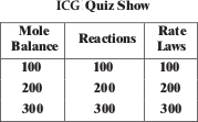
ICG Kinetics Challenge 1 Performance #___________________
Problems
P1-5A The reaction
A + B → 2C
takes place in an unsteady CSTR. The feed is only A and B in equimolar proportions. Which of the following sets of equations gives the correct set of mole balances on A, B, and C? Species A and B are disappearing and species C is being formed. Circle the correct answer where all the mole balances are correct.
(a)
(b)
(c)
(d)
(e) None of the above.
A → B
is to be carried out isothermally in a continuous-flow reactor. The entering volumetric flow rate υ0 is 10 dm3/h. (Note: FA = CAv. For a constant volumetric flow rate υ = υ0, then CAO = FAO/UO = ([5mol/h]/[10dm3/h])0.5mol/dm3.)
Calculate both the CSTR and PFR reactor volumes necessary to consume 99% of A (i.e., when the entering molar flow rate is 5 mol/h, assuming the reaction rate −rA is
(a) −rA = k with [Ans.: VCSTR = 99 dm3]
(b) −rA = kCA with 0.0001 s−1
(c) −rA = kC2A with [Ans.: VCSTR = 660 dm3]
(d) Repeat (a), (b), and/or (c) to calculate the time necessary to consume 99.9% of species A in a 1000 dm3 constant-volume batch reactor with CA0 = 0.5 mol/dm3.
P1-7A Enrico Fermi (1901-1954) Problems (EFP). Enrico Fermi was an Italian physicist who received the Nobel Prize for his work on nuclear processes. Fermi was famous for his “Back of the Envelope Order of Magnitude Calculation” to obtain an estimate of the answer through logic and then to make reasonable assumptions. He used a process to set bounds on the answer by saying it is probably larger than one number and smaller than another, and arrived at an answer that was within a factor of 10. See http://methforam.orj/worfeshops/sum96/tnteriitsc/sheiIa2.htm!.
Enrico Fermi Problem
(a) EFP #1. How many piano tuners are there in the city of Chicago? Show the steps in your reasoning.
1. Population of Chicago___________
2. Number of people per household___________
3. Etc.___________
An answer is given on the CRE Web site under Summary Notes for Chapter 1.
(b) EFP #2. How many square meters of pizza were eaten by an undergraduate student body population of 20,000 during the Fall term 2016?
(c) EFP #3. How many bathtubs of water will the average person drink in a lifetime?
P1-8A What is wrong with this solution? The irreversible liquid phase second order reaction
is carried out in a CSTR. The entering concentration of A, CA0, is 2 molar, and the exit concentration of A, CA is 0.1 molar. The volumetric flow rate, υ0, is constant at 3 dm3/s. What is the corresponding reactor volume?
Solution
1. Mole Balance
2. Rate Law (2nd order)
3. Combine
4.
5.
6.
For more puzzles on what’s “wrong with this solution,” see additional material for each chapter on the CRE Web site home page, under “Expanded Material.”

NOTE TO INSTRUCTORS: Additional problems (cf. those from the preceding editions) can be found in the solutions manual and on the CRE Web site These problems could be photocopied and used to help reinforce the fundamental principles discussed in this chapter.
Supplementary Reading
1. For further elaboration of the development of the general balance equation, see not only the Web site www.umich.edu/~elements/5e/index.html but also
FELDER, R. M., and R. W ROUSSEAU, Elementary Principles of Chemical Processes, 3rd ed. New York: Wiley, 2000, Chapter 4.
SANDERS, R.J., The Anatomy of Skiing. Denver, CO: Golden Bell Press, 1976.
2. A detailed explanation of a number of topics in this chapter can be found in the tutorials.
CRYNES, B. L., and H. S. FOGLER, eds., AlChE Modular Instrudion Series E: Kinetics, Vols. 1 and 2. New York: AIChE, 1981.
3. A discussion of some of the most important industrial processes is presented by
AUSTIN, G. T., Shreve’s Chemical Process Industries, 5th ed. New York: McGraw-Hill, 1984.
4. Short instructional videos (6-9 minutes) that correspond to the topics in this book can be found at http://www.karncfieme.com/.