
9. More Regression Methods
In [1]:
#setup
from mlwpy import *
%matplotlib inline

diabetes = datasets.load_diabetes()

d_tts = skms.train_test_split(diabetes.data,
                              diabetes.target,
                              test_size=.25,
                              random_state=42)

(diabetes_train_ftrs, diabetes_test_ftrs,
 diabetes_train_tgt, diabetes_test_tgt) = d_tts
We are going to dive into a few additional techniques for regression. All of these are variations on techniques we’ve seen before. Two are direct variations on linear regression, one splices a support vector classifier with linear regression to create a Support Vector Regressor, and one uses decision trees for regression instead of classification. As such, much of what we’ll talk about will be somewhat familiar. We’ll also discuss how to build a learner of our own that plugs directly into sklearn’s usage patterns. Onward!
9.1 Linear Regression in the Penalty Box: Regularization
As we briefly discussed in Section 5.4, we can conceptually define the goodness of a model as a cost that has two parts: (1) what we lose, or spend, when we make a mistake and (2) what we invest, or spend, into the complexity of our model. The math is pretty easy here: cost = loss(errors) + complexity. Keeping mistakes low keeps us accurate. If we keep the complexity low, we also keep the model simple. In turn, we also improve our ability to generalize. Overfitting has a high complexity and low training loss. Underfitting has low complexity and high training loss. At our sweet spot, we use just the right amount of complexity to get a low loss on training and testing.
Controlling the complexity term—keeping the complexity low and the model simple—is called regularization. When we discussed overfitting, we talked about some wiggly graphs being too wiggly: they overfit and follow noise instead of pattern. If we reduce some of the wiggliness, we do a better job of following the signal—the interesting pattern—and ignoring the noise.
When we say we want to regularize, or smooth, our model, we are really putting together a few ideas. Data is noisy: it combines noisy distractions with the real useful signal. Some models are powerful enough to capture both signal and noise. We hope that the pattern in the signal is reasonably smooth and regular. If the features of two examples are fairly close to each other, we hope they have similar target values. Excessive jumpiness in the target between two close examples is, hopefully, noise. We don’t want to capture noise. So, when we see our model function getting too jagged, we want to force it back to something smooth.
So, how can we reduce roughness? Let’s restrict ourselves to talking about one type of model: linear regression. I see a raised hand in the back of the classroom. “Yes?” “But Mark, if we are choosing between different straight lines, they all seem to be equally rough!” That’s a fair point. Let’s talk about what it might mean for one line to be simpler than another. You may want to review some of the geometry and algebra of lines from Section 2.6.1. Remember the basic form of a line: y = mx + b. Well, if we get rid of mx, we can have something that is even simpler, but still a line: y = b. A concrete example is y = 3. That is, for any value of x we (1) ignore that value of x—it plays no role now—and (2) just take the value on the right-hand side, 3. There are two ways in which y = b is simpler than y = mx + b:
y = b can only be a 100% correct predictor for a single data point, unless the other target values are cooperative. If an adversary is given control over the target values, they can easily break y = 3 by choosing a second point that has any value besides 3, say 42.
To fully specify a model y = b, I need one value: b. To fully specify a model y = mx + b, I need two values: m and b.
A quick point: if either (1) we set m = 0, getting back to y = b, or (2) we set b = 0 and we get y = mx, we have reduced our capacity to follow true patterns in the data. We’ve simplified the models we are willing to consider. If m = 0, we are literally back to the y = b case: we can only capture one adversarial point. If b = 0, we are in a slightly different scenario, but again, we can only capture one adversarial point. The difference in the second case is that we have an implicit y-intercept—usually specified by an explicit value for b—of zero. Specifically, the line will start at (0, 0) instead of (0, b). In both cases, if we take the zero as a given, we only need to remember one other value. Here’s the key idea: setting weights to zero simplifies a linear model by reducing the number of points it can follow and reducing the number of weights it has to estimate.
Now, what happens when we have more than one input feature? Our linear regression now looks like y = w2x2 + w1x1 + w0. This equation describes a plane in 3D instead of a line in 2D. One way to reduce the model is to pick some ws—say, w1 and w0—and set them to zero. That gives us y = w2x2 which effectively says that we don’t care about the value of x1 and we are content with an intercept of zero. Completely blanking out values seems a bit heavy-handed. Are there more gradual alternatives? Yes, I’m glad you asked.
Instead of introducing zeros, we can ask that the total size of the weights be relatively small. Of course, this constraint brings up problems—or, perhaps, opportunities. We must define total size and relatively small. Fortunately, total hints that we need to add several things up with sum. Unfortunately, we have to pick what we feed to sum.
We want the sum to represent an amount and we want things far away from zero to be counted equally—just as we have done with errors. We’d like 9 and –9 to be counted equally. We’ve dealt with this by (1) squaring values or (2) taking absolute values. As it turns out, we can reasonably use either here.
In [2]:
weights = np.array([3.5, -2.1, .7])
print(np.sum(np.abs(weights)),
      np.sum(weights**2))
6.3 17.15
Now we have to define some criteria for relatively small. Let’s return to our goal: we want to simplify our model to move from overfitting and towards just right. Our just-right values cannot operate on their own, in a vacuum. They must be connected to how well we are fitting the data—we just want to tone down the over part of overfitting. Let’s return to the way we account for the quality of our fit. To investigate, let’s create a bit of data where we specifically control the errors in it:
In [3]:
x_1 = np.arange(10)
m, b = 3, 2
w = np.array([m,b])

x = np.c_[x_1, np.repeat(1.0, 10)] # the plus-one trick

errors = np.tile(np.array([0.0, 1.0, 1.0, .5, .5]), 2)

print(errors * errors)
print(np.dot(errors, errors))

y_true = rdot(w,x)
y_msr  = y_true + errors

D = (x,y_msr)
[0.  1.  1.  0.25  0.25  0.  1.  1. 0.25 0.25]
5.0
Here’s how the truth compares to our noisy data points:
In [4]:
fig, ax = plt.subplots(1,1,figsize=(4,3))
ax.plot(x_1, y_true, 'r', label='true')
ax.plot(x_1, y_msr , 'b', label='noisy')
ax.legend();

Now, I’m going to take a shortcut. I’m not going to go through the process of fitting and finding good parameters from the data. We’re not going to rerun a linear regression to pull out ws (or {m, b}). But imagine that I did and I got back the perfect parameter values—the ones we used to create the data above. Here’s what our sum of squared errors would look like:
In [5]:
def sq_diff(a,b):
        return (a-b)**2
In [6]:
predictions = rdot(w,x)
np.sum(sq_diff(predictions, y_msr))
Out[6]:
5.0
As a reminder, that comes from this equation:
We need to account for our ideas about keeping the weights small. In turn, this constraint is a surrogate for simplifying—regularizing—the model. Let’s say that instead of just making predictions we’ll have a total cost associated with our model. Here goes:
In [7]:
predictions = rdot(w,x)

loss = np.sum(sq_diff(predictions, y_msr))

complexity_1 = np.sum(np.abs(weights))
complexity_2 = np.sum(weights**2) # == np.dot(weights, weights)

cost_1 = loss + complexity_1
cost_2 = loss + complexity_2

print("Sum(abs) complexity:", cost_1)
print("Sum(sqr) complexity:", cost_2)
Sum(abs) complexity: 11.3
Sum(sqr) complexity: 22.15
Remember, we’ve pulled two fast ones. First, we didn’t actually work from the data back to the weights. Instead, we just used the same weights to make the data and to make our not-quite-predictions. Our second fast one is that we used the same weights in both cases, so we have the same losses contributing to both costs. We can’t compare these two: normally, we use one or the other to compute the cost which helps us find a good set of weights under one calculation for loss and complexity.
There’s one last piece I want to introduce before showing a fundamental relationship of learning. Once we define a cost and say that we want to have a low cost, we are really making another tradeoff. I can lower the cost by making fewer errors—leading to a lower loss—or by having less complexity. Am I willing to do both equally or do I consider one more important? Is halving complexity worth doubling the errors I make? Our real goal is trying to make few errors in the future. That happens by making few errors now—on training data—and by keeping model complexity down.
To this end, it is valuable to add a way to trade off towards fewer errors or towards lower complexity. We do that like this:
In [8]:
predictions = rdot(w,x)
errors = np.sum(sq_diff(predictions, y_msr))
complexity_1 = np.sum(np.abs(weights))

C = .5

cost = errors + C * complexity_1
cost
Out[8]:
8.15
Here, I’m saying that as far as cost is concerned, one point of increase in complexity is only worth of a point increase in loss. That is, losses are twice as costly, or twice as important, as complexity. If we use C to represent that tradeoff, we get the following math-heavy equations:
Finding the best line with Cost1 is called L1-regularized regression, or the lasso. Finding the best line with Cost2 is called the L2-regularized regression, or ridge regression.
9.1.1 Performing Regularized Regression
Performing regularized linear regression is no more difficult than the good old-fashioned (GOF) linear regression.
The default value for our C, the total weight of the complexity penalty, is 1.0 for both Lasso and Ridge. In sklearn, the C value is set by the parameter alpha. So, for C = 2, we would call linear_model.Lasso(alpha=2.0). You’ll see λ, α, and C in discussions of regularization; they are all serving a similar role, but you do have to pay attention for authors using slight variations in meaning. For our purposes, we can basically consider them all the same.
In [9]:
models = [linear_model.Lasso(),            # L1 regularized; C=1.0
          linear_model.Ridge()]            # L2 regularized; C=1.0

for model in models:
    model.fit(diabetes_train_ftrs, diabetes_train_tgt)
    train_preds = model.predict(diabetes_train_ftrs)
    test_preds  = model.predict(diabetes_test_ftrs)
    print(get_model_name(model),
          "
Train MSE:",metrics.mean_squared_error(diabetes_train_tgt,
                                                    train_preds),
          "
 Test MSE:", metrics.mean_squared_error(diabetes_test_tgt,
                                                     test_preds))
Lasso
Train MSE: 3947.899897977698
 Test MSE: 3433.1524588051197
Ridge
Train MSE: 3461.739515097773
 Test MSE: 3105.468750907886
Using these is so easy, we might move on without thinking about when and why to use them. Since the default of linear regression is to operate without regularization, we can easily switch to a regularized version and see if it improves matters. We might try that when we train on some data and see an overfitting failure. Then, we can try different amounts of regularization — different values for C — and see what works best on cross-validated runs. We’ll discuss tools to help us pick a C in Section 11.2.
With very noisy data, we might be tempted to make a complex model that is likely to overfit. We have to tolerate a fair bit of error in the model to reduce our complexity. That is, we pay less for complexity and pay a bit more for errors. With noiseless data that captures a linear pattern, we have little need for complexity control and we should see good results with GOF linear regression.
9.2 Support Vector Regression
We’ve introduced the idea of a fundamental tradeoff in learning: our cost comes from both the mistakes and the complexity of our learner. Support Vector Regression (SVR) makes use of this in a same-but-different manner. We regularized GOF linear regression by adding a complexity factor to its loss. We can continue down this path and tweak linear regression even further. We can modify its loss also. Remember: cost = loss + complexity. The standard loss in linear regression is the sum of squared errors called the squared error loss. As we just saw, that form is also called L2—in this case, the L2 loss. So, you might think, “Aha! Let’s use L1, the sum of absolute values.” You are close. We’re going to use L1, but we’re going to tweak it. Our tweak is to use L1 and ignore small errors.
9.2.1 Hinge Loss
In our first look at Support Vector Classifiers (SVCs) from Section 8.3, we didn’t discuss the underlying magic that lets a SVC do its tricks. It turns out that the magic is very similar for the SVC and SVR: both make use of a slightly different loss than linear regression (either kind). In essence, we want to measure what happens when we are wrong and we want to ignore small errors. Putting these two pieces together gives us the idea of the hinge loss. For starters, here’s what the absolute values of the errors look like:
In [10]:
# here, we don't ignore small errors
error = np.linspace(-4, 4, 100)

loss = np.abs(error)

fig, ax = plt.subplots(1,1,figsize=(4,3))
ax.plot(error, loss)

ax.set_xlabel('Raw Error')
ax.set_ylabel('Abs Loss');

How can we ignore errors up to a certain threshold? For example, let’s write code that ignores absolute errors that are less than 1.0:
In [11]:
an_error = .75
abs_error = abs(an_error)
if abs_error < 1.0:
    the_loss = 0.0
else:
    the_loss = abs_error
print(the_loss)
0.0
Now we are going to get fancy. Pay close attention. We can rewrite that with some clever mathematics. Here’s our strategy:
Subtract the threshold value from the absolute error.
If the result is is bigger than zero, keep it. Otherwise, take zero instead.
In [12]:
an_error = 0.75
adj_error = abs(an_error) - 1.0
if adj_error < 0.0:
    the_loss = 0.0
else:
    the_loss = adj_error
print(the_loss)
0.0
Can we summarize that with a single mathematical expression? Look at what happens based on adjusted error. If adj_error < 0.0, we get 0. If adj_error >= 0.0, we get adj_error. Together, those two outcomes are equivalent to taking the bigger value of adj_error or 0. We can do that like:
In [13]:
error = np.linspace(-4, 4, 100)

# here, we ignore errors up to 1.0 by taking bigger value
loss = np.maximum(np.abs(error) - 1.0,
                  np.zeros_like(error))

fig, ax = plt.subplots(1,1,figsize=(4,3))
ax.plot(error, loss)

ax.set_xlabel("Raw Error")
ax.set_ylabel("Hinge Loss");

Mathematically, we encode it like this: loss = max(|error| – threshold, 0). Let’s take one more second to deconstruct it. First, we subtract the amount of error we are willing to ignore from the raw error. If it takes us to a negative value, then maxing against zero will throw it out. For example, if we have an absolute error of .5 (from a raw error of .5 or –.5) and we subtract 1, we end up with an adjusted error of –1.5. Maxing with 0, we take the 0. We’re left with zero—no cost. If you squint your eyes a bit, and turn your head sideways, you might be able to see a pair of doors with hinges at the kinks in the prior graph. That’s where the name for the hinge loss comes from. When we apply the hinge loss around a known target, we get a band where we don’t care about small differences.
In [14]:
threshold = 2.5

xs = np.linspace(-5,5,100)
ys_true = 3 * xs + 2

fig, ax = plt.subplots(1,1,figsize=(4,3))
ax.plot(xs, ys_true)
ax.fill_between(xs, ys_true-threshold, ys_true+threshold,
                color=(1.0,0,0,.25))

ax.set_xlabel('Input Feature')
ax.set_ylabel('Output Target');

Now, imagine that instead of knowing the relationship (the blue line above), we only have some data that came from noisy measurements around that true line:
In [15]:
threshold = 2.5

xs = np.linspace(-5,5,100)
ys = 3 * xs + 2 + np.random.normal(0, 1.5, 100)
fig, ax = plt.subplots(1,1,figsize=(4,3))
ax.plot(xs, ys, 'o',  color=(0,0,1.0,.5))
ax.fill_between(xs, ys_true - threshold, ys_true + threshold,
                color=(1.0,0,0,.25));

We might consider many potential lines to fit this data. However, the band around the central line captures most of the noise in the data and throws all of those small errors out. The coverage of the band is close to perfect—there are only a few points out of 100 that have enough of a mistake to matter. Admittedly, we cheated when we drew this band: we based it on information (the true line) that we normally don’t have available. The central line may remind you of the maximum margin separator in SVCs.
9.2.2 From Linear Regression to Regularized Regression to Support Vector Regression
We can develop a progression from GOF linear regression to regularized regression to support vector regression. At each of the steps, we add or tweak some part of the basic recipe. Using the xs and ys from above, we can define a few terms and see the progression. We’ll image that we estimated the w1 parameter to be 1.3 and we’ll take C = 1.0. Our band of ignorance—the threshold on the amount of error we tolerate—is ε = .25. That’s a baby Greek epsilon.
In [16]:
# hyperparameters for the scenario
C, epsilon = 1.0, .25

# parameters
weights = np.array([1.3])
We can make our predictions from that w and look at the three losses—square-error, absolute, and hinge losses. I won’t use the absolute loss any further—it’s just there for comparison sake.
In [17]:
# prediction, error, loss
predictions = rdot(weights, xs.reshape(-1, 1))
errors = ys - predictions

loss_sse   = np.sum(errors ** 2)
loss_sae   = np.sum(np.abs(errors))
loss_hinge = np.sum(np.max(np.abs(errors) - epsilon, 0))
We can also compute the two complexity penalties we need for L1 and L2 regularization. Note the close similarity to the calculations for the losses, except we calculate the complexity from the weights instead of the errors.
In [18]:
# complexity penalty for regularization
complexity_saw = np.sum(np.abs(weights))
complexity_ssw = np.sum(weights**2)
Finally, we have our total costs:
In [19]:
# cost
cost_gof_regression   = loss_sse   + 0.0
cost_L1pen_regression = loss_sse   + C * complexity_saw
cost_L2pen_regression = loss_sse   + C * complexity_ssw
cost_sv_regression    = loss_hinge + C * complexity_ssw
Now, as that code is written, it only calculates a cost for each type of regression for one set of weights. We would have to run that code over and over—with different sets of weights—to find a good, better, or best set of weights.
Table 9.1 shows the mathematical forms that are buried in that code. If we let and be the sum of absolute values and the sum of squared values, respectively, then we can summarize these in the smaller, more readable form of Table 9.2. Remember, the loss applies to the raw errors. The penalty applies to the parameters or weights.
I want to congratulate. By reading Table 9.2, you can see the fundamental differences between these four regression methods. In reality, we don’t know the right assumptions to choose between learning methods—for example, the discriminant methods or these varied regression methods—so we don’t know whether the noise and underlying complexity of data is going to be best suited to one or another of these techniques. But we skirt around this problem by cross-validating to pick a preferred method for a given dataset. As a practical matter, the choice between these models may depend on outside constraints. For some statistical goals—like significance testing, which we aren’t discussing in this book—we might prefer not using SVR. On very complex problems, we probably don’t even bother with GOF linear regression—although it might be a good baseline comparison. If we have lots of features, we may choose the lasso—L1-penalized—to eliminate features entirely. Ridge has a more moderate approach and reduces—but doesn’t eliminate—features.
Table 9.1 The different mathematical forms for penalized regression and SVR.
Name |
Penalty |
Math |
|---|---|---|
GOF Linear Regression |
None |
|
Lasso |
L1 |
|
Ridge |
L2 |
|
SVR |
L1 |
Table 9.2 Common losses and penalties in regression models.
Name |
Loss |
Penalty |
|---|---|---|
GOF LR |
L1 |
0 |
Lasso (L1-Penalty LR) |
L2 |
L1 |
Ridge (L2-Penalty LR) |
L2 |
L2 |
SVR |
Hinge |
L2 |
9.2.3 Just Do It—SVR Style
There are two main options for SVR in sklearn. We won’t dive into the theory, but you can control different aspects with these two different regressors:
∊-SVR (Greek letter epsilon-SVR): you set the error band tolerance. ν is determined implicitly by this choice. This is what you get with the default parameters to
SVRinsklearn.ν-SVR (Greek letter nu-SVR): you set ν, the proportion of kept support vectors with respect to the total number of examples. ε, the error band tolerance, is determined implicitly by this choice.
In [20]:
svrs = [svm.SVR(),   # default epsilon=0.1
        svm.NuSVR()] # default nu=0.5

for model in svrs:
    preds = (model.fit(diabetes_train_ftrs, diabetes_train_tgt)
                  .predict(diabetes_test_ftrs))
    print(metrics.mean_squared_error(diabetes_test_tgt, preds))
5516.346206774444
5527.520141195904
9.3 Piecewise Constant Regression
All of the linear regression techniques we’ve looked at have one common theme: they assume that a suitably small variation of the inputs will lead to a small variation in the output. You can phrase this in several different ways, but they are all related to the concept of smoothness. The output never jumps around. In classification, we expect the outputs to make leaps: at some critical point we move from predicting dog to predicting cat. Methods like logistic regression have smooth transitions from one class to the next; decision tree classifiers are distinctly dog-or-cat. In mathese, if we have a numerical output value that is not sufficiently smooth, we say we have a discontinuous target.
Let’s draw up a concrete example. Suppose there is a hotdog stand that wants to be cash-only but doesn’t want to deal with coins. They want to be literally paper-cash only. So, when a customer gets a bill of $2.75, they simply round up and charge the customer $3.00. We won’t discuss how the customers feel about this. Here’s a graph that converts the raw bill to a collected bill:
In [21]:
raw_bill = np.linspace(.5, 10.0, 100)
collected = np.round(raw_bill)

fig, ax = plt.subplots(1,1,figsize=(4,3))
ax.plot(raw_bill, collected, '.')
ax.set_xlabel("raw cost")
ax.set_ylabel("bill");

The graph looks a bit like a set of stairs. It simply isn’t possible for our smooth regression lines to capture the pattern in this relationship. A single line through this dataset will have problems. We could connect the fronts of the steps, the backs of the steps, the middles of the steps: none of these will be quite right. We could connect the front of the bottom step to the back of the top step. Again, we still can’t make it work perfectly. If we use GOF linear regression, we’ll capture the middle points fairly well, but the ends of each step will be missed. To put it bluntly, the bias of linear regression puts a fundamental limit on our ability to follow the pattern.
You might be thinking that a decision tree could break down the inputs into little buckets. You’d be completely right—we’ll talk about that in the next section. But I’d like to take a middle ground between using linear regression and modifying decision trees to perform regression. We’re going to do piecewise linear regression in the simplest possible way: with piecewise constant regression. For each region of the input features, we’re going to predict a simple horizontal line. That means we’re predicting a single constant value for that region.
Our raw cost-versus-bill graph was one example where this is an appropriate model. Here’s another example that has a less consistent relationship. Instead of constantly working our way up, we move both up and down as x increases. We start by defining some split points. If we wanted four lines, we’d define three split points (remember, when you cut a rope, you go from one piece of rope to two). Imagine we split at a, b, and c. Then, we’ll fit four lines on the data: (1) from very small up to a, (2) from a to b, (3) from b to c, and (4) from c onwards to very big. Making that slightly more concrete, imagine a,b,c=3,8,12. The result might look like
In [22]:
fig, ax = plt.subplots(1,1,figsize=(4,3))
ax.plot([0,3],   [0,0],
        [3,8],   [5,5],
        [8,12],  [2,2],
        [12,15], [9,9])
ax.set_xticks([3,8,12]);

You might be able to make some educated guesses about how the number of splits relates to bias. If there are no splits, we are simply performing linear regression without a slope—predicting a constant value everywhere using the mean. If we go to the other extreme, we’ll have n data points and make n – 1 mini-lines. Would that model exhibit good training performance? What about applying it to predict on a test set? This model would be great in training, but it would be very bad in testing: it overfits the data.
In some respects, piecewise constant regression is like k-Nearest Neighbors Regression (k-NN-R). However, k-NN-R considers examples based on relative distance instead of raw numeric value. We claim a new testing example is like training examples 3, 17, or 21 because they are close to the new example, regardless of the raw numeric value. Piecewise constant regression gives examples the same target value based on a preset range of splits: I’m like the examples with values between 5 and 10 because my value is 6, even if I’m closer to an example with value 4.
In data science, we use the phrase let the data speak for itself. Here, that idea is front and center: with k-NN-R the data determines the boundary between predictions and those boundaries move with the density of the data. Denser regions get more potential boundaries. With piecewise constant regression, our splits are predetermined. There’s no wiggle room for areas with high or low densities of data. The net effect is that we may do very well when choosing splits for piecewise regression if we have some strong background information about the data. For example, in the US, tax brackets are set by predetermined break points. If we don’t have the right information, our splits may do much worse than k-NN-R.
9.3.1 Implementing a Piecewise Constant Regressor
So far, we’ve only made use of prebuilt models. In the spirit of full disclosure, I snuck in a custom-made diagonal LDA model at the end of the previous chapter, but we didn’t discuss the implementation at all. Since sklearn doesn’t have a built-in piecewise regression capability, we’ll take this as an opportunity to implement a learner of our own. The code to do so is not too bad: it has about 40 lines and it makes use of two main ideas. The first idea is relatively straightforward: to perform each constant regression for the individual pieces, we’ll simply reuse sklearn’s built-in linear regression on a rewritten form of the data. The second idea is that we need to map from the input feature—we’ll limit ourselves to just one for now—to the appropriate section of our rope. This mapping is a bit more tricky, since it has two steps.
Step one involves using np.searchsorted. searchsorted is itself sort of tricky, but we can summarize what it does by saying that it finds an insertion point for a new element into a sorted sequence of values. In other words, it says where someone should enter a line of people ordered by height to maintain the ordering. We want to be able to translate a feature value of 60 to segment, or rope piece, 3. We need to do this in both the training and testing phases.
Step two is that we convert the rope pieces to true/false indicators. So, instead of Piece = 3, we have Piece1 = False, Piece2 = False, Piece3 = True. Then, we learn a regression model from the piece indicators to the output target. When we want to predict a new example, we simply run it through the mapping process to get the right piece indicator and then pipe it to the constant linear regression. The remapping is all wrapped up in the _recode member function in the code below.
9.3.2 General Notes on Implementing Models
The sklearn docs discuss how to implement custom models. We’re going to ignore some of the possible alternatives and lay out a simplified process.
Since we’re implementing a regressor, we’ll inherit from
BaseEstimatorandRegressorMixin.We will not do anything with the model arguments in
__init__.We’ll define
fit(X,y)andpredict(X)methods.We can make use of
check_X_yandcheck_arrayto verify arguments are valid in thesklearnsense.
Two quick comments on the code:
The following code only works for a single feature. Extending it to multiple features would be a fun project. We’ll see some techniques in Chapter 10 that might help.
If no cut points are specified, we use one cut point for every ten examples and we choose the cut points at evenly spaced percentiles of the data.
If we have two regions, the one split would be at 50%, the median. With three or four regions, the splits would be at 33–67% or 25–50–75%. Recall that percentiles are where x% of the data is less than that value. For example, if 50% of our data is less than 5’11”, than 5’11” is the 50th percentile value. Ironically, a single split at 50% might be particularly bad if the data is concentrated in the middle, as might be the case with heights.
In [23]:
from sklearn.base import BaseEstimator, RegressorMixin
from sklearn.utils.validation import (check_X_y,
                                      check_array,
                                      check_is_fitted)

class PiecewiseConstantRegression(BaseEstimator, RegressorMixin):
    def __init__(self, cut_points=None):
       self.cut_points = cut_points

    def fit(self, X, y):
        X, y = check_X_y(X,y)
        assert X.shape[1] == 1 # one variable only

        if self.cut_points is None:
            n = (len(X) // 10) + 1
            qtiles = np.linspace(0.0, 1.0, n+2)[1:-1]
            self.cut_points = np.percentile(X, qtiles, axis=1)
        else:
            # ensure cutpoints in order and in range of X
            assert np.all(self.cut_points[:-1] < self.cut_points[1:])
            assert (X.min() < self.cut_points[0] and
                    self.cut_points[-1] < X.max())

        recoded_X = self._recode(X)
        # even though the _inner_ model is fit without an intercept,
        # our piecewise model *does* have a constant term (but see notes)
        self.coeffs_ = (linear_model.LinearRegression(fit_intercept=False)
                                    .fit(recoded_X, y).coef_)
    def _recode(self, X):
        cp = self.cut_points
        n_pieces = len(cp) + 1
        recoded_X = np.eye(n_pieces)[np.searchsorted(cp, X.flat)]
        return recoded_X

    def predict(self, X):
        check_is_fitted(self, 'coeffs_')
        X = check_array(X)
        recoded_X = self._recode(X)
        return rdot(self.coeffs_, recoded_X)
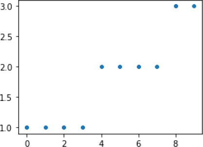
To test and demonstrate that code, let’s generate a simple example dataset we can train on.
In [24]:
ftr = np.random.randint(0,10,(100,1)).astype(np.float64)
cp = np.array([3,7])
tgt = np.searchsorted(cp, ftr.flat) + 1

fig, ax = plt.subplots(1,1,figsize=(4,3))
ax.plot(ftr, tgt, '.');
Since we played by the rules and wrote a learner that plugs directly into the sklearn usage pattern (that’s also called an API or application programming interface), our use of the code will be quite familiar.
In [25]:
# here, we're giving ourselves all the help we can by using
# the same cut points as our data were generated with
model = PiecewiseConstantRegression(cut_points=np.array([3, 7]))
model.fit(ftr, tgt)
preds = model.predict(ftr)
print("Predictions equal target?", np.allclose(preds, tgt))
Predictions equal target? True
As written, PiecewiseConstantRegression is defined by some hyperparameters (the cut points) and some parameters (the constants associated with each piece). The constants are computed when we call fit. The overall fit of the model is very, very sensitive to the number and location of the split points. If we are thinking about using piecewise methods, we either (1) hope to have background knowledge about where the jumps are or (2) are willing to spend time trying different hyperparameters and cross-validating the results to get a good end product.
Now, even though I’m taking the easy way out and talking about piecewise constants—the individual lines have a b but no mx—we could extend this to piecewise lines, piecewise parabolas, etc. We could also require that the end points meet. This requirement would get us a degree of continuity, but not necessarily smoothness. Phrased differently, we could connect the piecewise segments but there might still be sharp turns. We could enforce an even higher degree of smoothness where the turns have to be somewhat gentle. Allowing more bends in the piecewise components reduces our bias. Enforcing constraints on the meeting points regularizes—smooths—the model.
9.4 Regression Trees
One of the great aspects of decision trees is their flexibility. Since they are conceptually straightforward—find regions with similar outputs, label everything in that region in some way—they can be easily adapted to other tasks. In case of regression, if we can find regions where a single numerical value is a good representation of the whole region, we’re golden. So, at the leaves of tree, instead of saying cat or dog, we say 27.5.
9.4.1 Performing Regression with Trees
Moving from piecewise constant regression to decision trees is a straightforward conceptual step. Why? Because you’ve already done the heavy lifting. Decision trees give us a way to zoom in on regions that are sufficiently similar and, having selected a region, we predict a constant. That zoom-in happens as we segment off regions of space.
Eventually, we get to a small enough region that behaves in a nicely uniform way. Basically, using decision trees for regression gives us an automatic way of picking the number and location of split points. These splits are determined by computing the loss when a split breaks the current set of data at a node into two subsets. The split that leads to the immediate lowest squared error is the chosen breakpoint for that node. Remember that tree building is a greedy process and it is not guaranteed to be a globally best step—but a sequence of greedy steps is often good enough for day-to-day use.
In [26]:
dtrees = [tree.DecisionTreeRegressor(max_depth=md) for md in [1, 3, 5, 10]]

for model in dtrees:
    preds = (model.fit(diabetes_train_ftrs, diabetes_train_tgt)
                  .predict(diabetes_test_ftrs))
    mse = metrics.mean_squared_error(diabetes_test_tgt, preds)
    fmt = "{} {:2d} {:4.0f}"
    print(fmt.format(get_model_name(model),
                     model.get_params()['max_depth'],
                     mse))
DecisionTreeRegressor  1 4341
DecisionTreeRegressor  3 3593
DecisionTreeRegressor  5 4312
DecisionTreeRegressor 10 5190
Notice how adding depth helps and then hurts. Let’s all say it together: overfitting! If we allow too much depth, we split the data into too many parts. If the data is split too finely, we make unneeded distinctions, we overfit, and our test error creeps up.
9.5 Comparison of Regressors: Take Three
We’ll return to the student dataset and apply some of our fancier learners to it.
In [27]:
student_df = pd.read_csv('data/portugese_student_numeric.csv')
student_ftrs = student_df[student_df.columns[:-1]]
student_tgt  = student_df['G3']
In [28]:
student_tts = skms.train_test_split(student_ftrs, student_tgt)

(student_train_ftrs, student_test_ftrs,
 student_train_tgt,  student_test_tgt) = student_tts
We’ll pull in the regression methods we introduced in Chapter 7:
In [29]:
old_school = [linear_model.LinearRegression(),
              neighbors.KNeighborsRegressor(n_neighbors=3),
              neighbors.KNeighborsRegressor(n_neighbors=10)]
and add some new regressors from this chapter:
In [30]:
# L1, L2 penalized (abs, sqr), C=1.0 for both
penalized_lr = [linear_model.Lasso(),
                linear_model.Ridge()]

# defaults are epsilon=.1 and nu=.5, respectively
svrs = [svm.SVR(), svm.NuSVR()]

dtrees = [tree.DecisionTreeRegressor(max_depth=md) for md in [1, 3, 5, 10]]

reg_models = old_school + penalized_lr + svrs + dtrees
We’ll compare based on root mean squared error (RMSE):
In [31]:
def rms_error(actual, predicted):
    ' root-mean-squared-error function '
    # lesser values are better (a<b means a is better)
    mse = metrics.mean_squared_error(actual, predicted)
    return np.sqrt(mse)
rms_scorer = metrics.make_scorer(rms_error)
and we’ll standardize the data before we apply our models:
In [32]:
scaler = skpre.StandardScaler()

scores = {}
for model in reg_models:
    pipe = pipeline.make_pipeline(scaler, model)
    preds = skms.cross_val_predict(pipe,
                                   student_ftrs, student_tgt,
                                   cv=10)
    key = (get_model_name(model) +
           str(model.get_params().get('max_depth', "")) +
           str(model.get_params().get('n_neighbors', "")))
    scores[key] = rms_error(student_tgt, preds)

df = pd.DataFrame.from_dict(scores, orient='index').sort_values(0)
df.columns=['RMSE']
display(df)
|
RMSE |
|---|---|
DecisionTreeRegressor1 |
4.3192 |
Ridge |
4.3646 |
LinearRegression |
4.3653 |
NuSVR |
4.3896 |
SVR |
4.4062 |
DecisionTreeRegressor3 |
4.4298 |
Lasso |
4.4375 |
KNeighborsRegressor10 |
4.4873 |
DecisionTreeRegressor5 |
4.7410 |
KNeighborsRegressor3 |
4.8915 |
DecisionTreeRegressor10 |
5.3526 |
For the top four models, let’s see some details about performance on a fold-by-fold basis.
In [33]:
better_models = [tree.DecisionTreeRegressor(max_depth=1),
                 linear_model.Ridge(),
                 linear_model.LinearRegression(),
                 svm.NuSVR()]
fig, ax = plt.subplots(1, 1, figsize=(8,4))
for model in better_models:
    pipe = pipeline.make_pipeline(scaler, model)
    cv_results = skms.cross_val_score(pipe,
                                      student_ftrs, student_tgt,
                                      scoring = rms_scorer,
                                      cv=10)

    my_lbl = "{:s} ({:5.3f}$pm${:.2f})".format(get_model_name(model),
                                                cv_results.mean(),
                                                cv_results.std())
    ax.plot(cv_results, 'o--', label=my_lbl)
    ax.set_xlabel('CV-Fold #')
    ax.set_ylabel("RMSE")
    ax.legend()

Each of these goes back and forth a bit. They are all very close in learning performance. The range of the means (4.23, 4.29) is not very wide and it’s also a bit less than the standard deviation. There’s still work that remains to be done. We didn’t actually work through different values for regularization. We can do that by hand, in a manner similar to the complexity curves we saw in Section 5.7.2. However, we’ll approach that in a much more convenient fashion in Section 11.2.
9.6 EOC
9.6.1 Summary
At this point, we’ve added a number of distinctly different regressors to our quiver of models. Decision trees are highly flexible; regularized regression and SVR update the linear regression to compete with the cool kids.
9.6.2 Notes
We talked about L1 and L2 regularization. There is a method in sklearn called ElasticNet that allows us to blend the two together.
While we were satisfied with a constant-value prediction for each region at the leaf of a tree, we could—standard methods don’t—make mini-regression lines (or curves) at each of the leaves.
Trees are one example of an additive model. Classification trees work by (1) picking a region and (2) assigning a class to examples from that region. If we pick one and only one region for each example, we can write that as a peculiar sum, as we did in Section 8.2.1. For regression, it is a sum over region selection and target value. There are many types of models that fall under the additive model umbrella—such as the piecewise regression line we constructed, a more general version of piecewise regression called splines, and more complicated friends. Splines are interesting because advanced variations of splines can move the choice of decision points from a hyperparameter to a parameter: the decision points become part of the best solution instead of an input. Splines also have nice ways of incorporating regularization—there it is generally called smoothness.
Speaking of smoothness, continuity, and discontinuity: these topics go very, very deep. I’ve mostly used smoothness in an everyday sense. However, in math, we can define smoothness in many different ways. As a result, in mathematics, some continuous functions might not be smooth. Smoothness can be an additional constraint, beyond continuity, to make sure functions are very well behaved.
For more details on implementing your own sklearn-compatible learners, see http://scikit-learn.org/stable/developers/contributing.html#rolling-your-own-estimator. Be aware that the class parameters they discuss there are not the model parameters we have discussed. Instead, they are the model hyperparameters. Part of the problem is the double meaning of parameter in computer science (for information passed into a function) and mathematics (for knobs a machine-model adjusts). For more details, see Section 11.2.1.
After we get through Chapter 10—coming up next, stay tuned—we’ll have some additional techniques that would let us do more general piecewise linear regression that works on multiple features.
9.6.3 Exercises
Build a good old-fashioned, ridge, and lasso regression on the same dataset. Examine the coefficients. Do you notice any patterns? What if you vary the amount of regularization to the ridge and lasso?
Create data that represents a step function: from zero to one, it has value of zero; from one to two, it has a value of one; from two to three, it has the value two, and so on. What line is estimated when you fit a good old-fashioned linear regression to it? Conceptually, what happens if you draw a line through the fronts of the steps? What about the backs? Are any of these lines distinctly better from an error or residual perspective?
Here’s a conceptual question. If you’re making a piecewise linear regression, what would it mean for split points to underfit or overfit the data? How would you assess if either is happening? Follow up: what would a complexity curve for piecewise regression look like? What would it assess?
Evaluate the resource usage for the different learners on the student dataset.
Compare the performance of our regression methods on some other datasets. You might look at the digits via
datasets.load_digits.Make a simple, synthetic regression dataset. Examine the effect of different values of ν (
nu) when you build aNuSVR. Try to make some systematic changes to the regression data. Again, vary ν. Can you spot any patterns? (Warning: patterns that arise in 1, 2, or just a few dimensions—that is, with just a few features—may not hold in higher dimensions.)Conceptual question. What would piecewise parabolas look like? What would happen if we require them to connect at the ends of their intervals?