
14. Feature Engineering for Domains: Domain-Specific Learning
In [1]:
# setup
from mlwpy import *
%matplotlib inline

import cv2
In a perfect world, our standard classification algorithms would be provided with data that is relevant, plentiful, tabular (formatted in a table), and naturally discriminitive when we look at it as points in space.
In reality, we may be stuck with data that is
Only an approximation of our target task
Limited in quantity or covers only some of many possibilities
Misaligned with the prediction method(s) we are trying to apply to it
Written as text or images which are decidedly not in an example-feature table
Issues 1 and 2 are specific to a learning problem you are focused on. We discussed issue 3 in Chapters 10 and 13; we can address it by manually or automatically engineering our feature space. Now, we’ll approach issue 4: what happens when we have data that isn’t in a nice tabular form? If you were following closely, we did talk about this a bit in the previous chapter. Through kernel methods, we can make direct use of objects as they are presented to us (perhaps as a string). However, we are then restricted to kernel-compatible learning methods and techniques; what’s worse, kernels come with their own limitations and complexities.
So, how can we convert awkward data into data that plays nicely with good old-fashioned learning algorithms? Though the terms are somewhat hazy, I’ll use the phrase feature extraction to capture the idea of converting an arbitrary data source—something like a book, a song, an image, or a movie—to tabular data we can use with the non-kernelized learning methods we’ve seen in this book. In this chapter, we will deal with two specific cases: text and images. Why? Because they are plentiful and have well-developed methods of feature extraction. Some folks might mention that processing them is also highly lucrative. But, we’re above such concerns, right?
14.1 Working with Text
When we apply machine learning methods to text documents, we encounter some interesting challenges. In contrast to a fixed set of measurements grouped in a table, documents are (1) variable-length, (2) order-dependent, and (3) unaligned. Two different documents can obviously differ in length. While learning algorithms don’t care about the ordering of features—as long as they are in the same order for each example—documents most decidedly do care about order: “the cat in the hat” is very different from “the hat in the cat” (ouch). Likewise, we expect the order of information for two examples to be presented in the same way for each example: feature one, feature two, and feature three. Two different sentences can communicate the same information in many different arrangements of—possibly different—words: “Sue went to see Chris” and “Chris had a visitor named Sue.”
We might try the same thing with two very simple documents that serve as our examples: “the cat in the hat” and “the quick brown fox jumps over the lazy dog”. After removing the super common, low-meaning stop words—like the—we end up with
|
sentence |
|---|---|
example 1 |
cat in hat |
example 2 |
quick brown fox jumps over lazy dog |
Or,
|
word 1 |
word 2 |
word 3 |
word 4 |
|---|---|---|---|---|
example 1 |
cat |
in |
hat |
* |
example 2 |
quick |
brown |
fox |
jumps |
which we would have to extend out to the longest of all our examples. Neither of these feels right. The first really makes no attempt to tease apart any relationships in the words. The second option seems to go both too far and not far enough: everything is broken into pieces, but word 1 in example 1 may have no relationship to word 1 in example 2.
There’s a fundamental disconnect between representing examples as written text and representing them as rows in a table. I see a hand raised in the classroom. “Yes, you in the back?” “Well, how can we represent text in a table?” I’m glad you asked.
Here’s one method:
Gather all of the words in all of the documents and make that list of words the features of interest.
For each document, create a row for the learning example. Row entries indicate if a word occurs in that example. Here, we use - to indicate no and to let the yeses stand out.
|
in |
over |
quick |
brown |
lazy |
cat |
hat |
fox |
dog |
jumps |
|---|---|---|---|---|---|---|---|---|---|---|
example 1 |
yes |
– |
– |
– |
– |
yes |
yes |
– |
– |
– |
example 2 |
– |
yes |
yes |
yes |
yes |
– |
– |
yes |
yes |
yes |
This technique is called bag of words. To encode a document, we take all the words in it, write them down on slips of paper, and throw them in a bag. The benefit here is ease and quickness. The difficulty is that we completely lose the sense of ordering! For example, “Barb went to the store and Mark went to the garage” would be represented in the exact same way as “Mark went to the store and Barb went to the garage”. With that caveat in mind, in life—and in machine learning—we often use simplified versions of complicated things either because (1) they serve as a starting point or (2) they turn out to work well enough. In this case, both are valid reasons why we often use bag-of-words representations for text learning.
We can extend this idea from working with single words—called unigrams—to pairs of adjacent words, called bigrams. Pairs of words give us a bit more context. In the Barb and Mark example, if we had trigrams—three-word phrases—we would capture the distinction of Mark-store and Barb-garage (after the stop words are removed). The same idea extends to n-grams. Of course, as you can imagine, adding longer and longer phrases takes more and more time and memory to process. We will stick with single-word unigrams for our examples here.
If we use a bag-of-words (BOW) representation, we have several different options for recording the presence of a word in a document. Above, we simply recorded yes values. We could have equivalently used zeros and ones or trues and falses. The large number of dashes points out an important practical issue. When we use BOW, the data become very sparse. Clever storage, behind the scenes, can compress that table by only recording the interesting entries and avoiding all of the blank no entries.
If we move beyond a simple yes/no recording scheme, our first idea might be to record counts of occurrences of the words. Beyond that, we might care about normalizing those counts based on some other factors. All of these are brilliant ideas and you are commended for thinking of them. Better yet, they are well known and implemented in sklearn, so let’s make these ideas concrete.
14.1.1 Encoding Text
Here are a few sample documents that we can use to investigate different ways of encoding text:
In [2]:
docs = ["the cat in the hat",
        "the cow jumped over the moon",
        "the cat mooed and the cow meowed",
        "the cat said to the cow cow you are not a cat"]
To create our features of interest, we need to record all of the unique words that occur in the entire corpus. Corpus is a term for the entire group of documents we are considering.
In [3]:
vocabulary = set(" ".join(docs).split())
We can remove some words that are unlikely to help us. These throwaway words are called stop words. After we remove them, we are left with our vocabulary of words that show up in the corpus.
In [4]:
common_words = set(['a', 'to', 'the', 'in', 'and', 'are'])
vocabulary = vocabulary - common_words
print(textwrap.fill(str(vocabulary)))
{'cow', 'not', 'cat', 'moon', 'jumped', 'meowed', 'said', 'mooed',
'you', 'over', 'hat'}
14.1.1.1 Binary Bags of Words
With our vocabulary in place, some quick MacGyver-ing with Python gets us a simple yes/no table of words in documents. The key test is the w in d that asks if a word is in a document.
In [5]:
# {k:v for k in lst} creates a dictionary from keys:values
# it is called a "dictionary comprehension"
doc_contains = [{w:(w in d) for w in vocabulary} for d in docs]
display(pd.DataFrame(doc_contains))
|
cat |
cow |
hat |
jumped |
meowed |
mooed |
moon |
not |
over |
said |
you |
|---|---|---|---|---|---|---|---|---|---|---|---|
0 |
True |
False |
True |
False |
False |
False |
False |
False |
False |
False |
False |
1 |
False |
True |
False |
True |
False |
False |
True |
False |
True |
False |
False |
2 |
True |
True |
False |
False |
True |
True |
False |
False |
False |
False |
False |
3 |
True |
True |
False |
False |
False |
False |
False |
True |
False |
True |
True |
14.1.1.2 Bag-of-Word Counts
A tiny alteration to the first line of code gives us the counts of words in documents:
In [6]:
word_count = [{w:d.count(w) for w in vocabulary} for d in docs]
wcs = pd.DataFrame(word_count)
display(wcs)
|
cat |
cow |
hat |
jumped |
meowed |
mooed |
moon |
not |
over |
said |
you |
|---|---|---|---|---|---|---|---|---|---|---|---|
0 |
1 |
0 |
1 |
0 |
0 |
0 |
0 |
0 |
0 |
0 |
0 |
1 |
0 |
1 |
0 |
1 |
0 |
0 |
1 |
0 |
1 |
0 |
0 |
2 |
1 |
1 |
0 |
0 |
1 |
1 |
0 |
0 |
0 |
0 |
0 |
3 |
2 |
2 |
0 |
0 |
0 |
0 |
0 |
1 |
0 |
1 |
1 |
sklearn gives us this capability with CountVectorizer.
In [7]:
import sklearn.feature_extraction.text as sk_txt
sparse = sk_txt.CountVectorizer(stop_words='english').fit_transform(docs)
sparse
Out[7]:
<4x8 sparse matrix of type '<class 'numpy.int64'>'
 with 12 stored elements in Compressed Sparse Row format>
As I mentioned, since the data is sparse and sklearn is clever, the underlying machinery is saving us space. If you really want to see what’s going on, turn a sparse form into a dense form with todense:
In [8]:
sparse.todense()
Out[8]:
matrix([[1, 0, 1, 0, 0, 0, 0, 0],
        [0, 1, 0, 1, 0, 0, 1, 0],
        [1, 1, 0, 0, 1, 1, 0, 0],
        [2, 2, 0, 0, 0, 0, 0, 1]], dtype=int64)
We see some slightly different results here because sklearn uses a few more stop words: you, not, and over are in the default English stop word list. Also, it’s not obvious what the ordering of the words is in the sklearn output. But, it’s all there.
14.1.1.3 Normalized Bag-of-Word Counts: TF-IDF
As we’ve seen in many cases—from means to covariances to error rates—we often normalize results so they are compared against some sort of baseline or other standard. In the case of word counts, there are two things we would like to balance:
We don’t want longer documents to have stronger relationships with our target just because they have more words.
If words are frequent in every document, they no longer become a distinguishing factor. So, as frequency of a word increases across the corpus, we’d like the contribution of that word to drop.
Let’s start by accounting for the frequency across all of the documents. We can compute that corpus-wide frequency by asking, “How many documents contain our word?” We can implement that as
In [9]:
# wcs.values.sum(axis=0, keepdims=True)
doc_freq = pd.DataFrame(wcs.astype(np.bool).sum(axis='rows')).T
display(doc_freq)
|
cat |
cow |
hat |
jumped |
meowed |
mooed |
moon |
not |
over |
said |
you |
|---|---|---|---|---|---|---|---|---|---|---|---|
0 |
3 |
3 |
1 |
1 |
1 |
1 |
1 |
1 |
1 |
1 |
1 |
Now, we’re going to take a small leap and go from a corpus frequency to an inverse frequency. Normally, that means we would do something like . However, the usual way this is done in text learning is a bit more complicated: we account for the number of documents and we take the logarithm of the value. Our formula for inverse-document frequency will be .
Why take the log? Logarithms have a magnifying and dilating effect. Basically, taking the log of values greater than one—such as a positive number of documents—compresses the difference between values, while taking the log of values between zero and one—such as one divided by a count—expands the spacing. So, the log here amplifies the effect of different counts and suppresses the value of more and more documents. The number of documents in the numerator serves as a baseline value from which we adjust down.
In [10]:
idf = np.log(len(docs) / doc_freq)
#  == np.log(len(docs)) - np.log(doc_freq)
display(idf)
|
cat |
cow |
hat |
jumped |
meowed |
mooed |
moon |
not |
over |
said |
you |
|---|---|---|---|---|---|---|---|---|---|---|---|
0 |
0.29 |
0.29 |
1.39 |
1.39 |
1.39 |
1.39 |
1.39 |
1.39 |
1.39 |
1.39 |
1.39 |
With this calculation, it’s an easy step to create the term frequency-inverse document frequency, or TF-IDF. All we do is weight each word count by its respective IDF value. Done.
In [11]:
tf_idf  = wcs * idf.iloc[0]   # aligns columns for multiplication
display(tf_idf)
|
cat |
cow |
hat |
jumped |
meowed |
mooed |
moon |
not |
over |
said |
you |
|---|---|---|---|---|---|---|---|---|---|---|---|
0 |
0.29 |
0.00 |
1.39 |
0.00 |
0.00 |
0.00 |
0.00 |
0.00 |
0.00 |
0.00 |
0.0000 |
1 |
0.00 |
0.29 |
0.00 |
1.39 |
0.00 |
0.00 |
1.39 |
0.00 |
1.39 |
0.00 |
0.0000 |
2 |
0.29 |
0.29 |
0.00 |
0.00 |
1.39 |
1.39 |
0.00 |
0.00 |
0.00 |
0.00 |
0.0000 |
3 |
0.58 |
0.58 |
0.00 |
0.00 |
0.00 |
0.00 |
0.00 |
1.39 |
0.00 |
1.39 |
1.39 |
Now, we haven’t accounted for the unwanted benefits that longer documents might get. We can keep them under control by insisting that the total values across a document—when we add up all the weighted counts—be the same. This means documents are differentiated by the proportion of a fixed weight distributed over the word buckets, instead of the total amount across the buckets (which is now the same for everyone). We can do that with Normalizer.
In [12]:
skpre.Normalizer(norm='l1').fit_transform(wcs)
Out[12]:
array([[0.5   , 0.    , 0.5   , 0.    , 0.   , 0.   , 0.    , 0.    ,
        0.    , 0.    , 0.   ],
       [0.    , 0.25  , 0.    , 0.25  , 0.   , 0.   , 0.25  , 0.    ,
        0.25  , 0.    , 0.   ],
       [0.25  , 0.25  , 0.    , 0.    , 0.25 , 0.25 , 0.    , 0.    ,
        0.    , 0.    , 0.   ],
       [0.2857, 0.2857, 0.    , 0.    , 0.   , 0.   , 0.    , 0.1429,
        0.    , 0.1429, 0.1429]])
The sum across a row is now 1.0.
Our process mimics—inexactly—the same steps that sklearn performs with TfidfVectorizer. We won’t try to reconcile our manual steps with the sklearn method; just remember that, at a minimum, we are using different stop words which affects the weightings used for the IDF weights.
In [13]:
sparse = (sk_txt.TfidfVectorizer(norm='l1', stop_words='english')
                .fit_transform(docs))
sparse.todense()
Out[13]:
matrix([[0.3896, 0.    , 0.6104, 0.    , 0.    , 0.    , 0.    , 0.    ],
        [0.    , 0.2419, 0.    , 0.379 , 0.    , 0.    , 0.379 , 0.    ],
        [0.1948, 0.1948, 0.    , 0.    , 0.3052, 0.3052, 0.    , 0.    ],
        [0.3593, 0.3593, 0.    , 0.    , 0.    , 0.    , 0.    , 0.2814]])
14.1.2 Example of Text Learning
To put these ideas into practice, we need a legitimate body of preclassified documents. Fortunately, sklearn has tools to get it for us. The data is not installed with your sklearn distribution; instead, you need to import and call a utility that will download it. The following import will do the necessary steps.
In [14]:
from sklearn.datasets import fetch_20newsgroups
twenty_train = fetch_20newsgroups(subset='train')
The Twenty Newsgroups dataset consists of about 20,000 documents from 20 old-school Internet newsgroups. Newsgroups are a type of online forum that acts a bit like an email thread that multiple people can participate in at once. There are newsgroups for many different discussion topics: religion and politics are always particularly spicy, but there are groups for various sports, hobbies, and other interests. The classification problem is to take an arbitrary document and determine which discussion group it came from.
In [15]:
print("the groups:")
print(textwrap.fill(str(twenty_train.target_names)))
the groups:
['alt.atheism', 'comp.graphics', 'comp.os.ms-windows.misc',
'comp.sys.ibm.pc.hardware', 'comp.sys.mac.hardware', 'comp.windows.x',
'misc.forsale', 'rec.autos', 'rec.motorcycles', 'rec.sport.baseball',
'rec.sport.hockey', 'sci.crypt', 'sci.electronics', 'sci.med',
'sci.space', 'soc.religion.christian', 'talk.politics.guns',
'talk.politics.mideast', 'talk.politics.misc', 'talk.religion.misc']
The actual contents of the examples are text emails including the header portion with a sender, receiver, and a subject. Here are the first ten lines of the first example:
In [16]:
print("
".join(twenty_train.data[0].splitlines()[:10]))
From: [email protected] (where's my thing)
Subject: WHAT car is this!?
Nntp-Posting-Host: rac3.wam.umd.edu
Organization: University of Maryland, College Park
Lines: 15

 I was wondering if anyone out there could enlighten me on this car I saw
the other day. It was a 2-door sports car, looked to be from the late 60s/
early 70s. It was called a Bricklin. The doors were really small. In addition,
the front bumper was separate from the rest of the body. This is
Once we have the data available, we can almost instantly apply the TF-IDF transformer to get a useful representation of our documents.
In [17]:
ct_vect     = sk_txt.CountVectorizer()
tfidf_xform = sk_txt.TfidfTransformer()

docs_as_counts = ct_vect.fit_transform(twenty_train.data)
docs_as_tfidf  = tfidf_xform.fit_transform(docs_as_counts)
We can connect that data to any of our learning models. Here we use a variant of Naive Bayes:
In [18]:
model = naive_bayes.MultinomialNB().fit(docs_as_tfidf,
                                        twenty_train.target)
Now, you might ask if we can take all these steps and wrap them up in a pipeline. Of course we can!
In [19]:
doc_pipeline = pipeline.make_pipeline(sk_txt.CountVectorizer(),
                                      sk_txt.TfidfTransformer(),
                                      naive_bayes.MultinomialNB())
Before we ramp up for evaluation, let’s reduce the number of categories we consider:
In [20]:
categories = ['misc.forsale',
              'comp.graphics',
              'sci.med',
              'sci.space']
We can even go one step better. TfidfVectorizer combines the two preprocessing, feature-extracting steps in one component. So, here is a super compact approach to this problem:
In [21]:
twenty_train = fetch_20newsgroups(subset='train',
                                  categories=categories,
                                  shuffle=True,
                                  random_state=42)

doc_pipeline = pipeline.make_pipeline(sk_txt.TfidfVectorizer(),
                                      naive_bayes.MultinomialNB())

model = doc_pipeline.fit(twenty_train.data, twenty_train.target)
And we can quickly evaluate the quality of our model:
In [22]:
twenty_test = fetch_20newsgroups(subset='test',
                                 categories=categories,
                                 shuffle=True,
                                 random_state=42)

doc_preds = model.predict(twenty_test.data)
cm = metrics.confusion_matrix(twenty_test.target, doc_preds)
ax = sns.heatmap(cm, annot=True,
                 xticklabels=twenty_test.target_names,
                 yticklabels=twenty_test.target_names,
                 fmt='3d') # cells are counts
ax.set_xlabel('Predicted')
ax.set_ylabel('Actual');
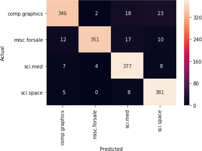
I hope that makes you smile. We’ve done a lot of work to get to this point. We are now putting together (1) feature engineering in the form of feature extraction from text documents to an example-feature table, (2) building a learning model from training data, and (3) looking at the evaluation of that model on separate testing data—all in about 25 lines of code over the last two code cells. Our results don’t look too bad, either. Hopefully, you understand something about each of that steps we’ve just accomplished.
14.2 Clustering
Shortly, we are going to discuss some techniques to use for classifying images. One large component in that process is clustering. So, let’s take a few minutes to describe clustering.
Clustering is a method of grouping similar examples together. When we cluster, we don’t make an explicit appeal to some known target value. Instead, we have some preset standard that we use to decide what is the same and what is different in our examples. Just like PCA, clustering is an unsupervised learning technique (see Section 13.3). PCA maps examples to some linear thing (a point, line, or plane); clustering maps examples to groups.
14.2.1 k-Means Clustering
There are a number of ways to perform clustering. We will focus on one called k-Means Clustering (k-MC). The idea of k-Means Clustering is that we assume there are k groups each of which has a distinct center. We then try to partition the examples into those k groups.
It turns out that there is a pretty simple process to extract out the groups:
Randomly pick k centers.
Assign examples to groups based on the closest center.
Recompute the centers from the assigned groups.
Return to step 2.
Eventually, this process will result in only very small changes to the centers. At that point, we can say we have converged on a good answer. Those centers form the foundations of our groups.
While we can use clustering without a known target, if we happen to have one we can compare our clustered results with reality. Here’s an example with the iris dataset. To make a convenient visualization, we’re going to start by using PCA to reduce our data to two dimensions. Then, in those two dimensions, we can look at where the actual three varieties of iris fall. Finally, we can see the clusters that we get by using k-MC.
In [23]:
iris = datasets.load_iris()
twod_iris = (decomposition.PCA(n_components=2, whiten=True)
                          .fit_transform(iris.data))
clusters = cluster.KMeans(n_clusters=3).fit(twod_iris)

fig, axes = plt.subplots(1,2,figsize=(8,4))
axes[0].scatter(*twod_iris.T, c=iris.target)
axes[1].scatter(*twod_iris.T, c=clusters.labels_)

axes[0].set_title("Truth"), axes[1].set_title("Clustered");

You’ll quickly notice that k-MC split the two mixed species the wrong way—in reality they were split more vertically, but k-MC split them horizontally. Without the target value—the actual species—to distinguish the two, the algorithm doesn’t have any guidance about the right way to tell apart the intertwined species. More to the point, in clustering, there is no definition of right. The standard is simply defined by how the algorithm operates.
Although sklearn doesn’t currently provide them as off-the-shelf techniques, k-MC and other clustering techniques can be kernelized in the same fashion as the methods we discussed in Section 13.2. In the next section, we are going to use clusters to find and define synonyms of visual words to build a global vocabulary across different local vocabularies. We will group together different local words that mean approximately the same thing into single, representative global words.
14.3 Working with Images
There are many, many ways to work with images that enable learners to classify them. We’ve talked about using kernels for nontabular data. Clever folks have created many ways to extract features from raw image pixels. More advanced learning techniques—like deep neural networks—can build very complicated, useful features from images. Whole books are available on these topics; we can’t hope to cover all of that ground. Instead, we are going to focus on one technique that very nicely builds from the two prior topics in the chapter: bags of words and clustering. By using these two techniques in concert, we will be able to build a powerful feature extractor that will transform our images from a grid of pixels into a table of usable and useful learning features.
14.3.1 Bag of Visual Words
We have an overall strategy that we want to implement. We want to—somehow—mimic the bag-of-words approach that we used in text classification, but with images. Since we don’t have literal words, we need to come up with some. Fortunately, there’s a very elegant way to do that. I’ll give you a storytime view of the process and then we’ll dive into the details.
Imagine you are at a party. The party is hosted at an art museum, but it is attended by people from all walks of life and from all over the world. The art museum is very large: you have no hope of checking out every painting. But, you stroll around for a while and start developing some ideas about what you like and what you don’t like. After a while, you get tired and head to the cafe for some refreshments. As you sip your refreshing beverage, you notice that there are other folks, also tired, sitting around you. You wonder if they might have some good recommendations as to what other paintings you should check out.
There are several levels of difficulty in getting recommendations. All of the attendees have their own likes and dislikes about art; there are many different, simple and sophisticated, ways of describing those preferences; and many of the attendees speak different languages. Now, you could mill around and get a few recommendations from those people who speak your language and seem to describe their preferences in a way that makes sense to you. But imagine all the other information you are missing out on! If there were a way we could translate all of these individual vocabularies into a group vocabulary that all the attendees could use to describe the paintings, then we could get everyone to see paintings that they might enjoy.
The way we will attack this problem is by combining all of the individual vocabularies and grouping them into synonyms. Then, every term that an individual would use to describe a painting can be translated into the global synonym. For example, all terms that are similar to red—scarlet, ruby, maroon—could be translated to the single term red. Once we do this, instead of having dozens of incompatible vocabularies, we have a single group vocabulary that can describe the paintings in common way. We will use this group vocabulary as the basis for our bag of words. Then, we can follow a process much like our text classification to build our learning model.
14.3.2 Our Image Data
We need some data to work with. We are going to make use of the Caltech101 dataset. If you want to play along at home, download and uncompress the data from www.vision.caltech.edu/Image_Datasets/Caltech101/101_ObjectCategories.tar.gz.
There are 101 total categories in the dataset. The categories represent objects in the world, such as cats and airplanes. You’ll see 102 categories below because there are two sets of faces, one hard and one easy.
In [24]:
# exploring the data
objcat_path = "./data/101_ObjectCategories"
cat_paths = glob.glob(osp.join(objcat_path, "*"))
all_categories = [d.split('/')[-1] for d in cat_paths]

print("number of categories:", len(all_categories))
print("first 10 categories:n",
      textwrap.fill(str(all_categories[:10])))
number of categories: 102
first 10 categories:
 ['accordion', 'airplanes', 'anchor', 'ant', 'BACKGROUND_Google',
'barrel', 'bass', 'beaver', 'binocular', 'bonsai']
The data itself is literally graphics files. Here’s an accordion:
In [25]:
from skimage.io import imread

test_path = osp.join(objcat_path, 'accordion', 'image_0001.jpg')
test_img = imread(test_path)

fig, ax = plt.subplots(1,1,figsize=(2,2))
ax.imshow(test_img)
ax.axis('off');

It’s probably a reasonable guess that without some preprocessing—feature extraction—we have little hope of classifying these images correctly.
14.3.3 An End-to-End System
For our learning problem, we have a basket of images and a category they come from. Our strategy to make an end-to-end learning system is shown in Figures 14.1 and 14.2. Here are the major steps:
Describe each image in terms of its own, local visual words.
Group those local words into their respective synonyms. The synonyms will form our global visual vocabulary.
Translate each local visual word into a global visual word.
Replace the list of global visual words with the counts of the global words. This gives us a BoGVW—bag of (global visual) words (or simply BoVW, for bag of visual words).
Learn the relationship between the BoGVW and the target categories.

Figure 14.1 Outline of our image labeling system.
When we want to predict a new test image, we will:
Convert the test image to its own local words.
Translate the local words to global words.
Create the BoGVW for the test image.
Predict with the BoGVW.
The prediction process for a new test image relies on two components from the trained learning system: the translator we built in step 2 and the learning model we built in step 5.

Figure 14.2 Graphical view of steps in of our image labeling system.
14.3.3.1 Extracting Local Visual Words
Converting an image into its local-word form is the one black box that we won’t open. We will simply use a routine out of OpenCV, an image processing library, called SIFT_create, that can pull out interesting pieces of an image. Here, interesting refers to things like the orientations of edges and the corners of shapes in the image. Every image gets converted to a table of local words. Each image’s table has the same number of columns but its own number of rows. Some images have more remarkable characteristics that need to be described using more rows. Graphically, this looks like Figure 14.3.
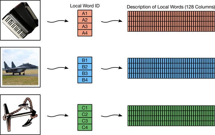
Figure 14.3 Extracting local visual words from the images.
We’ll make use of a few helper functions to locate the image files on our hard drive and to extract the local words from each image.
In [26]:
def img_to_local_words(img):
    ' heavy lifting of creating local visual words from image '
    sift = cv2.xfeatures2d.SIFT_create()
    key_points, descriptors = sift.detectAndCompute(img, None)
    return descriptors

def id_to_path(img_id):
    ' helper to get file location '
    cat, num = img_id
    return osp.join(objcat_path, cat, "image_{:04d}.jpg".format(num))

def add_local_words_for_img(local_ftrs, img_id):
    ' update local_ftrs inplace '
    cat, _ = img_id
    img_path = id_to_path(img_id)
    img = imread(img_path)
    local_ftrs.setdefault(cat, []).append(img_to_local_words(img))
Since processing images can take a lot of time, we’ll restrict ourselves to just a few categories for our discussion. We’ll also set a limit on the number of global vocabulary words we’re willing to create.
In [27]:
# set up a few constants
use_cats = ['accordion', 'airplanes', 'anchor']
use_imgs = range(1,11)

img_ids  = list(it.product(use_cats, use_imgs))
num_imgs = len(img_ids)

global_vocab_size = 20
What do the local visual words look like? Since they are visual words and not written words, they aren’t made up of letters. Instead, they are made up of numbers that summarize interesting regions of the image. Images with more interesting regions have more rows.
In [28]:
# turn each image into a table of local visual words
# (1 table per image, 1 word per row)
local_words = {}
for img_id in img_ids:
    add_local_words_for_img(local_words, img_id)
print(local_words.keys())
dict_keys(['accordion', 'airplanes', 'anchor'])
Over the three categories, we’ve processed the first 10 images (from the use_imgs variable), so we’ve processed 30 images. Here are the numbers of local words for each image:
In [29]:
# itcfi is basically a way to get each individual item from an
# iterator of items; it's a long name, so I abbreviate it
itcfi = it.chain.from_iterable
img_local_word_cts = [lf.shape[0] for lf in itcfi(local_words.values())]
print("num of local words for images:")
print(textwrap.fill(str(img_local_word_cts), width=50))
num of local words for images:
[804, 796, 968, 606, 575, 728, 881, 504, 915, 395,
350, 207, 466, 562, 617, 288, 348, 671, 328, 243,
102, 271, 580, 314, 48, 629, 417, 62, 249, 535]
Let’s try to get a handle on how many local words there are in total.
In [30]:
# how wide are the local word tables
num_local_words = local_words[use_cats[0]][0].shape[1]

# how many local words are there in total?
all_local_words = list(itcfi(local_words.values()))
tot_num_local_words = sum(lw.shape[0] for lw in all_local_words)
print('total num local words:', tot_num_local_words)

# construct joined local tables to perform clustering
# np_array_fromiter is described at the end of the chapter
lwa_shape = (tot_num_local_words, num_local_words)
local_word_arr = np_array_fromiter(itcfi(all_local_words),
                                   lwa_shape)
print('local word tbl:', local_word_arr.shape)
total num local words: 14459
local word tbl: (14459, 128)
We’ve got about 15,000 local visual words. Each local word is made up of 128 numbers. You can think of this as 15,000 words that have 128 letters in each. Yes, it’s weird that all the words have the same length . . . but that’s a limit of our analogy. Life’s hard sometimes.
14.3.3.2 Global Vocabulary and Translation
Now, we need to find out which local visual words are synonyms of each other. We do that by clustering the local visual words together to form the global visual word vocabulary, as in Figure 14.4. Our global vocabulary looks super simple: term 0, term 1, term 2. It’s uninteresting for us—but we are finally down to common descriptions that we can use in our standard classifiers.

Figure 14.4 Creating the global vocabulary.
In [31]:
# cluster (and translate) the local words to global words
translator = cluster.KMeans(n_clusters=global_vocab_size)
global_words = translator.fit_predict(local_word_arr)
print('translated words shape:', global_words.shape)
translated words shape: (14459,)
14.3.3.3 Bags of Global Visual Words and Learning
Now that we have our global vocabulary, we can describe each image as a bag of global visual words, as in Figure 14.5. We just have to morph the global words table and image identifiers into a table of global word counts—effectively, each image is now a single histogram as in Figure 14.6—against the respective image category.
In [32]:
# which image do the local words belong to
# enumerate_outer is descibed at the end of the chapter
which_img = enumerate_outer(all_local_words)
print('which img len:', len(which_img))

# image by global words -> image by histogram
counts = co.Counter(zip(which_img, global_words))
imgs_as_bogvw = np.zeros((num_imgs, global_vocab_size))
for (img, global_word), count in counts.items():
    imgs_as_bogvw[img, global_word] = count
print('shape hist table:', imgs_as_bogvw.shape)
which img len: 14459
shape hist table: (30, 20)

Figure 14.5 Translating local words to the global vocabulary.

Figure 14.6 Collecting global vocabulary counts as histograms.
After all that work, we still need a target: the category that each image came from. Conceptually, this gives us each category of images as the target for a histogram-which-is-our-example (see Figure 14.7).

Figure 14.7 Associating the histograms with a category.
In [33]:
# a bit of a hack; local_ftrs.values() gives
# [[img1, img2], [img3, img4, img5], etc.]
# answers: what category am i from?
img_tgts = enumerate_outer(local_words.values())
print('img tgt values:', img_tgts[:10])
img tgt values: [0 0 0 0 0 0 0 0 0 0]
Finally, we can fit our learning model.
In [34]:
# build learning model
std_svc = pipeline.make_pipeline(skpre.StandardScaler(), svm.SVC())
svc = std_svc.fit(imgs_as_bogvw, img_tgts)
14.3.3.4 Prediction
Now we can recreate the prediction steps we talked about in the overview. We break the prediction steps into two subtasks:
Converting the image on disk into a row-like example in the BoGVW representation
Performing the actual
predictcall on that example
In [35]:
def image_to_example(img_id, translator):
    ' from an id, produce an example with global words '
    img_local  = img_to_local_words(imread(id_to_path(img_id)))
    img_global = translator.predict(img_local)
    img_bogvw  = np.bincount(img_global,
                             minlength=translator.n_clusters)
    return img_bogvw.reshape(1,-1).astype(np.float64)
We’ll check out the predictions from image number 12—an image we didn’t use for training—for each category.
In [36]:
for cat in use_cats:
    test = image_to_example((cat, 12), translator)
    print(svc.predict(test))
[0]
[1]
[2]
We’ll take a closer look at our success rate in a moment.
14.3.4 Complete Code of BoVW Transformer
Now, you can be forgiven if you lost the track while we wandered through that dark forest. To recap, here is the same code but in a streamlined form. Thanks the helper functions—one of which (add_local_words_for_img) is domain-specific for images and others (enumerate_outer and np_array_fromiter) are generic solutions to Python/NumPy problems—it’s just over thirty lines of code to build the learning model. We can wrap that code up in a transformer and put it to use in a pipeline:
In [37]:
class BoVW_XForm:
    def __init__(self):
        pass

    def _to_local_words(self, img_ids):
        # turn each image into table of local visual words (1 word per row)
        local_words = {}
        for img_id in img_ids:
            add_local_words_for_img(local_words, img_id)

        itcfi = it.chain.from_iterable
        all_local_words = list(itcfi(local_words.values()))
        return all_local_words

    def fit(self, img_ids, tgt=None):
        all_local_words = self._to_local_words(img_ids)
        tot_num_local_words = sum(lw.shape[0] for lw in all_local_words)
        local_word_arr = np_array_fromiter(itcfi(all_local_words),
                                           (tot_num_local_words,
                                            num_local_words))
        self.translator = cluster.KMeans(n_clusters=global_vocab_size)
        self.translator.fit(local_word_arr)
        return self

    def transform(self, img_ids, tgt=None):
        all_local_words = self._to_local_words(img_ids)
        tot_num_local_words = sum(lw.shape[0] for lw in all_local_words)
        local_word_arr = np_array_fromiter(itcfi(all_local_words),
                                           (tot_num_local_words,
                                            num_local_words))
        global_words = self.translator.predict(local_word_arr)

        # image by global words -> image by histogram
        which_img = enumerate_outer(all_local_words)
        counts = co.Counter(zip(which_img, global_words))
        imgs_as_bogvw = np.zeros((len(img_ids), global_vocab_size))
        for (img, global_word), count in counts.items():
            imgs_as_bogvw[img, global_word] = count
        return imgs_as_bogvw
Let’s use some different categories with our transformer and up our amount of training data.
In [38]:
use_cats = ['watch', 'umbrella', 'sunflower', 'kangaroo']
use_imgs = range(1,40)

img_ids  = list(it.product(use_cats, use_imgs))
num_imgs = len(img_ids)

# hack
cat_id = {c:i for i,c in enumerate(use_cats)}
img_tgts = [cat_id[ii[0]] for ii in img_ids]
Now, we can build a model from training data.
In [39]:
(train_img, test_img,
 train_tgt, test_tgt) = skms.train_test_split(img_ids, img_tgts)
bovw_pipe = pipeline.make_pipeline(BoVW_XForm(),
                                   skpre.StandardScaler(),
                                   svm.SVC())
bovw_pipe.fit(train_img, train_tgt);
and we just about get the confusion matrix for free:
In [40]:
img_preds = bovw_pipe.predict(test_img)
cm = metrics.confusion_matrix(test_tgt, img_preds)
ax = sns.heatmap(cm, annot=True,
                 xticklabels=use_cats,
                 yticklabels=use_cats,
                 fmt='3d')
ax.set_xlabel('Predicted')
ax.set_ylabel('Actual');

These results aren’t stellar, but we also haven’t tuned the system at all. You’ll have a chance to do that in the exercises. The lesson here is that with a ~30-line transformer, we are well on our way to learning the categories of images.
14.4 EOC
14.4.1 Summary
We’ve taken an even-more-practical-than-usual turn: now we have some tools to work with text and graphics. Along the way, we explored some methods for turning text into learnable features. Then, we saw how to use characteristics of images—in analogy with words—to create learnable features from graphics. Coupled with a new technique called clustering, which we used to gather similar visual words together into a common visual vocabulary, we were able to classify images.
14.4.2 Notes
If you’d like to see the exact stop words used by sklearn, go to the sklearn source code (for example, on github) and find the following file: sklearn/feature_extraction/stop_words.py.
If we cluster over all of the features, we will get a single group (one cluster label) for each example—a single categorical value. You could consider performing clustering on different subsets of features. Then, we might get out several new quasi-columns containing our clusters with respect to the different subsets. Conceptually, using a few of these columns—several different views of data—might get us better predictive power in a learning problem.
Helpers There are two quick utilities we made use of in our bag-of-visual-words system. The first is similar to Python’s built-in enumerate which augments the elements of a Python iterable with their numeric indices. Our enumerate_outer takes an iterable of sequences—things with lengths—and adds numeric labels indicating the position in the outer sequence that the inner element came from. The second helper takes us from an iterable of example-like things with the same number of features to an np.array of those rows. numpy has a built-in np.fromiter but that only works when the output is a single conceptual column.
In [41]:
def enumerate_outer(outer_seq):
    '''repeat the outer idx based on len of inner'''
    return np.repeat(*zip(*enumerate(map(len, outer_seq))))

def np_array_fromiter(itr, shape, dtype=np.float64):
    ''' helper since np.fromiter only does 1D'''
    arr = np.empty(shape, dtype=dtype)
    for idx, itm in enumerate(itr):
        arr[idx] = itm
    return arr
Here are some quick examples of using these helpers:
In [42]:
enumerate_outer([[0, 1], [10, 20, 30], [100, 200]])
Out[42]:
array([0, 0, 1, 1, 1, 2, 2])
In [43]:
np_array_fromiter(enumerate(range(0,50,10)), (5,2))
Out[43]:
array([[ 0.,  0.],
       [ 1., 10.],
       [ 2., 20.],
       [ 3., 30.],
       [ 4., 40.]])
14.4.3 Exercises
Conceptually, we could normalize—with
skpre.Normalizer—immediately once we have document word counts, or we could normalize after we compute the TF-IDF values. Do both make sense? Try both methods and look at the results. Do some research and figure out which methodTfidfVectorizeruses. Hint: use the source, Luke.In the newsgroups example, we used
TfidfVectorizer. Behind the scenes, the vectorizer is quite clever: it uses a sparse format to save memory. Since we built a pipeline, the documents have to flow through the vectorizer every time we remodel. That seems very time-consuming. Compare the amount of time it takes to do 10-fold cross-validation with a pipeline that includesTfidfVectorizerversus performing a singleTfidfVectorizerstep with the input data and then performing 10-fold cross-validation on that transformed data. Are there any dangers in “factoring out” theTfidfVectorizerstep?Build models for all pairwise newsgroups classification problems. What two groups are the most difficult to tell apart? Phrased differently, what two groups have the lowest (worst) classification metrics when paired off one-versus-one?
We clustered the iris dataset by first preprocessing with PCA. It turns out that we can also preprocess it by using
discriminant_analysis.LinearDiscriminantAnalysis(LDA) with an_componentsparameter. From a certain perspective, this gives us a class-aware version of PCA: instead of minimizing the variance over the whole dataset, we minimize the variance between classes. Try it! Usediscriminant_analysis.LinearDiscriminantAnalysisto create two good features for iris and then cluster the result. Compare with the PCA clusters.We used a single, fixed global vocabulary size in our image classification system. What are the effects of different global vocabulary size on learning performance and on resource usage?
We evaluated our image classification system using a confusion matrix. Extend that evaluation to include an ROC curve and a PRC.
In the image system, does using more categories help with overall performance? What about performance on individual categories? For example, if we train with 10 or 20 categories, does our performance on kangaroos increase?