Chapter 2. Contouring and Contouring Techniques*
* For all figures in this chapter (in the printed book only), see the preface for information about registering your copy on the InformIT site for access to the electronic versions in color.
Introduction
A wide variety of subsurface maps are discussed in the following chapters. Each map presents a specific type of subsurface data obtained from one or more sources. The purposes of these maps are to present data in a form that can be understood and used to explore for, develop, or evaluate energy resources such as oil and gas.
It might seem elementary to have a chapter on contouring, since most geologists are taught the basics of contouring in several introductory geology courses. However, there are two good reasons for this chapter. First, part of our audience includes members of the geophysical and petroleum engineering disciplines. They may have had little, if any, training in basic contouring principles and methods. Second, because the understanding and correct application of contouring and contouring techniques is of paramount importance in establishing a solid foundation in subsurface mapping, a review of contouring is appropriate.
The majority of subsurface maps use the contour line as the vehicle to convey the various types of subsurface data. By definition, a contour line is a line that connects points of equal value. Usually this value is compared to some chosen reference, such as sea level in the case of structure contour maps. In preparing subsurface maps, we are dealing with data beneath the earth’s surface, which cannot be seen or touched directly. Therefore, the preparation of a geologically reasonable subsurface map requires an in-depth knowledge of geology, interpretation skills, imagination, an understanding of 3D geometry, and the use of correct mapping techniques.
Any map that uses the contour line as its vehicle for illustration is called a contour map. A contour map illustrates a 3D surface or solid in 2D plan (map) view. Any set of data that can be expressed numerically can be contoured.
The following list shows examples of contourable data and the associated contour map.
Data |
Type of Map |
|---|---|
Elevation |
Structure, Fault, Salt |
Thickness of sediments |
Interval Isopach |
Percentage of sand |
Percent Sand |
Feet or meters of pay |
Net Pay Isochore |
Pressure |
Isobar |
Temperature |
Isotherm |
Time |
Isochron |
Lithology |
Isolith |
If the same set of data points to be contoured is given to several interpreters, the individually contoured maps generated would likely be different. Differences in an interpretation are the result of educational background, the amount of geological training, field and work experience, imagination, and interpretive abilities (such as visualizing in three dimensions). Yet the use of all the available data and an understanding and application of the basic principles and techniques of contouring should be the same. These principles and actual techniques are fundamental to the construction of a mechanically correct map.
In the first part of this chapter, the importance of visualizing in three dimensions and the basic rules of contouring are discussed. In addition, various techniques for contouring by hand are illustrated and certain important guidelines identified. Later, computer-based contouring is discussed.
Three-Dimensional Perspective
In this section, we show how 3D surfaces are represented by contours in map view. A good understanding of the geometry within our subsurface geological world, tectonics, and the principles of 3D spatial relationships are essential to any attempt at constructing a picture of the subsurface. Some geoscientists have a stronger educational background in the geological sciences than others. In addition, some geoscientists have an innate ability to visualize in three dimensions, whereas others do not. One of the best ways to develop this ability is to practice perceiving objects in three dimensions.
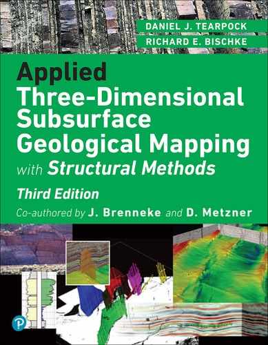
In its simplest form, we can view a plane dipping in the subsurface with respect to the horizontal. (The reference datum for all the examples shown is sea level.) Figure 2-1 shows an isometric view of a plane dipping at an angle of 45 deg with respect to the horizontal and a projection of that dipping plane upward onto a horizontal surface to form a contour map. This dipping plane intersects an infinite number of horizontal planes; but, for any contour map, only a finite set of evenly spaced horizontal plane intersections can be used to construct the map. (For a subsurface structure contour map, the intersections used may be 50 ft or m, 100 ft or m, or even 500 ft or m apart.) By choosing evenly spaced finite values, we have established the contour interval for the map.
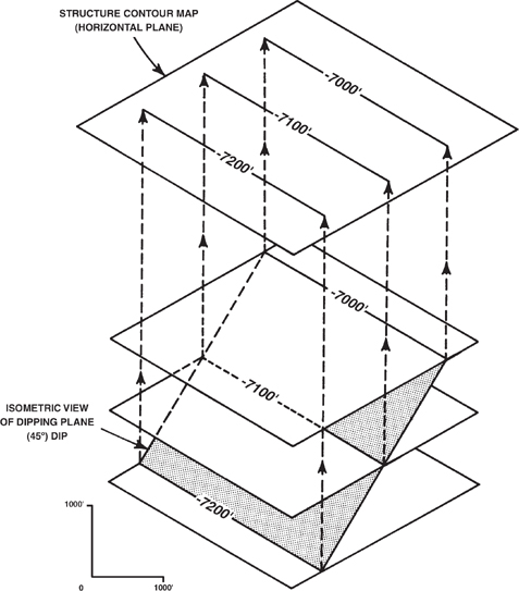
Figure 2-1 Isometric view of dipping plane intersecting three horizontal planes. (Modified from Appelbaum. Geological & Engineering Mapping of Subsurface: A workshop course by Robert Appelbaum. Published by permission of Pearson Education, Inc.)
Next, it is important to choose values that are easy to use for the contour lines. For example, if a 100-ft contour interval is chosen, then the contour line values selected to construct the map should be in even increments of 100 ft, such as 7000 ft, 7100 ft, and 7200 ft. Any increment of 100 ft could be chosen, such as 7040 ft, 7140 ft, and 7240 ft. This approach, however, makes the map more difficult to construct and harder to read and understand. In Figure 2-1, a 100-ft contour interval was chosen for the map (the minus sign in front of the depth value indicates the value is below sea level). The intersection of each horizontal plane with the dipping plane results in a line of intersection projected into map view on the contour map above the isometric view. This contour map is a 2D representation of the 3D dipping plane.
Now we complicate the picture by introducing a dipping surface that is not a plane but is curved (Fig. 2-2). The curved surface intersects an infinite number of horizontal planes, as did the plane in the first example. Each intersection of two surfaces results in a line of intersection, which everywhere has the same value. By projecting these lines into plan view onto a contour map, a 3D surface is represented in two dimensions. If we consider the curved surface as a surface with a changing slope, then the spacing of the contours on the map is representative of the change in slope of the curved surface. In other words, steep slopes are represented by closely spaced contours, and gentle slopes are represented by widely spaced contours (Figs. 2-2 and 2-3). This relationship of contour spacing to change in slope angle assumes that the contour interval for the map is constant.

Figure 2-2 Isometric view of a curved surface intersecting a finite number of evenly spaced horizontal planes. (Modified from Appelbaum. Geological & Engineering Mapping of Subsurface: A workshop course by Robert Appelbaum. Published by permission of Pearson Education, Inc.)

Figure 2-3 The spacing of contour lines is a function of the shape and slope of the surface being contoured.
Finally, we must emphasize that any person generating a subsurface map must have the geological background to understand whether or not the map produced truly represents what is possible in the subsurface. Too often, contour maps violate geological principles or depict structures that are unlikely or even impossible in the subsurface. All maps generated, whether done by hand or computer, must be driven by sound geological principles. Computers are fast, but the accuracy of the resultant interpretation or map is dependent on many factors, such as the algorithm used for gridding, distribution of data, and other factors (refer to section Computer-Based Contouring Concepts and Applications). The computer is a tool, as are an engineer’s scale and ten-point spacing dividers. Yes, it is a powerful tool, but nonetheless a tool. We cannot accept computers driving interpretations, nor can we blindly accept the resultant maps. Our educational background, experience, and geological principles should control any interpretation or generated map. The workstations and personal computers in wide usage today are powerful, but they are not artificial intelligence capable of generating geologically and geometrically reasonable interpretations or maps.
Look at a 3D subsurface formation that is similar in shape to a topographic elongated anticline and the contour map representing that surface (Fig. 2-4). The contour map graphically illustrates the subsurface formation in the same manner that a topographic map depicts the surface of the earth. By using your ability to think in three dimensions, it is possible to look at the contour map and visualize the formation in its true subsurface 3D form.
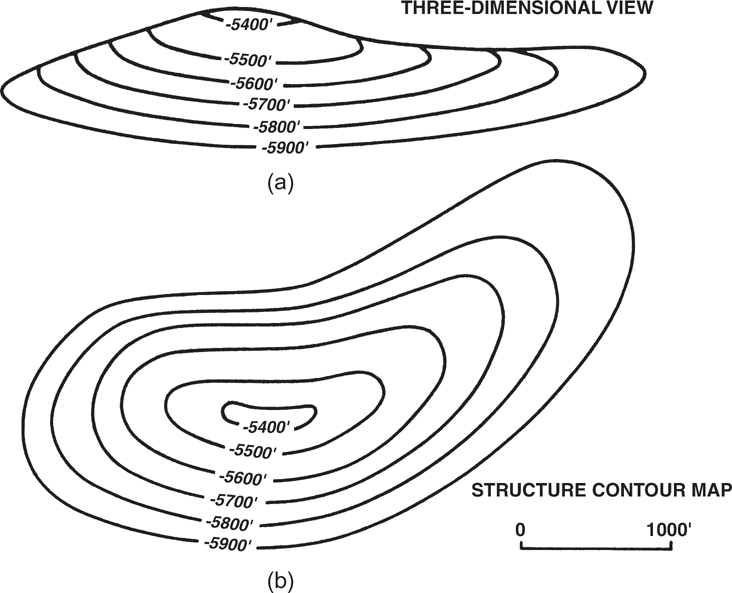
Figure 2-4 (a) A 3D view of an anticlinal structure and (b) the contour map representing the structure.
Calculation of Bed Dip
Contour spacing not only provides a qualitative measure of bed dip, with closely spaced contours representing steeply dipping surfaces and widely spaced contours representing gently dipping surfaces, it also allows for the quantitative calculation of bed dip. The contour interval measures the elevation change on a surface. The contour spacing, measured from the scale of the map, reflects the horizontal distance over which the depth of the surface changes by the contour interval. The elevation change determined from the contour interval is typically called the rise, and the contour spacing is called the run. From basic trigonometry,
where

Rearranging,

where

To get true bed dip, the contour spacing must be measured perpendicular to the strike of the contours. Contour spacing measured at any other angle will yield an apparent dip that is less than the true dip. A graph of apparent dip and the angle between the line of section and the true dip direction is presented in Suppe (1985).
The preceding discussion applies to depth structure maps. Bed dip can be determined qualitatively from contour spacing on time structure maps. Bed dip cannot be calculated quantitatively from time structure (isochron) maps without converting the time contours into depth. The depth interval between time contours is frequently not constant over the area of a structure map, as interval velocity is generally a function of depth and may also vary laterally.
Rules of Contouring
Several rules must be followed in order to draw mechanically correct contour maps. This section lists these rules and discusses a few exceptions.
A contour line cannot cross itself or any other contour except under special circumstances (see rule 2). Since a contour line connects points of equal value, it cannot cross a line of the same value or lines of different values.
A contour line cannot merge with contours of the same value or different values. Contour lines may appear to merge or even cross where there is an overhang, overturned fold, or vertical surface (Fig. 2-5). With these exceptions, the key word is appear. Consider a vertical cliff that is being mapped. In map view the contours appear to merge, but in 3D space these lines are above each other. For the sake of clarity, contours should be dashed on the underside of an overhang or overturned fold.
Figure 2-5 To clearly illustrate a 3D overhang or overturned fold, dash the contours on the underside of the structure. (From Tearpock and Harris 1987. Published by permission of Tenneco Oil Company.)
A contour line must pass between points whose values are lower and higher than its own value (Fig. 2-6). In other words, there must be a contour line between points whose values are lower and higher than the value of the contour line.
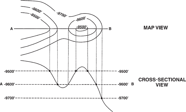
Figure 2-6 A contour line must be repeated to show reversal of slope direction. (From Tearpock and Harris 1987. Published by permission of Tenneco Oil Company.)
A contour line of a given value is repeated to indicate reversal of slope direction. Figure 2-6 illustrates the application of this rule across a structural high (anticline) and a structural low (syncline).
A contour line on a continuous surface must close within the mapped area or end at the edge of the map. Geoscientists often finesse this rule by preparing what is commonly referred to as a postage stamp map. This is a map that covers a very small area when compared to the areal extent of the structure. It is very easy to close a contour line at the edge of a postage stamp map.
These five contouring rules are simple. If they are followed during mapping, the result will be a map that is mechanically correct. Some computer mapping software may be programmed to obey these five rules, but not all mapping software is so programmed. In addition to these rules are other guidelines to contouring that make a map easier to construct, read, and understand.
All contour maps should have a chosen reference to which the contour values are compared. A structure contour map, as an example, typically uses mean sea level as the chosen reference. Therefore, the elevations on the map can be referenced as being above or below mean sea level. A negative sign in front of a depth value means the elevation is below sea level (e.g., −7000 ft).
The contour interval on a map should be constant. The use of a constant contour interval makes a map easier to read and visualize in three dimensions because the distance between successive contour lines has a direct relationship to the steepness of slope. Remember, steep slopes are represented by closely spaced contours and gentle slopes by widely spaced contours (see Fig. 2-3). If for some reason the contour interval is changed on a map, it should be clearly indicated. This can occur where a mapped surface contains both very steep and gentle slopes, such as those seen in areas of salt diapirs. The choice of a contour interval is an important decision. Several factors must be considered in making such a choice. These factors include the density of data, the practical limits of data accuracy (e.g., directional surveys), the steepness of slope, the scale of the map, and its purpose. If the contour interval chosen is too large, small closures with less relief than the contour interval may be overlooked. If the contour interval is too small, however, the map can become too cluttered and reflect inaccuracies of the basic data.
All maps should include a graphic scale (Fig. 2-7). Many people may eventually work with or review a map. A graphic scale provides an exact reference and gives the reviewer an idea of the areal extent of the map and the magnitude of the features shown. Also, it is not uncommon for a map to be reproduced, projected, or viewed on a computer screen. During this process, the map may be reduced or enlarged. Without a graphic scale, the values shown on the map may become useless. Because it is easy to stretch or squeeze a map on a computer, we recommend that scale bars have both an X and a Y graphic scale (Fig. 2-7).
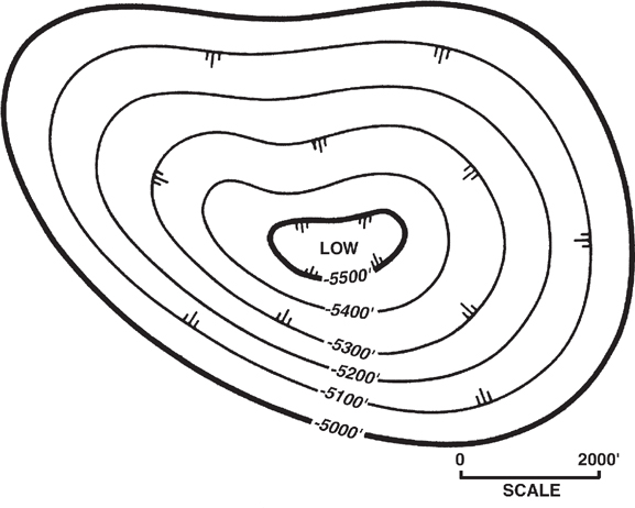
Figure 2-7 Closed depressions are indicated by hachured lines.
Every fifth contour should be thicker than the other contours, and it should be labeled with the value of the contour. This fifth contour is referred to as an index contour. For example, with a structure contour map using a 100-ft contour interval, it is customary to thicken and label the contours every 500 ft. At times it may be necessary to label other contours for clarity (Fig. 2-7).
Hachured lines should be used to indicate closed depressions (Fig. 2-7).
Start contouring in areas with the maximum number of control points (Fig. 2-8).
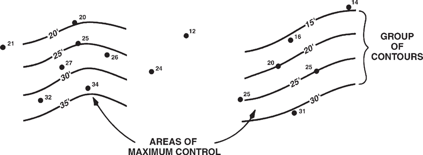
Figure 2-8 Begin contouring in areas of maximum control using groups of contour lines.
Construct the contours in groups of several lines rather than one single contour at a time (Fig. 2-8). This should save time and provide better visualization of the surface being contoured.
Initially, choose the simplest contour solution that honors the control points and provides a realistic subsurface interpretation.
Use a smooth rather than undulating style of contouring unless the data indicate otherwise (Fig. 2-9).

Figure 2-9 A smooth style of contouring is preferred over an undulating style.
Initially, a hand-drawn map should be contoured in pencil with the lines lightly drawn so they can be erased as the map requires revision.
If possible, prepare hand-contoured maps on some type of transparent material such as mylar or vellum. Often, several individual maps have to be overlaid one on top of the other (see Chapter 8). The use of transparent material makes this type of work easier and faster.
Methods of Contouring by Hand
As mentioned previously, different contoured interpretations can be constructed from the same set of values. The differences in the finished maps may be the result of the geoscientists’ educational background, experience levels, interpretive abilities, or other individual factors. This section establishes that the differences can also be the result of the method of contouring used by each geoscientist (see section Computer-Based Contouring).
Unlike topographic data, which are usually obtainable in whatever quantity needed to construct very accurate contour maps, data from the subsurface is scarce. Therefore, any subsurface map is subject to individual interpretation. The amount of data, the areal extent of that data, and the purpose for which a map is being prepared may dictate the use of a specific method of contouring. There are four distinct methods of hand contouring: (l) mechanical, (2) equal-spaced, (3) parallel, and (4) interpretive (Rettger 1929; Bishop 1960; and Dennison 1968).
Mechanical Contouring. By using this method of contouring, one may assume that the slope or angle of dip of the surface being contoured is uniform between points of control and that any change occurs at the control points. Figure 2-10 is an example of a mechanically contoured map. With this approach, the spacing of the contours is mathematically (mechanically) proportioned between adjacent control points. We use line A-A' in Figures 2-10 and 2-11 to illustrate this method of contouring. Wells No. 2, 4, and 5 lie on line A-A' with depths of 600 ft, 400 ft, and 200 ft, respectively. The contour interval used for this map is 100 ft. First, we can see that the 600-ft, 400-ft, and 200-ft contour lines pass through Wells No. 2, 4, and 5. Next, we need to determine the position of the 500-ft and 300-ft contour lines. Remembering that this method assumes a uniform slope or dip between control points, we can use ten-point spacing dividers or an engineer’s scale to interpolate the location of these two contour lines. The 500-ft contour line lies midway between the 600-ft and 400-ft contour lines. Likewise, the 300-ft contour line is placed midway between the 400-ft and 200-ft contour lines. When this procedure is repeated for all adjacent control points, the result is a mechanically contoured map that is geometrically accurate.
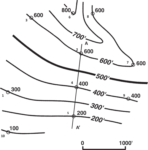
Figure 2-10 Mechanical contouring method. (Modified from Bishop 1960. Published by permission of author.)
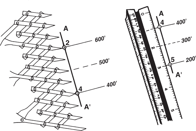
Figure 2-11 Two different methods of establishing contour spacing.
Mechanical contouring allows for little, if any, geological interpretation. Even though the map is mechanically correct, the result may be a map that is geologically unreasonable, especially in areas of sparse control.
Although mechanical contouring is not recommended for most contour mapping, it does have application in a few areas and may be a good first step when beginning work in a new geographic area. When there is a sufficient amount of seismic or well control, such as in a densely drilled mature oil or gas field, this method may provide reasonable results, since there is little room for interpretation. This method is at times employed in litigation, equity determinations, and unitization because it supposedly minimizes individual bias in the contouring. However, although individual bias may be minimized, the method does not allow for true geological interpretation. The method is therefore not recommended for the activities listed here.
2. Parallel Contouring. With this method of contouring, the contour lines are drawn parallel or nearly parallel to each other. This method does not assume uniformity of slope or angle of dip as in the mechanical contouring method. Therefore, the spacing between contours may vary (Fig. 2-12).

Figure 2-12 Parallel contouring method. (Modified from Bishop 1960. Published by permission of author.)
As with the previous method, if honored exactly, parallel contouring may yield an unrealistic geological picture. Figure 2-13 shows a map that has been contoured using this method. Notice that the highs appear as bubble-shaped structures with the adjoining synclines represented as sharp cusps. This map depicts an unreasonable geological picture.
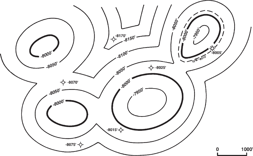
Figure 2-13 An example of an unrealistic structure map constructed using the parallel contouring method.
Although this method may yield an unrealistic map, it does have advantages over mechanical contouring. First, the method allows some geological license to draw a more realistic map than one constructed using the mechanical method, because there is no assumption of uniform dip between control points. Also, this method is not as conservative as true mechanical contouring. Therefore, it may reveal features that would not be represented on a mechanically contoured map.
Parallel contouring is frequently used for fault surface maps (e.g., Figs. 7-12 and 7-47) where the dip of the fault may change with depth but the strike of the fault is relatively constant with depth.
3. Equal-Spaced Contouring. This method of contouring assumes uniform slope or angle of dip over an entire area, over an individual flank, or over a segment of a structure. Sometimes this method is referred to as a special version of parallel contouring. Equal-spaced contouring is the least conservative of the three methods discussed so far.
To use this method, choose closely spaced data and determine the slope or angle of dip between them. Usually the slope or angle of dip chosen for mapping is the steepest found between adjacent control points. Once the dip is established, it is held constant over the entire mapped area. In the example shown in Figure 2-14, the dip rate between Wells No. 2 and 4 was used to establish the rate of dip for the entire map.

Figure 2-14 Equal-spaced contouring method. (Modified from Bishop 1960. Published by permission of author.)
Since the equal-spaced method of contouring is the least conservative, it may result in numerous highs, lows, or undulations that are not based on established points of control but are the result of maintaining a constant dip rate or slope. The advantage to this method, in the early stages of mapping, is that it may indicate a maximum number of structural highs and lows expected in the study area. One assumption that must be made in using this method is that the data used to establish the slope or rate of dip are not on opposite sides of a nose or on opposite flanks of a fold. In Figure 2-14, Wells No. 6 and 8 are on the northern flank of this structure; therefore, neither well can be used with a well on the southern flank to establish the rate of dip. These two wells can be and were used to establish the rate of dip for contouring the northern flank of this southeast trending structural nose.
This method does have application on the flanks of structures that have a uniform dip, such as kink band folds. For example, the back limb of a fault bend fold, which typically is parallel to the dip of the thrust fault that formed the fold, may have a constant dip between axial surfaces (Fig. 10-36). In such a case, the equal-spaced method of contouring may have some applicability in contouring this back limb.
4. Interpretive Contouring. With this method of contouring, a geoscientist has extreme geological license to prepare a map to reflect the best interpretation of the area of study while honoring the available control points (Fig. 2-15). No assumptions, such as constant bed dip or parallelism of contours, are made when using this method. Therefore, the geoscientist can use experience, imagination, ability to think in three dimensions, and an understanding of the structural and depositional style in the geological region being worked to develop a realistic interpretation. Interpretive contouring is the most acceptable and the most commonly used method of hand contouring.
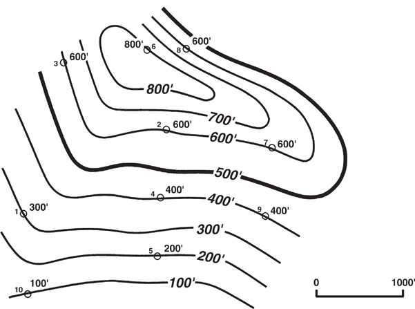
Figure 2-15 Interpretive contouring method. (Modified from Bishop 1960. Published by permission of author.)
As mentioned earlier, the specific method chosen for contouring may be dictated by such factors as the number of control points, the areal extent of these points, and the purpose of the map. It is essential to remember that no matter which method is used in making a subsurface map, the map is not correct. No one can really develop a correct interpretation of the subsurface with the same accuracy as that of a topographic map. What is important is to develop the most reasonable and realistic interpretation of the subsurface with the available data, whether the maps are constructed by hand or with the use of a computer.
As an exercise in contouring methods, use vellum to contour the data points in Figure 2-16, using all four methods, and compare the results. Which method results in the most optimistic picture? The most pessimistic?
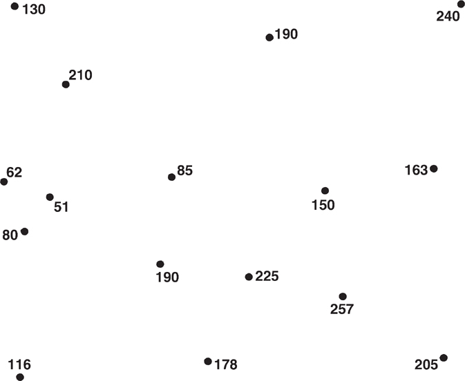
Figure 2-16 Data points to be contoured using all four methods of contouring. (Reproduced from Analysis of Geologic Structures by John M. Dennison, by permission of W. W. Norton & Company, Inc. Copyright 1968 by W. W. Norton & Company, Inc.)
Special guidelines are used in contouring fault, structure, and isochore maps. Additional guidelines for these maps are discussed in the appropriate chapters. When using computers for mapping, there are other guidelines that should be used or at least considered.
Computer-Based Contouring Concepts and Applications
Computers have altered the way we make geological and geophysical maps. They allow us to quickly create a map without having to think about the surface that is being contoured. They give us the ability to generate a map to the point where the actual geology may be overlooked. Computers have made it easy to skip tried-and-tested techniques that ensure accurate maps because those techniques take too long or are not available in the computer program. This is the downside of computer mapping, the side that lacks the interpretive chemistry that occurs when a geoscientist draws contours by hand and thinks about a surface being contoured. That interpretive thought process in many instances has been replaced with concerns about transferring data from one program to another and learning which parameters will actually create a surface map. There is an upside to computer mapping, as well. With the speed and power of computers, the geoscientist can quickly test many interpretations, easily check two surfaces to see whether they cross, use colors to see whether faults reverse direction along strike, and view in three dimensions the created surface to understand the reasonableness and validity of its form. With computers, just as with hand contouring, if the correct methods and proper quality control are not used, then the generated map will likely be wrong.
In this section we discuss how the concepts used in contouring by hand may be implemented on a computer. What is simple for the human brain to accomplish may be extremely difficult for the computer. The contouring we discuss is limited to data sets where we do not have an unlimited number of data points, as would be available for topographic data. Instead, we cover computer contouring of data that represents a surface that has been “sampled” at a limited number of locations (e.g., wells, seismic bins, gravity or magnetic stations). We do not have a precise mathematical equation for the surface, nor do we have aerial photographs. This process of contouring is sometimes called surface modeling.
Surface Modeling
We start from a table of X, Y, and Z, where X and Y define the locations of our samples and Z is the height of the surface at that location. The problem is to position the contour lines so as to depict a reasonable geological surface. Mathematically, this is an interpolation problem.
It can be said that interpolation is the mathematical art of estimating. An interpolation process calculates the value (height) of a surface at locations where it is unknown, based on the values at locations where it is known. Interpolation is an art in the sense that there is no limit to the number of mathematical formulae that may be conceived to make the estimates, and the choice of formulae includes subjective and aesthetic criteria: Does the map look geologically reasonable? Does it come close to how you would do it by hand? Is it pleasing?
The great mathematicians of the past, Newton, Sterling, Chebyshev, Gauss, among others, who dealt with interpolation methods, did not address (or at least did not publish) satisfactory methods to deal with 3D, randomly distributed data. This fact, plus the subjective and aesthetic requirements of contour maps, explains the proliferation of computer contouring methods that have evolved in the past few decades. Two approaches to deal with random data distribution have emerged: indirect (gridded) and direct (nongridded).
Indirect Technique (Gridding).
Computer contouring methods that use the gridding technique typically start by using the primary (original) data points to generate a set of secondary (calculated) points. These secondary points, which are traditionally along an orderly geometric pattern (grid), then replace the primary data in steps that generate the contour maps. All subsequent calculations to locate the positions of the contour lines use the secondary data set (the grid). The purpose of using this technique is to simplify the subsequent steps by making the geometry more manageable.
It is easy to ensure that any contour line drawn through a data grid honors its given grid of data points. However, contour lines that honor the data grid cannot be guaranteed to honor the original (primary) data points.
Direct Technique (Triangulation).
The triangulation technique is the most common of the direct contouring techniques that interpolate values along a pattern which need not be regular but which is derived from the pattern of the original data. The pattern includes the locations of the original data, which are kept throughout the subsequent processing, thus providing the opportunity that all contour lines will honor all the original data.
For both techniques, gridding and triangulation, many ways exist to solve the basic problem. Our goal is to choose a technique that most nearly fulfills the needs of the user: geologist, geophysicist, or engineer. In general, the computer-contoured map is more acceptable to the user if it is geologically reasonable and looks as if it has been contoured by hand.
Steps Involved in Gridding
Gridding has come to mean using the original data points to estimate values at the calculated points, or grid nodes. Gridding always involves three steps:
Select a grid size and origin.
Select neighboring data points to be used in calculating a value at each grid node.
Estimate the value at that grid node using values from the neighboring points.
The last two steps are where numerous schemes have been developed to make maps that are aesthetically pleasing and that honor the data points as much as possible.
Selecting Neighbors and Estimating Values at Grid Nodes. We now describe some of the methods used for selecting neighbors and estimating values at grid nodes. When selecting neighbors, two criteria are important: (1) neighbors should be evenly distributed around the grid node, and (2) only data points near the grid node should be considered neighbors. As we discuss some of the methods for selecting neighbors, certain data distributions will make it difficult to meet these criteria. We now describe several (out of many) schemes to select neighbors.
Nearest “n” Neighbors. This is the simplest method of selecting neighbors (Fig. 2-17a). Although this method gives acceptable results for evenly distributed data, it has problems when applied to an uneven data set. For example, where data have been gathered along a straight line (e.g., 2D seismic data, as in Fig. 2-17b), all data points may lie on one side of the grid node. Linear data are unsuitable for surface fitting. To ensure that data are chosen on all sides of a grid node, the domain around the node may be broken into sectors, or segments, such as quadrant, octant, or other pie segments. One method of ensuring a better distribution of data around each grid node is by sector search. Eight sectors are used in Figure 2-18. In the sector search, a certain number, “n,” of nearest neighbors are selected from each segment. Obviously, the neighborhood has to expand in order to find some neighbors in each segment. This may mean ignoring some nearby control points in order to satisfy the limitation that only “n” points be taken from each segment.

Figure 2-17 (a) “n” nearest neighbors. This is the simplest method of selecting neighbors. (b) “n” nearest neighbors may all be on one side of grid node for 2D seismic data. (AAPG©1991, reprinted by permission of the AAPG whose permission is required for further use.)
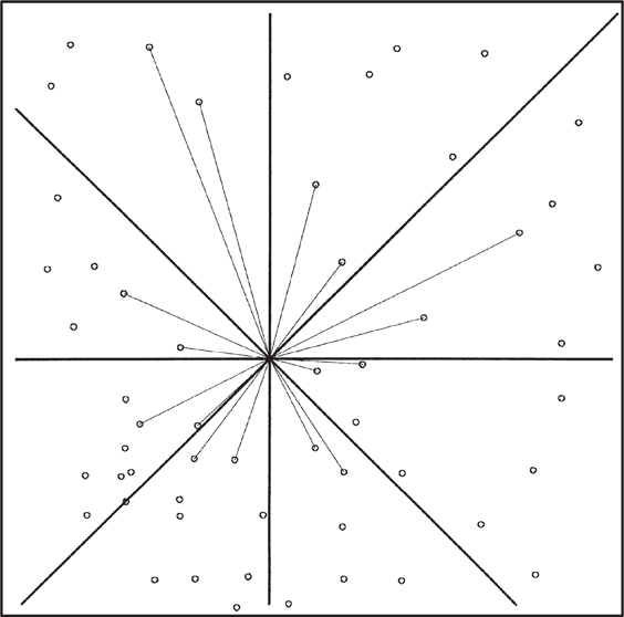
Figure 2-18 Two nearest neighbors in each octant. (AAPG©1991, reprinted by permission of the AAPG whose permission is required for further use.)
One obvious drawback to any of the sector search procedures is their lack of uniqueness; that is, if the data are rotated, neighbors and neighborhoods change. It would be preferable to find a method that is invariant under rotation.
2. Natural Neighbors. On a flat surface that contains more than two data points, any three data points that lie on the circumference of a circle that contains no other data points form what is called a Delaunay triangle. These three points are also defined as natural neighbors.
Estimating Values at Grid Nodes.
Once we have selected neighbors of a grid node, we proceed to use the Z values of these neighbors to estimate a value (and perhaps a slope) at the grid node. The following are some of the methods used:
1. |
Weighted average |
6. |
Minimum curvature |
2. |
Least squares |
7. |
Polynomial fit |
3. |
Tangential |
8. |
Double Fourier |
4. |
Spline |
9. |
Triangle plane |
5. |
Hyperbolic |
Each of these methods (and other schemes) has its advocates and adversaries. Any of them works well if the data points are well distributed and well behaved. Each method has problems under certain circumstances.
Most gridded contouring programs give their users an opportunity to select the method of choosing neighbors and the method for estimating values at grid nodes. All gridded contouring programs require users to select grid size.
The pertinent points about indirect techniques (gridding) are:
Gridding can never guarantee maps that honor all of the data points. On the other hand, the nonhonoring of data may be acceptable if the data are noisy or if the calculated value and the observed value at a data point location differ by an amount that is within the accuracy of the data. In fact, if the data are particularly noisy, the maps may be more pleasing if all of the data are not honored.
Sparse data sets that contain clusters of closely spaced data can be troublesome for computer contouring systems, gridded or nongridded. An example of such clustered data distribution is in oil and gas exploration areas, which include wildcat areas (sparse data) and some oil and gas fields (clustered data).
Changing the grid size often produces a different map because the neighbors of grid nodes change with changes in grid size.
The user must choose a method of selecting neighbors and a method of estimating values at grid nodes (interpolation).
Steps Involved in Triangulation.
Triangulation in contouring is almost instinctive. Most of us, consciously or subconsciously, were triangulating when we were learning to contour in college. We connected data points with straight lines and subdivided the lines according to contour intervals. At the end of the process, the straight lines connecting the data points were a fairly good approximation of Delaunay triangles. It is therefore not surprising that triangulation, which involves subdividing the map area into triangles (leaving no gaps and creating no overlap), was one of the earlier proposed first steps toward computer contouring.
As in gridding, triangulation requires the selection of neighbors for each data point. However, in triangulation the task of determining neighbors is finished when the data set has been triangulated. The resulting triangulation has the following characteristics:
The X-Y data set containing “n” data points has been broken down into a set of (2n-m-2) triangles, where “m” is the number of data points on the convex hull. The convex hull is defined as the smallest convex polygon that encloses all of the data.
If the triangles are Delaunay triangles, they are as nearly equilateral as possible for any data distribution, and they are invariant under rotation.
In large data sets, each data point will have an average of six natural neighbors.
Figure 2-19 is a sample data set with Delaunay triangles connecting natural neighbors. If no interpolation were performed, and if the surface being contoured were treated as flat in each triangle, the map would have the characteristics of mechanical contouring and would look like Figure 2-20.
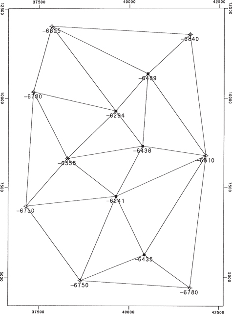
Figure 2-19 Delaunay triangles and natural neighbors. (AAPG©1991, reprinted by permission of the AAPG whose permission is required for further use.)
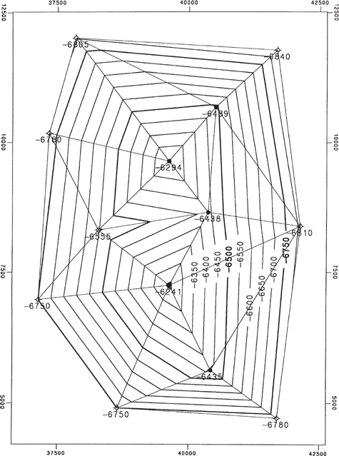
Figure 2-20 Mechanical contouring in basic Delaunay triangles. (Published by permission of Scientific Computer Applications, Inc.)
Mechanical contouring, however, tends to be very angular and unrealistic. It is usually necessary to interpolate values within the Delaunay triangles (i.e., create more and smaller triangles) based on curved mathematical models in order to overcome the angular appearance. Figure 2-21 shows a set of the subtriangles formed when each leg of the original Delaunay triangles is divided into 16 segments.
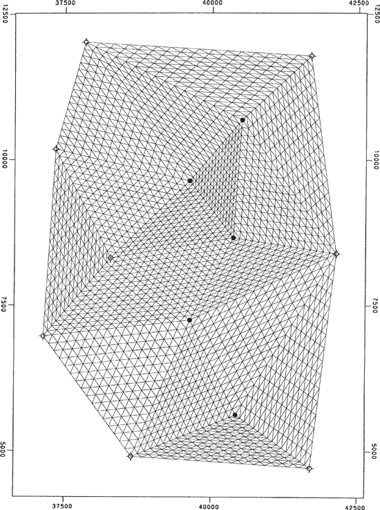
Figure 2-21 Subtriangles forming each side of Delaunay triangles are divided into 16 segments. (AAPG©1991, reprinted by permission of the AAPG whose permission is required for further use.)
The pertinent points about triangulation are:
Triangulation always honors every data point because the original data points always remain in the data set being contoured.
The interpretation is essentially the same, regardless of the number of triangles or smoothing.
The user does not have to worry about data distribution.
Sample Data Set.
Figure 2-22 shows a small (13-point) data set representing a structural surface. We encourage you to contour these data yourself before reviewing the computer-contoured maps. These were the data used to generate Figures 2-19, 2-20, and 2-21. Figures 2-23a through f are montages of contour maps of these data generated using various gridded contouring programs, which in turn used various methods of (1) selecting neighbors and (2) calculating values at grid nodes. Figure 2-24 is a contour map of these same data generated using Delaunay triangles, where a value was interpolated at each vertex of the subtriangles shown in Figure 2-21.
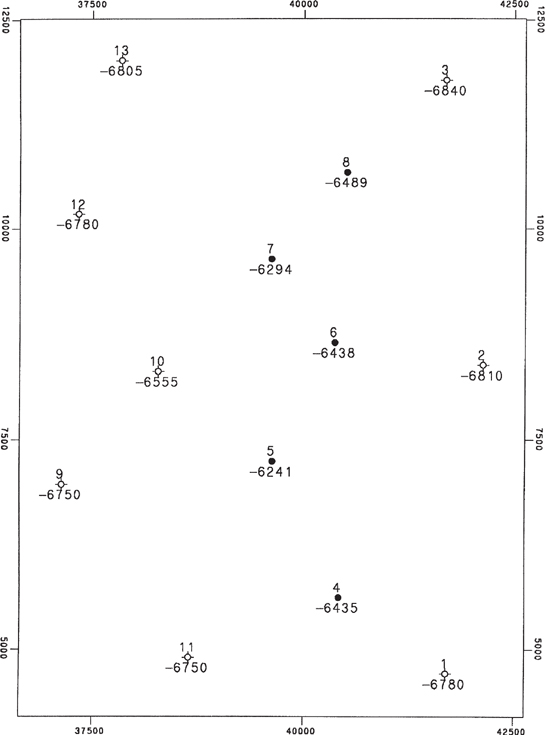
Figure 2-22 Sample data set. (AAPG©1991, reprinted by permission of the AAPG whose permission is required for further use.)

Figure 2-23 (a)–(f) Six structural contour maps using various gridding methods for the same data set. (Published by permission of Scientific Computer Applications, Inc.)
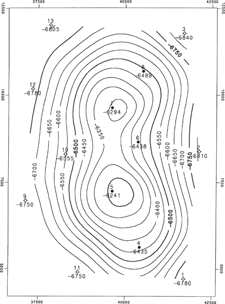
Figure 2-24 Contour map of sample data generated using subtriangles of Delaunay triangles as illustrated in Figure 2-21. (AAPG©1991, reprinted by permission of the AAPG whose permission is required for further use.)
Reviewing all these gridded and triangulated maps of the same data set shows that vast differences exist in map interpretation provided by various methods.
Conformable Geology and Multisurface Stacking
So far, we have been discussing single-surface contouring; that is, contouring in which there is only one Z value at each X-Y point. But in oil and gas exploration and production there typically are many surfaces (tops of formations and other horizons) that have been penetrated by the bit or the seismic wavelet. Most of these surfaces are related to each other, for they represent stratigraphic units deposited progressively on a relatively flat sea floor. So, we need to address multisurface contouring.
In nature, many associated surfaces resemble one another. When material is deposited on an old surface, the resulting new surface tends to exhibit the same or similar features as the old surface, although the new features tend to be attenuated. Forces may reshape the structure after deposition. Deformation applied to suites of surfaces results in similar features for neighboring surfaces that reflect their common history. It is intuitively expected and empirically verifiable that under these circumstances, the true vertical thickness (isochore) between adjacent surfaces tends to be less complicated than the surfaces themselves. The process by which we take advantage of these facts to get improved interpretation is called stacking, or conformable mapping. When done by hand, the procedure is usually as follows:
Contour the shallowest structure, which is usually the one that has the most data. Designate it as Surface 1.
Prepare an isochore contour map of the interval between Surface 1 and Surface 2, using all the data points that penetrate Surfaces 1 and 2.
Create and contour estimated structural points on Surface 2. First, on a light table, overlay the Surface 1 structure map and the interval isochore map. Then overlay the Surface 2 base map on those maps. Using points where Surface 1 structure contours cross the interval isochore contours, add the thickness to the depth of Surface 1 and plot the calculated depth for each of those points on Surface 2. Then contour the structure on Surface 2.
Contour a second isochore map between Surfaces 2 and 3. Repeat steps 1 to 3, working down through the stack of surfaces to copy structural shapes from shallow surfaces onto deeper surfaces.
To illustrate the value of stacking, consider the case shown in Figure 2-25, which shows in cross section the stacking process for two surfaces. Of the 11 wells, only five penetrate both surfaces. These are designated by the lowercase letter b. Six wells penetrate only Surface A and are designated by the letter a. If data from the wells that penetrate Surface B were used alone, the surface would tend to be interpreted as shown by the dashed cross-section line.
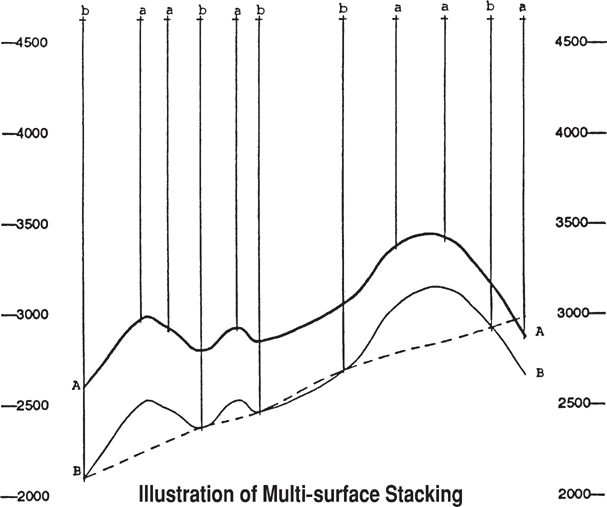
Figure 2-25 Cross section showing stacking process for two surfaces. (AAPG©1991, reprinted by permission of the AAPG whose permission is required for further use.)
Instead, stacking recognizes that there is a true vertical thickness (isochore) value at each of these b points, and the computer program uses them to calculate (interpolate or extrapolate) estimated true vertical thickness values at all of the a points. These calculated thicknesses are subtracted from the elevation of the known Surface A values to get a calculated elevation of Surface B at all of the a points.
A real case will show the benefit of stacking. Figures 2-26 through 2-28 represent a Top-of-Unit structure map, a Unit isochore map, and a Base-of-Unit structure map for the same 13-point sample data set that was used earlier. These maps were made using multisurface stacking. The isochore map was contoured using the five wells that penetrate the Base-of-Unit, interpolating or extrapolating as necessary to cover the entire map area. Then the elevations for the Base-of-Unit at the eight other wells were derived by subtracting the isochore values from the Top-of-Unit elevations. Notice that the Base-of-Unit mimics features of the Top-of-Unit. Highs are shifted in the direction of thinning isochores.
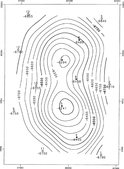
Figure 2-26 Structure contour map on Top-of-Unit. (Published by permission of Scientific Computer Applications, Inc.)
Figure 2-29 shows the same Top-of-Unit and Base-of-Unit and Unit isochore contours all plotted on the same map. It illustrates precisely how a geoscientist would generate a Base-of-Unit map by hand, using the Top-of-Unit map and the Unit isochore map. Note the three-contour crossing points (e.g., wherever the two surfaces, Top-of-Unit and Base-of-Unit, are 100 ft apart, that is a point on the 100-ft isochore).
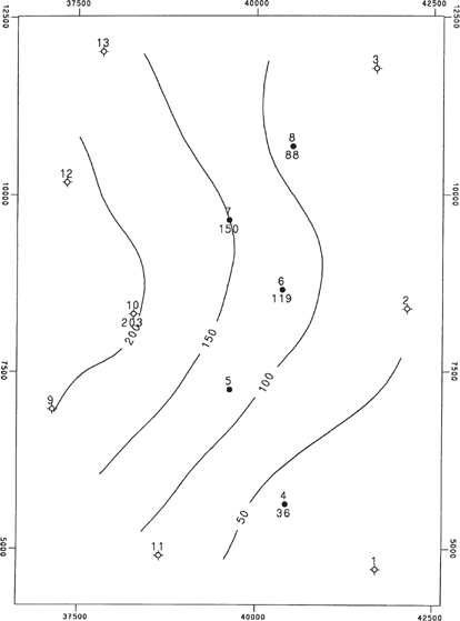
Figure 2-27 Unit isochore map. (Published by permission of Scientific Computer Applications, Inc.)

Figure 2-28 Structure contour map on Base-of-Unit with stacking. (Published by permission of Scientific Computer Applications, Inc.)

Figure 2-29 Top-of-Unit and Base-of-Unit maps and Unit isochore map overlaid. (Published by permission of Scientific Computer Applications, Inc.)
Base-of-Unit has been penetrated by five wells only. If it were processed without the information derived from the 13 wells that penetrate the Top-of-Unit and the knowledge that the surfaces are similar, that is, if it were processed without stacking, we would get a structure contour map as shown in Figure 2-30. If we proceed to make a Unit Isochore by subtracting Figure 2-30 from Figure 2-26, it would be as shown in Figure 2-31. Note that all Unit isochore values are honored, but the interpretation is much different than that shown in Figure 2-28 and is unreasonable if Top-of-Unit and Base-of-Unit are conformable surfaces. The value of stacking is clearly seen when maps with and without stacking are compared.

Figure 2-30 Structure contour map on Base-of-Unit without stacking. (Published by permission of Scientific Computer Applications, Inc.)
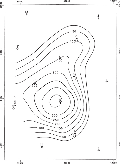
Figure 2-31 Unit isochore map without stacking. (Published by permission of Scientific Computer Applications, Inc.)
Some software programs utilize the concept of multisurface stacking without explicitly creating isochore maps using a concept called conformable gridding. In conformable gridding, data points on the surface being mapped are honored, but the shape of a better-constrained surface is honored in areas away from control points. Conformable gridding mimics multisurface stacking, and isochore maps constructed from conformably gridded surfaces should match traditional isochore maps.
The recent shift to drilling increasing numbers of horizontal or highly deviated wells has allowed us to expand on the concept of multisurface mapping or conformable mapping. With vertical wells, mappers tend to project data points from shallower wells down to deeper horizons. With horizontal wells, we can augment this process by projecting data points from deeper horizons onto shallower horizons. Thompson et al. (2017) recently reported on a workflow, called 2D Conformal Mapping (2DCM), that they use to refine structure maps and help with real-time adjustments to directional wells.
In the workflow outlined by Thompson, tops from multiple surfaces in horizontal wells are compared to structural models constructed using conformable mapping (Fig. 2-32). One horizon is designated a reference horizon, the Horizon A in the case of Figure 2-32. Other horizons are constructed to be conformable with the reference horizon (Thompson et al. 2017). The reference horizon should be carefully selected not only on the availability of well control but also on the presence of a good, mappable seismic event if seismic is available (Vogt, personal communication, 2018). The seismic data provides structural control away from well control, such as on the flanks of a field or in portions of the field not yet developed by drilling. Construction of the reference horizon should be done very carefully, as it influences the mapping of all other horizons. Particular care should be paid to any velocity anomalies that might influence depth conversion of the seismic horizon away from well control, as is discussed in Chapter 5.

Figure 2-32 New horizontal well drilled on existing structural model. The horizon pick at the reference Horizon A matches the existing model, but the two picks of Horizon B and one pick of Horizon C do not match the existing model. (From Thompson et al. 2017. Published by permission of Society of Petroleum Engineers.)
Figure 2-32 shows that the A Horizon pick of the reference horizon ties the existing structural model very well but that picks of Horizons B and C do not tie the existing model. Control points for the reference Horizon A are constructed using the picks on Horizons B and C (Fig. 2-33). These control points are located directly above the horizon picks for Horizons B and C and are shifted from the existing structural model by the same true vertical depth distance that horizon picks B and C are offset from the structural model (Thompson et al. 2017). In Figure 2-33, all of the picks for Horizons B and C are below the existing structural model, but in other cases, the horizon picks could be below or above the existing structural model.
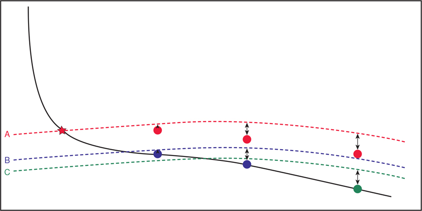
Figure 2-33 Control points for the reference horizon are constructed on the basis of the vertical distance between the deeper horizon picks and the existing structural model. (From Thompson et al. 2017. Published by permission of Society of Petroleum Engineers.)
The reference Horizon A is remapped using all existing data, including the new control points. Horizons B and C are then remapped using conformable mapping with the reference horizon. The actual picks for Horizons B and C from the new horizontal well are excluded from the database when the deeper horizons are remapped (Thompson et al. 2017). The new structural model ties all of the horizon picks in the new horizontal well (Fig. 2-34). With the correct computer software, this remapping can be done in real time as a well is being drilled, allowing real-time adjustment to directional plans for horizontal wells (Thompson et al. 2017).
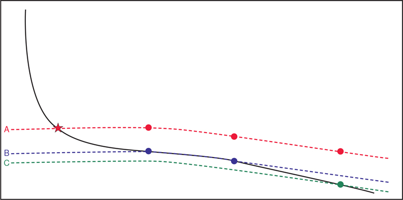
Figure 2-34 The reference Horizon A is remapped using existing data plus the new control points. Deeper Horizons B and C are remapped using the updated reference Horizon A and conformable mapping. (From Thompson et al. 2017. Published by permission of Society of Petroleum Engineers.)
In this example, one horizontal well results in four control points for the reference Horizon A, one actual penetration point, and three control points generated from penetration points of other horizons. Over time, the reference horizon may contain many more control points than actual well penetration points, resulting in a significantly more accurate structure map than using actual well penetrations alone.
Contouring Faulted Surfaces on the Computer
Faults historically have made contouring by hand or computer more complicated because faults destroy the continuity of surfaces being contoured. When contouring faulted surfaces by hand, geologists compensate mentally for fault vertical separation (missing or repeated section) and copy shapes across faults that have structural compatibility. Vertical separation is described in Chapters 7 and 8.
Various schemes have been used in an attempt to teach the computer to be able to contour and display faulted surfaces. One of the simplest is to define the fault by a group of connected vectors that separate data on one side of the fault from data on the other side. No fault surfaces are used in the construction. The mapping of this type of fault information on a structural horizon is sometimes called a trace fault. Data on each side of the fault are contoured separately and extrapolated to the fault. The vertical separation resulting from the fault is implied from data on each side of the trace fault. The fault is displayed as a vertical fault without any fault gap, and shapes are not necessarily copied across the fault. Figure 2-35 shows an example of a trace fault. Note that fault vertical separation is implicit from the data and changes radically. Also note that shape is not copied across the trace fault.
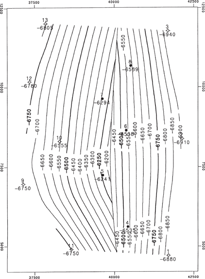
Figure 2-35 Example of trace fault. (Published by permission of Scientific Computer Applications, Inc.)
Another procedure that is used to allow computers to handle faulted surfaces is based on fault polygons. In this procedure the faulted surface is divided into a series of polygons that describe individual fault blocks. Data in each fault block are contoured separately, one surface at a time. Fault vertical separation is implicit and is not treated as an explicit variable. Figure 2-36 is an example of a map contoured using fault polygons.

Figure 2-36 Example of contouring using fault polygons. (Published by permission of Scientific Computer Applications, Inc.)
Another procedure for contouring faulted surfaces on the computer is known as the restored surface method (fault/structure map integration), which is further discussed in Chapters 7 and 8. It is based on contouring both the fault surfaces and their vertical separations. Hence vertical separation (missing or repeated section) is explicit rather than implicit. Figure 2-37 shows a faulted structure map made using the restored surface method and the same data shown in Figures 2-35 and 2-36. Figure 2-38 is contoured on the fault, which has a constant 100 ft of vertical separation.
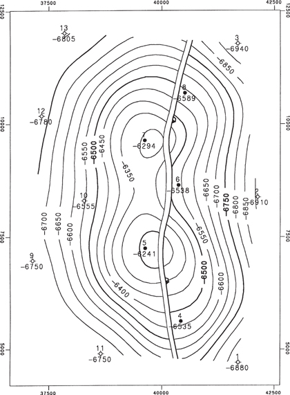
Figure 2-37 Faulted structure using restored surface method. (Published by permission of Scientific Computer Applications, Inc.)
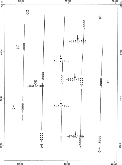
Figure 2-38 Fault surface for 100-ft fault. (Published by permission of Scientific Computer Applications, Inc.)
In this restored surface method, faulted systems are treated as what they are: sets of 3D fault blocks containing mappable strata, which once were continuous surfaces. The boundaries of these fault blocks are the fault surfaces, and they are contourable. The restored surface method is essentially the procedure that is used when contouring faulted surfaces by hand.
In the restored surface method, faulted systems are processed in three steps designed to honor continuity of shape across faults:
Move (i.e., restore palinspastically) the fault blocks, together with the contained geological horizons, to their prefaulted positions.
Having restored the “continuous surface” attribute to the geological horizons, perform all the stacking (discussed earlier) and interpolations needed to obtain a smooth map or cross section.
Rebreak (i.e., reverse the first step) and return the fault blocks and their contents to their faulted positions and display contour maps or cross sections.
Procedure for Contouring Faulted Surfaces.
To accomplish the steps of the restored surface method, certain data are needed. These data consist of:
XYZ data for all horizons (in their faulted position).
Three or more XYZ points for each fault.
Three or more XYZ points for the vertical separation for each fault.
The missing section, or vertical separation, to the computer, is just another mathematical surface, which can vary over the mapped area and can be contoured. Vertical separation is designated as positive for normal faults and negative for reverse faults.
It is valuable to make a mental picture of the faulting process. In order to restore the fault blocks to their prefaulted position successfully, it is helpful to have a reasonable hypothesis about the order in time of the various faulting events, since the most successful restoration to unfaulted positions needs to be done in steps in reverse order to the original faulting. The faulted system normally is analyzed first by making contour maps and/or cross sections of all fault surfaces in order to:
Test the faults for reasonableness. Do observed fault cuts assigned to the same fault result in a fault surface that makes geological sense?
Infer and/or ascertain the hierarchy of the faults with respect to age. Where two faults meet in space and do not cross one another, which one extends beyond that junction? Which one is therefore older? The analysis lends itself to “what if” games regarding the faulting sequence.
To perform its task, the computer can use a set of restore commands, each of which describes a fault block and instructs the program to move it to its prefaulted or restored position. Restore commands take us “backward in time.” The first restore reverses the most recent faulting event; the last restore reverses the oldest faulting event. Geological knowledge must be used to make decisions regarding fault analysis.
We use as an example a sand unit offset by a bifurcating fault system, and we create structure maps of the top and base of the unit. The system consists of two merging faults, Fault A and Fault B, contoured in Figures 2-39 and 2-40. The maps also show the line of bifurcation where Fault B merges with Fault A. Data for these faults were obtained by correlating logs, picking horizon tops, locating faults, and measuring missing sections (vertical separations). Fault A has observed cuts on both sides of the line of bifurcation and Fault B does not, so we conclude that Fault A is the older fault and Fault B is the younger fault. Hence Fault B will be restored first, and then Fault A will be restored. Also, we note that vertical separation of Fault A east of the line of bifurcation is the sum of the vertical separations of Faults A and B west of the line of bifurcation because Fault B no longer exists. Vertical separation balance must be maintained around the line of bifurcation.
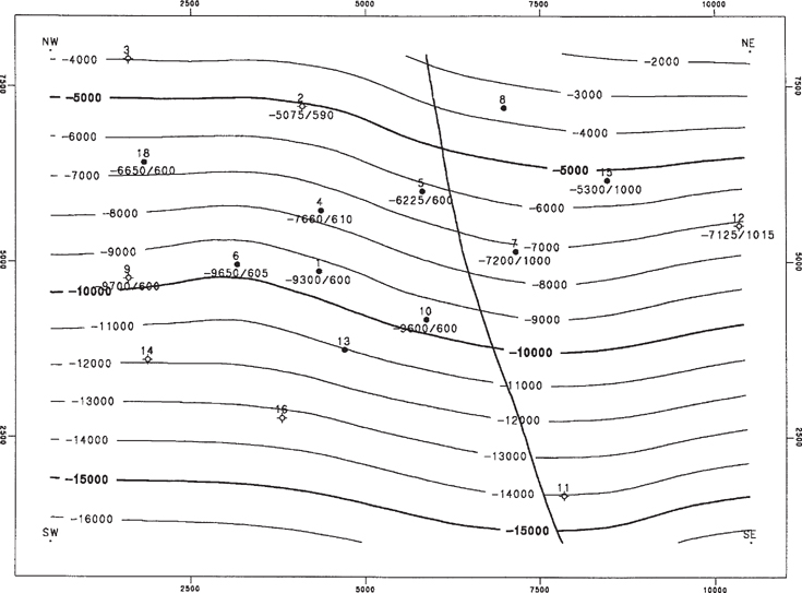
Figure 2-39 Fault surface map of Fault A with vertical separation (missing section) posted. Line of bifurcation with Fault B is shown. (Published by permission of Subsurface Consultants & Associates, LLC.)
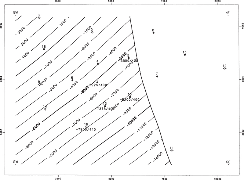
Figure 2-40 Fault surface map of Fault B with vertical separation (missing section) posted. Line of bifurcation with Fault A is shown. (Published by permission of Subsurface Consultants & Associates, LLC.)
Next, we restore the fault blocks to their original unfaulted positions and then contour the paleosurface. Figures 2-41 through 2-43 display conceptually the steps taken by the computer program in restoring the faults. Notice the changes in well depths from figure to figure. Figure 2-41a shows the depths of the Top-of-Unit in the three fault blocks, as separated by the approximate locations of Fault A and Fault B. Figure 2-41b is a north-south cross section before any restoration has occurred. Figure 2-42a is a base map on the Top-of-Unit after Fault B has been restored, and Figure 2-42b is a cross section after Fault B has been restored.
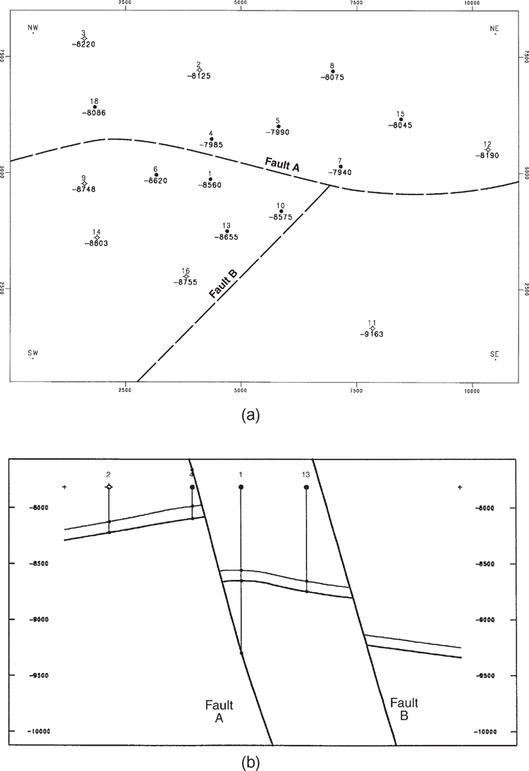
Figure 2-41 (a) Base map with Top-of-Unit elevations and approximate traces of Faults A and B. (b) North-south cross section before restoration of faults. (Published by permission of Subsurface Consultants & Associates, LLC.)
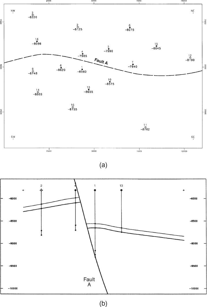
Figure 2-42 (a) Base map of Top-of-Unit after Fault B has been restored. (b) North-south cross section after Fault B has been restored. (Published by permission of Subsurface Consultants & Associates, LLC.)
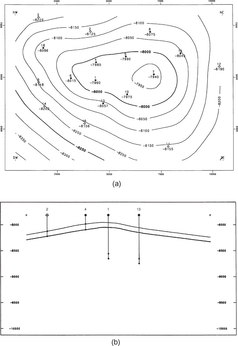
Figure 2-43 (a) Structure map of Top-of-Unit contoured after Fault A has been restored. This is the paleosurface prior to faulting. (b) North-south cross section after Fault A has been restored. (Published by permission of Subsurface Consultants & Associates, LLC.)
Next, we restore the block moved during fault event A (the block downthrown to Fault A), which incidentally contains restored Fault B. That restoration produces an unfaulted surface, which is the paleosurface prior to all faulting. We then contour that surface. Figure 2-43a is a structure map of the Top-of-Unit that was contoured after Fault A was restored. Figure 2-43b shows the paleosurfaces in cross section.
Now that the faulted system has been restored to its prefaulting configuration, the structural surfaces are continuous and can be stacked, as described earlier in this chapter.
The final step in processing faulted surfaces is to rebreak and move geological surfaces to their true (postfaulted) positions. This step is the mathematical inverse of restoration. In the restored surface method, the computer program generates hanging wall and footwall fault traces as the intersection between structural horizons and faults. Rigorous vertical separation balance should be maintained at all fault intersections. In our example, the structure contour maps for Top-of-Unit and Base-of-Unit are completed and shown in Figures 2-44a and b.

Figure 2-44 Completed structure maps of (a) Top-of-Unit, and (b) Base-of-Unit, after surfaces have been moved to their true postfaulted positions. (Published by permission of Subsurface Consultants & Associates, LLC.)
Limitations.
Limitations of the restored surfaces method as implemented by the computer have their origin in mathematical simplifications, the most important of which is the use of purely vertical movement in the fault restoration process. This implies that the method becomes less applicable when fault movement is essentially horizontal, for example, strike-slip or very low-angle thrust faults.