Chapter 4. Log Correlation Techniques*
* For all figures in this chapter (in the printed book only), see the preface for information about registering your copy on the InformIT site for access to the electronic versions in color.
Introduction
Correlation can be defined as the determination of structural or stratigraphic units that are equivalent in time, age, or stratigraphic position. For the purpose of preparing subsurface interpretations, including maps and cross sections, the two general sources of correlation data are electric wireline or LWD (logging-while-drilling) logs and seismic sections. In this chapter, we discuss basic procedures for correlating well logs, introduce plans for performing various phases of well log correlation, and present fundamental concepts and techniques for correlating well logs from vertical as well as directionally drilled wells.
Fundamentally, electric well log curves are used to delineate the boundaries of subsurface units for the preparation of a variety of subsurface maps and cross sections (Doveton 1986). These maps and cross sections are used to develop an interpretation of the subsurface for the purpose of exploring for and exploiting natural resources, including hydrocarbons.
After the preparation of an accurate well and seismic basemap, electric log and seismic correlation work is the next step in the process of conducting a detailed geological/geophysical study. No geological interpretation can be prepared without detailed correlations. Accurate correlations are paramount for reliable geological interpretations.
General Log Measurement Terminology
An understanding of several log depth measurements is important for converting log depths to depths used in mapping. The following is a list of measurements, their abbreviations, and definitions of depth terminology. These terms are illustrated in Figure 4-1.

Figure 4-1 Diagram showing general log measurement terminology.
KB |
Vertical distance from kelly bushing to sea level. The kelly bushing is the most common reference for measuring logs. The rig floor (RF) or derrick floor (DF) or rotary table (RT) are other common reference points. |
MD |
Measured depth. Measured distance along the path of a wellbore from the kelly bushing to TD (total depth of the well) or any correlation point in between. May also be called along hole depth (AHD) (Brooks et al. 2005) or true along hole depth (TAH) (Forsyth et al. 2013). |
TVD |
True vertical depth. Vertical distance from the kelly bushing to any point in the subsurface. |
SSTVD |
Subsea true vertical depth. Vertical distance from sea level to any point in the subsurface. SSTVD may either be positive (above sea level) or negative (below sea level). |
Vertical Wellbore |
A well drilled 90 deg to a horizontal reference, usually sea level (also called a straight hole). |
The SSTVD measurement is the only depth measurement from a common reference datum, sea level. Therefore, SSTVD is the depth most often used for mapping. Logging depths measured from a vertical or directionally drilled well for mapping are usually corrected to SSTVD. For vertical wells, the SSTVD = KB − TVD. The measurements for directionally drilled wells are discussed in Chapter 3.
Electric Log Correlation Procedures and Guidelines
What is well log correlation? Electric log correlation is pattern recognition. It is often debated whether this pattern recognition is more of an art or a science, but we believe both play a part in correlation work. Professionals involved with log correlation must be well versed in sound geological principles, including depositional processes and environments, and have an understanding of the tectonic setting under study. They should also be familiar with the principles of logging tools and measurements, general reservoir engineering fundamentals, and basic qualitative and quantitative log analyses.
The best way to develop log correlation ability is by actually performing correlation work. A geologist should become more proficient with increased experience in correlation. Proficiency in correlating well logs in one tectonic setting or depositional environment does not always ensure similar competence in other settings. In other words, someone who is an expert at correlating well logs in the South American Andes Mountains Overthrust may not be equally competent when working in, for example, Offshore West Africa. Just as it took time to become proficient at correlating logs in the South American Andes, so too will it take time and familiarity in the new area to become proficient.
When geologists correlate one log to another, they are attempting to match the pattern of curves on one log to the pattern of curves found on the second log. A variety of curves may be represented on a log. For correlation work, it is best to correlate well logs that have the same type of curves; however, this is not always possible. A geologist may be required to correlate logs that have different curves. And at times, even if the logs have the same curves, the character or magnitude of the fluctuations of the curves may be different from one log to the next. Therefore, the correlation work must be independent of the magnitude of the fluctuations and the variety of curves on the individual well logs. Figure 4-2 shows sections from two electric logs. The patterns of curves on Well No. A-1 are very similar to the patterns on Well No. A-2. We can say that these two logs have a high degree of correlation.
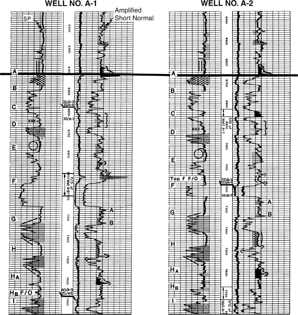
Figure 4-2 Portion of two electric logs illustrating methods of annotating recognizable correlation patterns on well logs.
The data presented on a well log are representative of the subsurface formations found in the wellbore. A correlated log provides information about the subsurface, such as stratigraphic markers, tops and bases of stratigraphic units, depth and amount of missing or repeated section resulting from faults, lithology, depth to and thickness of hydrocarbon-bearing zones, porosity and permeability of productive zones, and depth to unconformities. The information obtained from correlated logs is the raw data used to prepare subsurface interpretations and maps. The maps may include fault, structure, stratigraphic, salt, unconformity, and a variety of isochore maps. These data can also be used to prepare a variety of cross sections. Accurate correlation is the foundation of reliable subsurface interpretations. Subsurface geological maps based on log correlation are only as reliable as the correlations used in their construction. Eventually, a geologist’s correlations, right or wrong, are incorporated into the construction of subsurface geological maps. An incorrect correlation can be costly in terms of a dry hole or an unsuccessful workover or recompletion; therefore, it is essential that extreme care be taken in correlating well logs.
In this section, we introduce you to a general correlation procedure and discuss some guidelines for electric log correlation. The process of correlating logs varies from one individual to the next. As geologists gain experience, they modify and eventually establish a correlation procedure that works best for them. If you have no experience in log correlation or want to improve your skills, you can begin by using the procedures and guidelines discussed in this section.
Electric logs can be correlated by hand or with the assistance of a computer. When correlated by hand, the electric logs are arranged on a worktable in one of two ways (Fig. 4-3). The arrangement shown in Figure 4-3a is preferred over that shown in Figure 4-3b by most geologists because more log section can be viewed at one time and the logs are easier to slide during correlation. The manipulation of logs on a computer screen is described in the section Computer-Based Log Correlation.
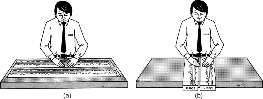
Figure 4-3 (a) Preferred method of arranging logs for correlation. (b) Alternate method of arranging logs for correlation.
As a starting point, align the depth scale of the logs and look for correlation, as shown in Figure 4-2. If no correlation is evident, begin to slide one of the logs until a good correlation point is found, and mark it. Continue this process over the entire length of each log until all recognized correlations have been identified. This process may seem relatively easy, but it can be complicated by such factors as stratigraphic thinning, bed dip, faulting, unconformities, lateral facies changes, poor log quality, and directionally drilled wells. If seismic data is available near the wells being correlated, it should be consulted prior to beginning correlating. Many of the complicating factors listed above may be apparent on the seismic, which will make correlating easier and more efficient.
There are some basic, universally valid guidelines, which are useful in the log correlation process. If followed, these guidelines should improve your correlation efficiency and minimize correlation problems.
For initial quick-look correlation, review major sand or carbonate bodies using the spontaneous potential (SP) curve or gamma ray (GR) curve.
For detailed correlation work, first correlate shale sections.
Initially, use the amplified shallow resistivity curve (focused, short normal, or shallowest reading array induction), which usually provides the most reliable shale correlations.
Use colored pencils to identify specific correlation points.
Always begin correlation at the top of the log, not the middle.
Correlate the entire log.
Do not force a correlation.
In highly faulted areas, first correlate down the log and then correlate up the log.
After an initial quick look using the SP curve or GR curve to identify the major sand or carbonate bodies, concentrate your correlation work on shale sections. There are three good reasons for this. First, the clay and silt particles that make up shales are deposited in low-energy regimes. These low-energy environments responsible for shale deposition commonly cover large geographic areas. Therefore, the log curves (sometimes referred to as log signatures) in shales are often highly correlatable from well to well and can be recognized over long distances. Second, prominent sand bodies are often not good correlation markers because they commonly exhibit significant variation in thickness and character from well to well and are often laterally discontinuous. Finally, the resistivity curves for the same sand on two well logs being correlated may be different. Variations in fluid content in a sand bed may cause pronounced resistivity differences (e.g., water versus gas).
Individual shale beds exhibit distinctive resistivity characteristics over large areas. Therefore, when all log curves are considered, the amplified shallow-investigation resistivity curve provides the most reliable shale correlations. Although all log curves should be used for correlation work, the amplified resistivity curve is five times more sensitive than the unamplified curve and exhibits patterns that are easier to recognize and correlate from well to well. The amplified curve should be the initial curve used for correlation (Fig. 4-2).
The liberal use of colored pencils is an excellent way to identify and mark correlation patterns on well logs. The correlation patterns might be peaks, valleys, or groups of wiggles that are recognizable in many or all of the well logs being correlated (Fig. 4-2). The colored pencils should be erasable in the event that correlations are changed. Do not mark on original logs. A blueline or blackline copy of the original logs should be used for marking during correlation.
In general, structures become less complicated toward the surface because of several factors. Many faults tend to die upward toward the surface and are either small or nonexistent in the upper part of the logs. This makes for easier correlations. Also, in many geological provinces, especially in soft rock basins, the structural dip, both local and regional, decreases upward. Therefore, beginning correlation at the top of a log is usually easier.
Correlations are not always straightforward and everyone runs into correlation problems from time to time. Often there is a tendency to force a correlation rather than bypass the problem area until further work is done. This is not good practice. Correlation problems are commonly due to the presence of faults, high bed dips, unconformities, and facies changes. It is best to pass the problem area and continue the correlation work on the remaining section of the log. Later, when the remainder of the problem log and other logs have been correlated, the questionable correlations can be reviewed again with this new information.
In highly faulted areas it is advantageous to approach a recognized fault from two directions. First, correlate down the log to the fault and then correlate up the log to the fault. By taking this approach, determination of the amount of missing or repeated section and depth of the fault in the correlated well will be more accurate (Figs. 4-2 and 4-10). This method is discussed in detail later in this chapter.
Correlation Type Log
A correlation type log is defined as a log that exhibits a complete stratigraphic section in a field or regional area of study. The type log should reflect the deepest and thickest stratigraphic section penetrated. Because of faults, unconformities, and variations in stratigraphy affecting the sedimentary section, a correlation type log is often composed of sections from several individual logs and is referred to as a composite type log.
Do not confuse a correlation type log with other kinds of type logs, such as stratigraphic type logs, composite sand type logs, or show logs. A stratigraphic type log is usually prepared to depict the depositional environments that existed in a particular field or area of study (Fig. 4-4). Although it may include portions of several logs to depict the entire stratigraphic section, it is usually not prepared in the strict sense of a correlation type log. Therefore, it may contain faults or unconformities and include sections of wells near the crest of the structure, which do not represent the thickest sedimentary section.
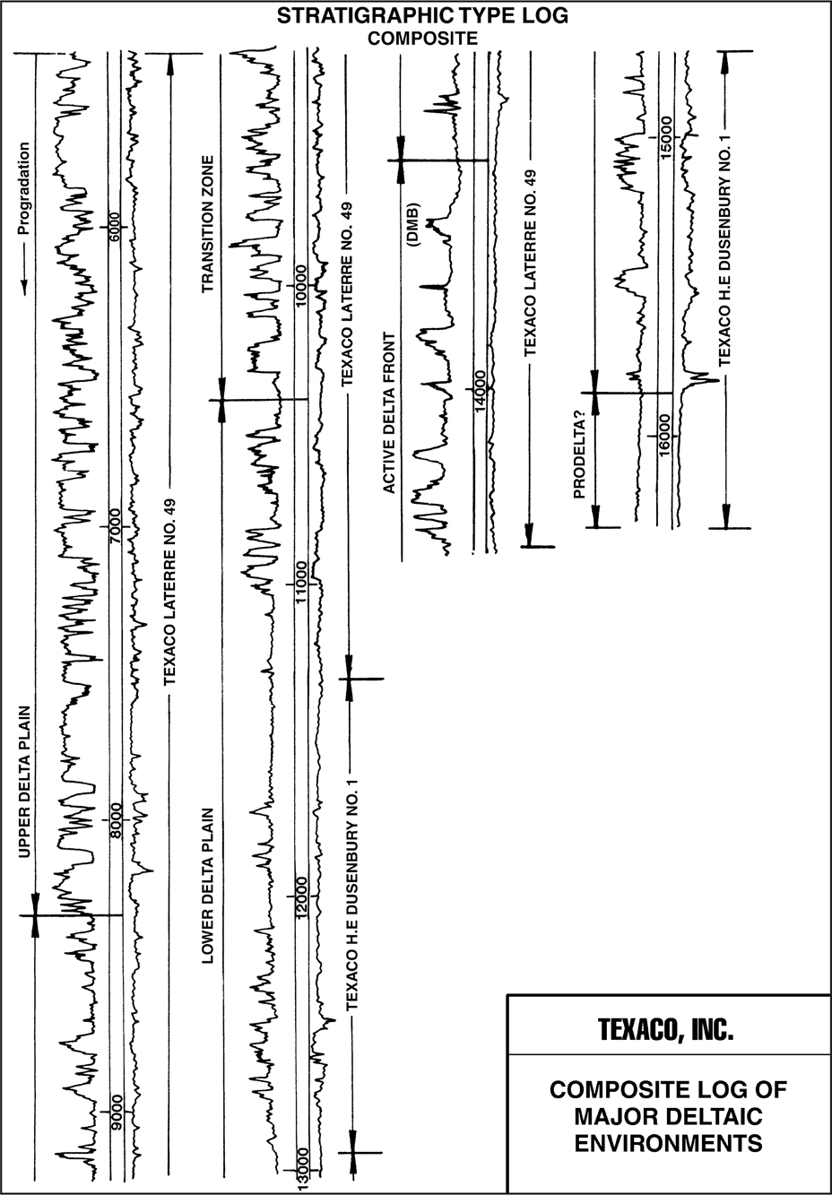
Figure 4-4 Composite stratigraphic type log. (Published by permission of Texaco USA.)
Composite pay logs or show logs are prepared to illustrate the potential productivity within a field or area of study that have shows, contain hydrocarbons, or have the potential to be hydrocarbon bearing (Fig. 4-5). These logs are not prepared for use as a correlation aid and therefore are not prepared in the rigid manner of a correlation type log.
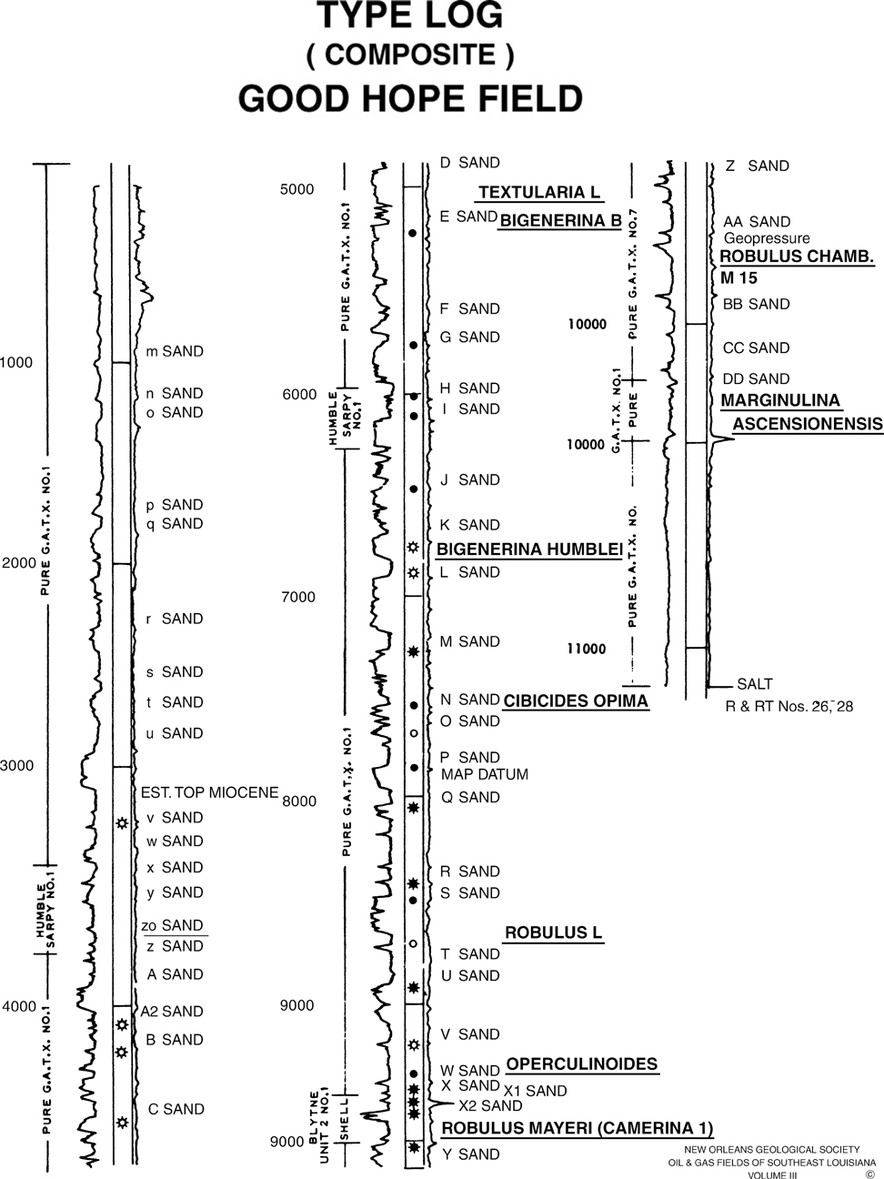
Figure 4-5 Composite show log from Good Hope Field, St. Charles Parish, Louisiana. (Published by permission of the New Orleans Geological Society.)
When beginning geological work in a new area of study in which a type log has already been prepared, it is important to carefully review the log to see that it meets with the requirements of a correlation type log. If the type log has an incomplete stratigraphic section, its use will result in correlation errors. The type log must have the complete stratigraphic section if it is to be a useful tool for correlation.
Figure 4-6 shows a cross section through a complex diapiric salt structure. We use this figure to illustrate the procedure for preparing a correlation type log. This structure exhibits a number of complexities, including a salt overhang, several faults, an unconformity, diapiric shale, stratigraphic thinning, and stratigraphic pinchouts in the up-structure position near the salt. We consider each of the four wells that have penetrated the structure and evaluate the applicability of each as a type log.

Figure 4-6 A cross section through a complex diapiric salt structure, penetrated by four vertical wells.
Well No. 1 is not a good candidate as a type log for several reasons: it reaches a depth of only −8700 ft, crosses a crestal fault, encounters salt at a shallow depth, and does not penetrate a complete section. Well No. 2 is drilled off the flank of the structure and penetrates a thick, nearly complete stratigraphic section. However, it crosses an unconformity at about −11,300 ft. Well No. 3 is also drilled in a down-dip position and penetrates the entire stratigraphic section before encountering diapiric shale near the total depth (TD) of the well. However, it crosses a fault at about −10,500 ft in the 9100-ft Sand. Well No. 4 drilled in a crestal position is not suitable as a type log because it penetrates the salt overhang, encounters a thinner stratigraphic section than that penetrated by Wells No. 2 and 3, crosses a fault and an unconformity, and does not penetrate a complete stratigraphic section.
For this particular example, the correlation type log must be a composite log including sections from Wells No. 2 and 3. The best type log consists of Well No. 2 from the surface down to a correlation marker just below the 11,000-ft Sand and Well No. 3 from the same marker to TD in diapiric shale. This composite type log meets all the requirements in the definition shown earlier and is an excellent standard for all other well log correlation work on this structure.
Normally, faults are not included on a correlation type log. However, if a major decollement, such as a thrust or listric growth fault, serves as the deepest limit of prospective section, it is advisable to place the fault on the type log.
Electric Log Correlation—Vertical Wells
We begin the discussion of actual correlation work by reviewing electric log correlation in vertical wells. In general, electric log correlation is easier and more straightforward in vertical wells than in wells that are directionally drilled. Later in this chapter, after we discuss the fundamental concepts and techniques of correlation in vertical wells, we review the same concepts and techniques as they apply to directionally drilled (deviated) wells.
Log Correlation Plan
When given the task of correlating logs in a specific field or area of interest, you might ask yourself one of several questions: “Where do I start?” or “Which log do I correlate first, second, third, etc.?” Before starting the log correlation in an area, a general log correlation plan needs to be developed. In this section, we illustrate a log correlation plan that provides an answer to the questions asked and establishes a preferred order in which to correlate electric logs from vertically drilled wells. This correlation plan can be adapted to most geological settings. For the purpose of illustration, we use a structure map of the 8000-ft Horizon on a normally faulted anticlinal structure in an extensional geological setting (Fig. 4-7). Considering the faults on the anticline in the up-dip position, the structure becomes more complex in the up-dip direction.
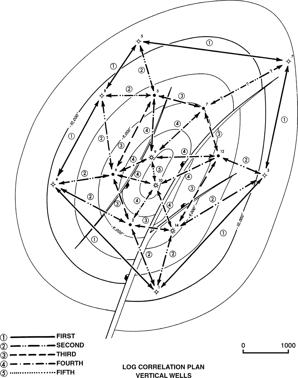
Figure 4-7 An example of a log correlation plan for vertical wells. Notice that there is a hierarchy in the correlation sequence and that all the wells are correlated in closed loops.
The following log correlation plan is intended to make correlation work more systematic and easier to conduct and to result in fewer difficulties in correlation.
Step 1. First, prepare a correlation type log. Remember that a correlation type log must show a complete unfaulted interval of sediments representative of the thickest and deepest sedimentary section in the field. For the structure in Figure 4-7, the wells furthest off structure, such as Well No. 5 or 7 or a composite of the two, are good candidates for a type log if these wells are drilled deeply enough. These wells, positioned off the crest of the structure, should show the thickest and most complete sedimentary section.
Step 2. A good correlation plan involves the correlation of each well with a minimum of two other wells. To ensure good correlation efficiency over the entire area, the plan should be established to correlate by means of closed loops. The correlation plan in Figure 4-7 illustrates a sequence of closed loops. The recommended order of correlation is represented by “billiard ball” type numbers for correlation sequence. Using this procedure, the log correlation work within a loop begins and ends with the same log, eliminating correlation mis-ties and reducing the chance of other correlation errors.
Step 3. First correlate wells expected to exhibit the most complete and thickest stratigraphic section. On a structure such as the one shown in Figure 4-7, the structurally lowest wells usually have the thickest section. These include wells represented by the billiard ball type correlation sequence number 1.
Step 4. Continue log correlation, progressing from wells in a down-structure position to wells in an up-structure position (see the billiard ball type correlation sequence numbers 2, 3, 4, and 5). These numbers indicate the recommended correlation sequence for the example.
Step 5. Generally, correlate wells located nearest each other. In most cases, closely spaced wells should have a similar stratigraphic section and so correlation is usually easier.
Step 6. In many geological areas, rapid changes in stratigraphy (particularly changes in thickness) occur over short distances. Where possible, correlate wells anticipated to have a similar stratigraphic interval thickness. In extensional or diapiric tectonic areas, wells at or near the same structural position often exhibit similar stratigraphy. For areas involving plunging folds, similar stratigraphy may be exhibited along the plunge of the fold.
Also, if wells that exist at or near the same structural bend are connected together, as in the first order correlation as shown in Figure 4-7, the dip rate of the structure should be similar in these various wells, thus eliminating correlation problems related to changing structural dip.
In geological settings containing syndepositional faults (commonly referred to as growth faults), some special considerations must be given in preparing a log correlation plan. For our purposes, we define a growth normal fault as a syndepositional fault resulting in an expanded stratigraphic section in the hanging wall fault block, with missing section on the growth fault changing with depth.
If a growth fault is present in the area of study, restrict the correlation to wells within one fault block of the growth fault. Keeping in mind that the hanging wall block of a major growth fault has an expanded stratigraphic section, which can increase the difficulty in correlation, start the correlation in the footwall block using the plan just outlined. Once the correlations are completed in the footwall fault block of the major growth fault, carry the correlations, if possible, into the hanging wall fault block. Initially, check the correlation in wells located in down-structure positions.
If a significant amount of growth has occurred on the fault, the thickness of the sediments can be so great in the hanging wall block that correlation of the section from hanging wall to footwall blocks may be difficult, if not impossible. In such a case, the best correlations can be achieved by preparing a separate type log for the hanging wall block and correlating this fault block independently from the footwall block.
We note here that other terminology is at times used in place of hanging wall and footwall. For a normal fault, the hanging wall is also referred to as the downthrown fault block. As well, the footwall block can be referred to as the upthrown fault block.
Basic Concepts in Electric Log Correlation
Now that we have established a plan of correlation, we examine some basic concepts of electric log correlation. Figure 4-8 shows the SP and amplified short normal resistivity curve from the electric logs of two vertical wells. Initial quick-look correlations can be made by reviewing major sands. Sands are the dominant and most obvious features seen on the SP curve or GR curve and serve as good quick-look correlations. Because sand bodies commonly exhibit significant variation in thickness and character from well to well and are often laterally discontinuous, they are not recommended for detailed electric log correlations.
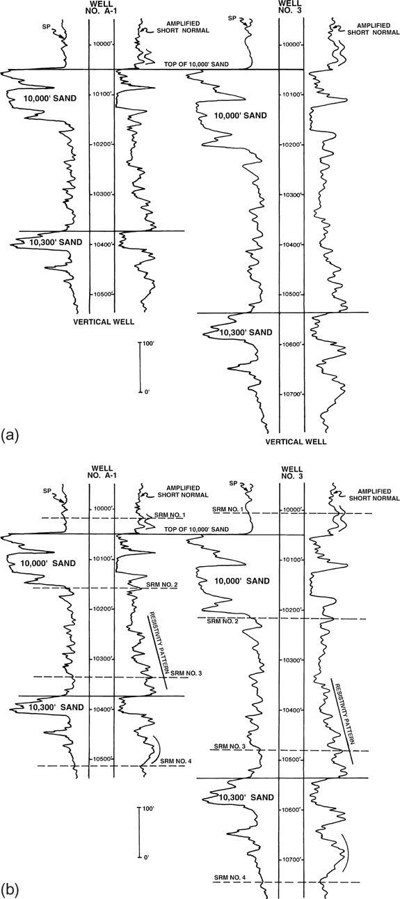
Figure 4-8 (a) Correlation of two vertical wells using the major sands as the primary vehicle for correlation. (b) Detailed correlation of the two vertical wells shown in Figure 4-8a using all the reliable shale and sand correlation markers. (SRM = shale resistivity marker.)
We suggest that all detailed electric log correlation be undertaken by concentrating on shale sections. We apply this approach to electric log correlation in Figure 4-8, which shows a log segment from two vertical wells (No. A-1 and No. 3). The SP and amplified short normal resistivity curves are shown for each log. There are two major sands seen in each well, labeled 10,000-ft Sand and 10,300-ft Sand.
First we review these two logs using the tops of the major sands as the primary vehicle for correlation (Fig. 4-8a). Imagine that we prefer to correlate major sand bodies and we are correlating Wells No. A-1 and 3 in Figure 4-8a. By correlating the sands, we see that the interval from the top of the 10,000-ft Sand to the top of the 10,300-ft Sand is about 325 ft thick in Well No. A-1 and 480 ft in Well No. 3. The interval in Well No. A-1 is short between the two sand tops by 155 ft. This short interval, based on the sand correlations, suggests the possibility of a 155-ft normal fault in Well No. A-1.
Now we correlate these same two logs, shown in Figure 4-8b, using the guidelines outlined earlier. The guidelines recommend that detailed correlations be conducted in the shale sections using all the electric log curves with an initial emphasis on the amplified resistivity curve. This curve provides the most reliable shale correlations.
Through detailed correlations of the shale sections and the sands, a number of correlation markers are identified on the two logs. These include a series of shale resistivity markers (SRMs) labeled SRM No. 1 through SRM No. 4, with certain diagnostic resistivity correlation patterns highlighted on the resistivity side of the logs, in addition to the two major sands. All these correlation markers indicate that both log segments have a high degree of correlation and that no fault is present in Well No. A-1.
It appears that the stratigraphic section in Well No. A-1 is uniformly thin relative to Well No. 3. The thickness ratio for the intervals between each of the four shale markers shows a consistency in the stratigraphic thinning in Well No. A-1 when compared to Well No. 3. This uniform thinning supports the idea that although Well No. A-1 is short to No. 3 as a result of stratigraphic thinning, the two logs exhibit correlation.
Faults Versus Variations in Stratigraphy
We begin the log correlation section to determine faults in an extensional setting where faults typically create a missing section on well logs. The differentiation between recognizing faults versus variations in stratigraphic thickness in well log correlation is very important. We stated earlier that reliable interpretations presented on maps and cross sections are bedrocked in accurate correlations. If a stratigraphically thin section is correlated incorrectly as a fault, this erroneous fault data will be incorporated into the construction of a fault surface map and later integrated into the structural interpretation. The purpose of this section is to outline procedures that are effective during correlation to help differentiate between faults and variations in stratigraphic thickness.
Fault Determinations: Depth and Missing Section.
Now that we have a basic understanding of how shale markers are used to aid in log correlation, look at the log segment from two other electric logs run in vertical wells (Wells No. 1 and 3 in Fig. 4-9). Some geologists prefer to correlate major sands. If we do that and use the 8600-ft and 9000-ft Sands as the principal correlations, we see that the section in Well No. 3 between the two major sands is 80 ft short and a fault appears possible in the well. With the limited correlation data, the missing section and depth of the fault is uncertain. Also, the correlation of the top of the 9000-ft Sand in Well No. 3 is questionable. Is there a fault in Well No. 3, and is the fault (1) within the shale interval between the base of the 8600-ft Sand and the top of the 9000-ft Sand or (2) at the top of the 9000-ft Sand, or (3) is part of the 9000-ft Sand faulted out? If the fault is above or at the top of the 9000-ft Sand, then the interval from the 8600-ft Sand to the top of the 9000-ft Sand is 80 ft short. If part of the top of the 9000-ft Sand is faulted out, then the interval is short by some amount greater than 80 ft. With the major sand correlation methodology, the nature of the short section in Well No. 3 is not apparent, and so we have a correlation problem.

Figure 4-9 Correlation of the major sands in two vertical wells may provide insufficient correlation data to accurately determine the depth and size of a suspected fault.
Now we will follow the recommended correlation procedures illustrated in Figure 4-10. These procedures provide a number of correlation markers, including SRMs 1 through 7 and specific resistivity characteristics highlighted on the resistivity curve of each log. These detailed correlation markers show that the interval between each correlation marker is comparable in both wells except for the short section identified between SRM 5 and SRM 7. Notice that SRM 6 is missing in Well No. 3, as is the lower segment of the resistivity character highlighted through SRM 6 in Well No. 1. Finally, these detailed shale correlations and the correlation data contained within the 9000-ft Sand indicate that the upper portion of the 9000-ft Sand is also missing in Well No. 3. We have isolated the short section in Well No. 3 to a specific interval 135 ft thick. The isolation of this short section to one particular location indicates that the short section is the result of a fault rather than a variation in stratigraphy. The location of the short section provides the depth of the fault in this well. By measuring the amount of section in Well No. 1 that is missing in Well No. 3, we determine the missing section due to the fault (135 ft) by correlation with Well No. 1. The missing section is highlighted in Figure 4-10. In order to ensure confidence in the fault, Well No. 3 should be correlated with at least one more nearby well.
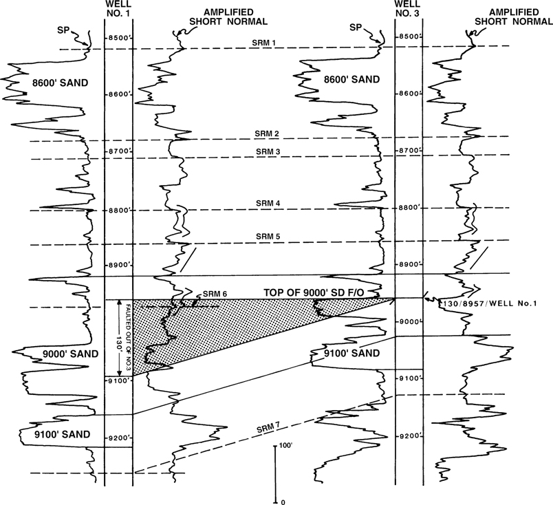
Figure 4-10 Detailed correlation of the two vertical wells shown in Figure 4-9 using all recognizable correlation markers to determine the depth and missing section for a fault in Well No. 3. Notice that the top of the 9000-ft Sand and SRM 6 are faulted out of Well No. 3.
For each fault recognized in a well, there are three important pieces of data that must be obtained for documentation and later use in mapping: (1) the amount of missing section, (2) the depth of the fault in the log, and (3) the well or wells correlated to identify the fault. The fault data (135 ft/8957 ft/Well No. 1) and information regarding the faulted out (F/O) top of the 9000-ft Sand are annotated next to the fault symbol on the log. Refer to Figure 4-10 again for an example of how these data are annotated on a log. For convenience, in most of our examples we use measured well depths for faults and other points. For your mapping purposes, we recommend that you annotate subsea depths.
Most computer-based log interpretation systems automatically record the depth of the fault and provide a specific place in the computer database to record the amount of missing section associated with the fault. Few computer-based log interpretations systems provide a specific place in the computer database to record the well or wells correlated to identify the fault. The geoscientist correlating the logs will usually have to enter this information as an unstructured annotation in the database. We strongly recommend that interpreters take the additional time to add this information, as it makes checking the fault interpretation much easier in the future.
The accuracy of identifying the depth of a fault in a well and determining the amount of missing section is directly related to (1) the detail to which the logs are correlated, (2) the number of logs used for correlation, and (3) variations in stratigraphic thickness seen in the wells. Obviously, the smaller the interval between established correlation markers, the more precise the correlation in pinpointing the depth of the fault in the well and the amount of missing section. Missing section can be incorrectly estimated if the reference well is of different thickness than the faulted well. A thickness ratio can be used to appropriately adjust the amount of missing section that is measured in the reference well log (see following section, Stratigraphic Variations).
The correlation detail and accuracy required are often dictated by the type of geological study being conducted. For example, if you are involved in a regional geological study, pinpointing the depth of a fault within several hundred feet on a well log may be sufficient. Also, you may be interested only in the larger faults (i.e., faults greater than 100 ft). If the study is to be detailed for field development or enhanced recovery, however, it may be necessary to locate the depth of all recognizable faults to within ± 20 ft. The same variation in accuracy applies to missing section as well.
Stratigraphic Variations.
Figure 4-11 shows a log segment from Wells No. A-1 and 3. In this section, we use the correlation procedures to establish specific correlation markers to recognize stratigraphic variations so that such thickness changes are not mistaken for faults.
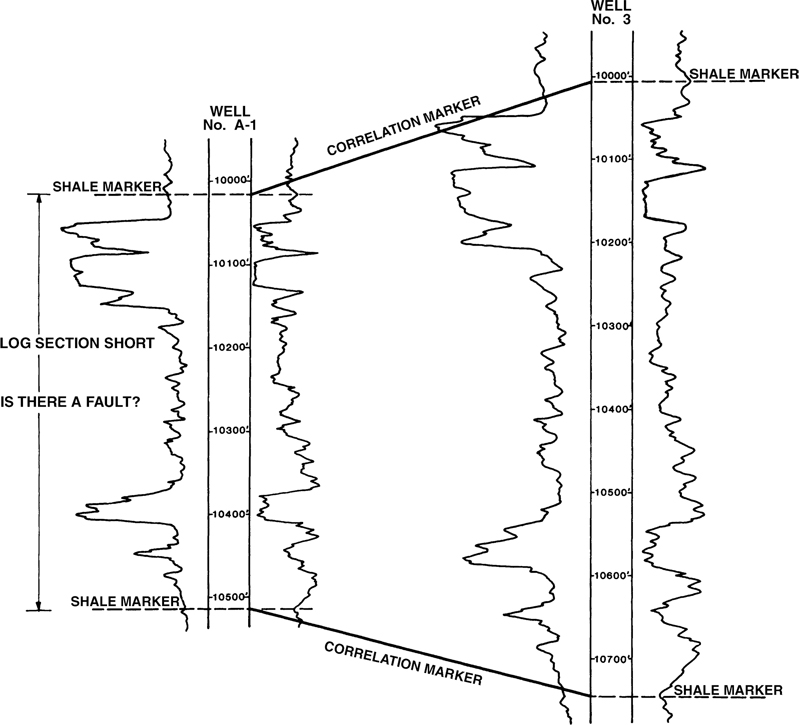
Figure 4-11 Correlation of Wells No. A-1 and 3 using limited correlation markers. Is there a fault in Well No. A-1?
In Figure 4-11, two correlation markers are identified in each well. Based on these markers, Well No. A-1 is 155 ft short to Well No. 3. Is the short section in Well No. A-1 the result of a fault or variations in stratigraphy? With the limited correlation data shown in the figure, it is impossible to determine why the section in Well No. A-1 is short. We could use the major sands in each well to aid the correlation work, but this added information provides little help in determining the nature of the short section.
So far, we have shown that it is important to identify as many correlation markers as possible, especially in questionable log intervals. Closely spaced correlations generally improve the accuracy of the correlation, help differentiate faults from stratigraphic variations, and improve the estimate for the amount of missing section and depth of identified faults. Therefore, in order to accurately correlate Wells No. A-1 and 3, additional correlation markers are required.
Figure 4-12 shows the same two logs with additional correlation markers identified. The correlation process is improved with these additional markers. Notice that the shortening in Well No. A-1 is not isolated to one specific interval but is present in all the intervals in the well between SRM 1 and SRM 4. This evidence strongly suggests that the thickness variations in Well No. A-1 are stratigraphic and not the result of faulting. If necessary, interval thickness ratios can be calculated between correlation markers to provide further evidence to support the conclusion.
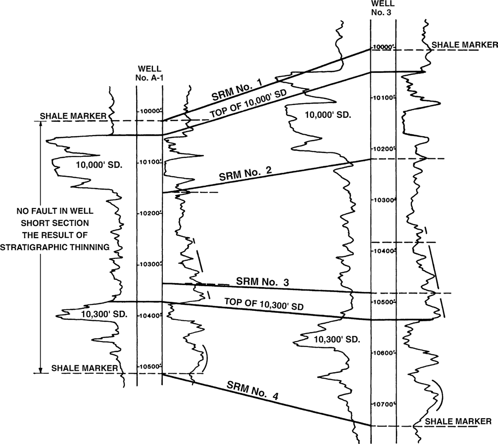
Figure 4-12 Correlation of Wells No. A-1 and 3 using all recognizable correlation markers indicates that there is no fault in Well No. A-1. The short log section is the result of variations in stratigraphy.

where

Pitfalls in Vertical Well Log Correlation
As a final topic on well log correlation in vertical wells, we look at some pitfalls caused by changes in formation dip. Figure 4-13a shows an electric log section from four vertical wells. Using the detailed correlation procedures, we determine that the stratigraphic section shown in each well is the same section. From right to left in the figure, the well logs show an increasing thickness in the section from 100 ft in Well No. 4 to 200 ft in Well No. 1. What is the cause of thickness change in this section: variations in stratigraphic thickness, faulting, or something else?
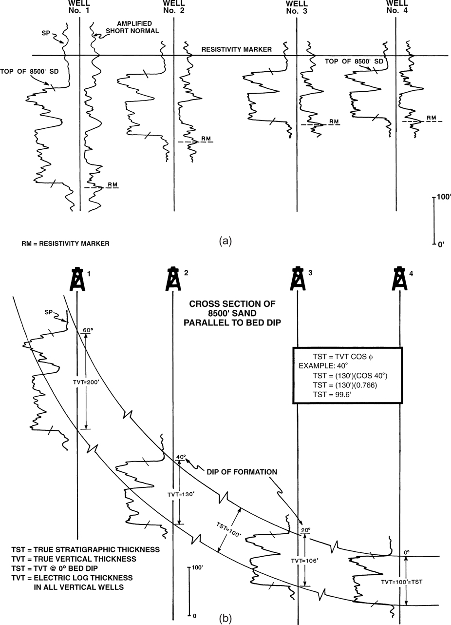
Figure 4-13 (a) Electric log stratigraphic section laid out perpendicular to the strike of the 8500-ft Sand (parallel to dip). (b) Electric log section showing the relationship of TST to TVT with changing bed dip. The TVT is that thickness seen in a vertical or straight hole.
General structure mapping and dipmeter data show that the bed dip is different in the vicinity of each well: 0 deg in Well No. 4, 20 deg in Well No. 3, 40 deg in Well No. 2, and 60 deg in Well No. 1. All four wells lie in a line perpendicular to bed strike (parallel to bed dip). Analysis of the dip data and logs suggests an increase in thickness of the stratigraphic section in the up-structure direction. Normally, however, we expect to see a constant or reduced thickness of a stratigraphic section in the up-structure direction. So, are these thickness changes seen on each log due to faulting, stratigraphic variations, or a geometric problem resulting from changing bed dip?
In Figure 4-13b, the logs are hung in their true structural position with the dip of the formation at each well location shown. The formation dips and the relationships between true bed or stratigraphic thickness and log or vertical thickness are shown on the figure. Notice that even though the log thickness in Well No. 1 is twice that seen in Well No. 4, the stratigraphic thickness is identical at both locations. This example illustrates that caution must be taken when correlating logs on a structure with significant changes in bed dip. Changing bed dip can result in changing log thickness in vertical wells, even though the section is not faulted and the stratigraphic thickness is constant.
To better understand the stratigraphy and growth history of a structure, and to resolve some of the geometric problems caused by changes in bed dip, the true stratigraphic variables required to calculate true stratigraphic thickness (TST) are the true vertical thickness (TVT) of the section as seen in a vertical well and the bed dip.
where
Logs cannot be correlated in a vacuum.
The correlation plan shown earlier illustrated the need to know the structural relationship of logs being correlated. This can be accomplished by having a well-log basemap available during correlation that shows the general structure and the location and structural position of each well being correlated.
Finally, let’s consider a situation as shown in Figure 4-14. In this case, the stratigraphic section identified in the two wells has a decreasing TST in the up-structure direction. We can say that the structure was actively growing during the time of deposition of the section, resulting in stratigraphic thinning toward the crest of the structure. However, by log correlation, the vertical log thickness of the stratigraphic section in each well is exactly the same. If you recognized the same interval thickness in each well irrespective of structural position, you might make the incorrect assumption that since the thicknesses are equal, the structure was not active during deposition, or that the TST of the stratigraphic section as seen in both wells is the same. A review of the wells in cross section in Figure 4-14 shows that the stratigraphic thickness of the section actually decreases in the up-dip direction such that the stratigraphic thickness in Well No. 1 is only one-half the thickness found in Well No. 4. It is the changing bed dip that causes the vertical log thickness to be the same in each well. Equation (4-2) can be used to calculate the TST in each well to develop a better understanding of the stratigraphic thicknesses as seen in each well.
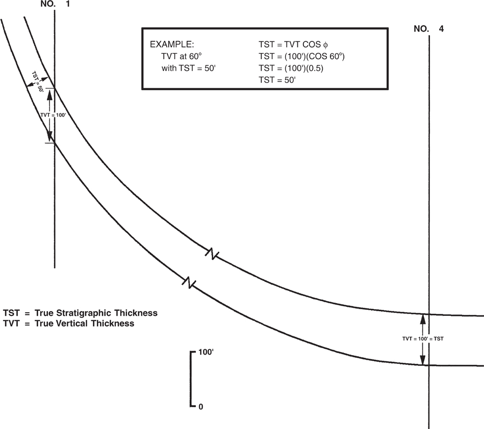
Figure 4-14 The cross section shows the effect of changing bed dip on the true vertical thickness of a stratigraphic section.
These examples show that log thickness in vertical wells varies with changes in structural dip and is equal to the TST only when the dip of the unit is zero (Fig. 4-14, Well No. 4). They also emphasize that log correlation is not an isolated process. Structural and stratigraphic relationships and geological knowledge of the area of study must always be kept in mind during correlation. Errors in correlation and incorrect assumptions on such aspects as the local growth history of a structure may be incorporated into the geological work. Such pitfalls can be prevented if the structural and stratigraphic framework of the area is considered during correlation.
Electric Log Correlation—Directionally Drilled Wells
In this portion of the chapter we discuss fundamental concepts and techniques for correlating directionally drilled wells. Additional complexities in correlation arise when working with logs from wells deviated from the vertical. We also look at the correlation of vertical wells with directionally drilled wells (often referred to as deviated wells).
What is a directionally drilled well? We discussed earlier that a vertical well is one drilled 90 deg to the horizontal reference, usually sea level. A directionally drilled well can be defined as a well drilled at an angle less than 90 deg to the horizontal reference, as shown in Figure 4-15. Some general directional well terminology was discussed in Chapter 3. These terms are again illustrated in Figure 4-15 for ease of reference. Other terminology discussed earlier in this chapter for vertical wells is also applicable to deviated wells.

Figure 4-15 Diagrammatic cross sections illustrating (a) a simple ramp or L-shaped well; (b) a more complicated S-shaped well; (c) a horizontal well. [(a) and (b) published by permission of Tenneco Oil Company; (c) published by permission of J. Brewton.]
Most wells drilled in an offshore environment and many wells onshore are drilled directionally. The most common well is a simple ramp well (Fig. 4-15a), sometimes called an L-shaped hole. These wells are deviated to a certain angle, which is usually held constant to TD of the well. Many wells are drilled with an S-shaped design. With an S-shaped hole, the well builds to one angle, maintains this angle to a designated depth, and then the angle is lowered again, often going back to vertical (Fig. 4-15b). Today we see a large number of horizontal wells, which are shaped by continually building the angle until the desired near-horizontal orientation is reached (Fig. 4-15c). By 2018, almost 90% of the wells being drilled in the United States were classified as horizontal wells, and another 5% were classified as deviated wells according to the weekly Baker Hughes rig count.
Log Correlation Plan
Just as with vertical wells, there must be some system to log correlation of directionally drilled wells. Due to the nature of deviated wells, a good correlation plan is critical to accurate correlations. For this log correlation plan, we once again use the structure map on the 8000-ft Sand on a normally faulted anticlinal structure (Fig. 4-16). The correlation plan outlined here is intended to make correlation systematic, provide a logical method for correlating directionally drilled wells with other directionally drilled wells or with vertical wells, and reduce correlation problems.
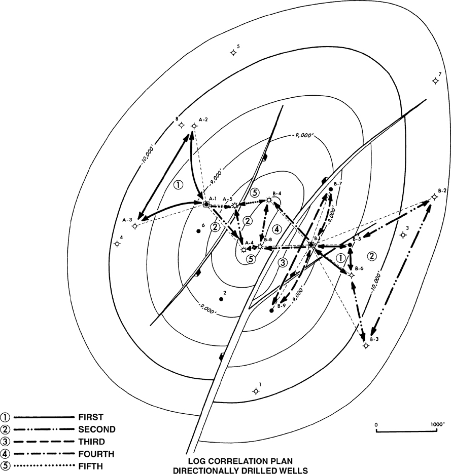
Figure 4-16 An example of a log correlation plan for directionally drilled wells. The plan shows the hierarchy of the log correlation sequence and illustrates how to correlate deviated wells in closed loops.
Step 1. Construct a correlation type log. Refer to the section on correlation type logs for the complete definition of a type log. Do not use a deviated well in the construction of a type log because a log from a directionally drilled well does not represent the true vertical stratigraphic section. Wells farthest off structure serve as good type log candidates. If no vertical wells are available for the correlation type log, a TVD log from a deviated well drilled in an area of low bed dip may be an acceptable substitute.
Step 2. Correlate all the vertical wells before correlating the deviated wells, since the vertical wells are usually easier to correlate. For the vertical wells, use the same plan outlined in Figure 4-7.
Step 3. Once the vertical wells have been correlated, begin correlating the deviated wells. To begin directional well log correlation, first organize the wells according to their direction of deviation with respect to structural strike. Deviated wells are classified into one of three groups: (1) wells drilled down-dip, (2) wells drilled along strike, and (3) wells drilled up-dip.
Step 4. Begin correlation of these three groups with the wells drilled generally down-dip. First correlate the wells with the least amount of deviation, and where possible, correlate in closed loops with each well log correlated with a minimum of two other wells. The wells with the least amount of deviation will have a log section thickness closer to that seen in a vertical well than other wells drilled down-dip. Looking at the wells drilled from Platform B in Figure 4-16, the first directional wells correlated are those represented by a billiard ball type correlation sequence number 1. There are two wells drilled with a minimum down-dip deviation (Wells No. B-5 and B-6). These wells can be correlated to each other and then with the straight hole, Well No. B-1, drilled as a vertical well from the platform.
Step 5. Continue correlating wells with increased deviation in the down-dip direction. For this example, these are Wells No. B-2 and B-3, indicated by correlation sequence number 2. These two highly deviated wells can be correlated with each other and then with Wells No. B-5 and B-6. Also, the vertical Well No. 3 may be used to correlate B-2 and B-3, since it is an off-structure well exhibiting a thick stratigraphic section.
Step 6. When all wells classified as being deviated down-dip are correlated, the next group to correlate are those wells deviated along structural strike. From Platform B, Wells No. B-7 and B-9 fall into this category. These wells can be correlated to each other and then with straight hole B-1 to close the loop. When correlating wells drilled along strike, the effect of wellbore deviation can be removed from the representative thickness of the directionally drilled wells by using a TVD log. In other words, the TVD log of a well drilled along strike will be similar to a vertical well drilled in the same dip location. The TVD log will still be affected by any true stratigraphic variations as well as apparent stratigraphic variations due to bed dip. Using a TVD log of a well drilled along strike can often simplify correlation.
Step 7. Correlate the wells deviated up-dip. Those wells drilled closest to the crest of the structure usually are complicated by stratigraphic thinning, faulting, and unconformities. The correlation of these wells can be most difficult; therefore, they are normally correlated last when all other correlation information is available and you can recognize the best correlation markers. Wells No. B-4 and B-8 drilled from the B Platform fall into this category. They are labeled as correlation sequence number 4. Wells drilled in an up-dip direction can have variable log section thickness due to the geometric relationship between a wellbore and structural dip. A log section from a well drilled in an up-dip direction can be thicker, thinner, or equal to the thickness of a log section from a nearby vertical well drilled through the same stratigraphic section. This potential complexity can add to the difficulty of correlating wells drilled in an up-dip direction. Because of these complexities, we recommend that these wells be correlated last, after significant knowledge is gained from other correlation work.
Step 8. Generally, it is best to correlate wells located nearest each other, especially in areas where significant changes in stratigraphic thickness are probable. Wells nearest each other and approximately in the same structural position usually are expected to have the most comparable interval thicknesses.
Step 9. After correlating the wells from one platform, begin correlation of wells on any additional platforms in the area. In Figure 4-16, the A Platform wells in the northwest portion of the field should be correlated next. It is not necessary, however, to isolate correlation to a single platform. Often, wells from one platform are drilled in a direction toward another platform. If wells from separate platforms are in close proximity to one another, they should be correlated to each other. Notice that correlation sequence number 5 illustrates the correlation of B-4 with A-5, and B-8 with A-4. Wells No. A-1 and B-1 are straight holes drilled from separate platforms, but since they are located in a similar structural position, they can also be correlated to each other.
The primary focus of this correlation plan is to provide a logical method for correlating all vertical and deviated wells in an area of study. The plan outlined is by no means the only one that can be used. The important point is to have a plan. Without one, log correlation becomes a random process, often resulting in some type of correlation problem or in miscorrelations.
Correlation of Vertical and Directionally Drilled Wells
In this section, we discuss general procedures for correlating vertical wells with directionally drilled wells. Directional wells have a measured log thickness (MLT) that can be less than, greater than, or equal to the log thickness in a vertical well drilled through the same stratigraphic section. These different MLTs result in additional complexities that must be considered when undertaking correlation work using well logs from both vertical and deviated wells.
Now we look at the correlation of a vertical well with a deviated well. Figure 4-17 shows a portion of an electric log from vertical Well No. A-1 and the electric log from directionally drilled Well No. A-2. The wells are in close proximity to each other. The detailed electric log correlation (sand and shale sections) for both wells indicates that they have penetrated the same stratigraphic section. Although both wells have a high degree of correlation (see SRM 1 through SRM 4), the stratigraphic section in Well No. A-2 is much thicker than the same section seen in Well No. A-1. The log section in Well No. A-1 from SRM 1 to SRM 4 is 490 ft thick. The same section in Well No. A-2 is 735 ft. Earlier in the chapter, in the discussion on vertical wells, we mentioned that a short section in one well with respect to another might be the result of stratigraphic changes or a fault. If the short section is isolated to one particular location, the short section is most likely the result of a fault rather than variations in stratigraphy. Conversely, if the short section is uniformly distributed over a series of intervals, the short section is probably due to stratigraphic variations rather than a fault.

Figure 4-17 Portion of an electric log from a vertical well (A-1) and a directionally drilled well (A-2). The electric log sections show detailed correlations.
Based on correlation criteria, the thinner section in Well No. A-1 appears to be the result of stratigraphic thinning rather than a fault. In this example, however, we introduce another possible explanation for the shortening. Since Well No. A-2 is directionally drilled, the thickness seen in the well with respect to Well No. A-1 may be completely the result of the wellbore deviation. Figure 4-18 shows vertical Well No. A-1 and deviated Well No. A-2 in its true orientation with respect to the vertical. Well No. A-2 is drilled due west at a deviation angle of 48 deg (from the vertical). The correlation markers in each well show that the strata are horizontal, and the thick section seen in Well No. A-2 is solely the result of wellbore deviation. We have now introduced another complexity in correlation that must be considered when both vertical and deviated wells are present in the area of study.
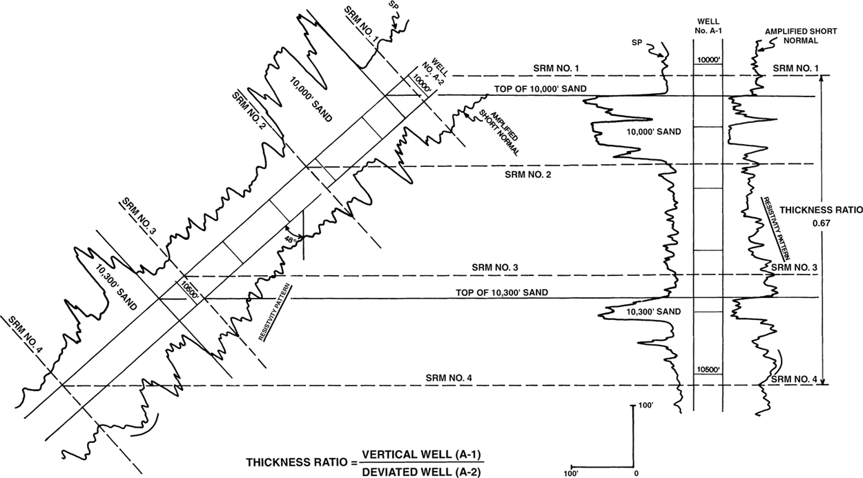
Figure 4-18 Vertical Well No. A-1 and deviated Well No. A-2 (shown in its true orientation with respect to vertical). The correlation markers show that the thicker section in Well No. A-2 is a direct result of its deviation from the vertical.
Here are several procedures that can be used to help correlate a vertical well with a directionally drilled well.
Mark the angle of deviation for the directional well on the log at least every 1000 ft. This provides a reminder that the well is deviated and indicates the angle of deviation at 1000-ft intervals on the actual log.
To compare interval thicknesses, slide the vertical well log as you correlate from marker to marker. This allows you to compensate during correlation for the expanded or reduced section in the directional well as a result of its deviation.
Calculate a thickness ratio for certain correlation intervals of interest to help evaluate whether any short section is the result of faulting, stratigraphic thinning, or just wellbore deviation (Fig. 4-18).
If a copy machine with a reduction mode is available, calculate the correction factor required to convert the deviated (stretched) log section to a vertical log section, and then reduce the log by the appropriate reduction factor. Use the reduced log for correlation.
In areas of horizontal beds or low relief, the MD log from a deviated well can be corrected for wellbore deviation and converted into a TVD log to use for correlation.
In areas with bed dips greater than 5 deg to 10 deg, if dip data are available from a dipmeter log or previously constructed structure maps, these data can be used to convert the deviated log to a TVT log. A TVT log is one in which the measured thickness has been corrected for wellbore deviation and bed dip to the thickness represented in a vertical well. In areas of significant dip, a TVD log provides little aid, if any, in correlation and can actually cause correlation problems (see section on MLT, TVDT, TVT, and TST) unless the well is drilled along the strike of the beds.
Estimating the Missing Section for Normal Faults
Earlier in this chapter, we discussed the procedure for estimating the depth and missing section for a fault in a vertical well by correlation with another vertical well. Now we present the method for estimating the depth and missing section for a fault when deviated wells are considered. First, we look at the situation involving an area with horizontal beds.
Horizontal Beds.
We begin with a fault in the deviated Well No. A-2 (Fig. 4-19a). By correlation with vertical Well No. A-1, this well cuts a fault near the 10,000-ft Sand level. To determine the depth and missing section, we correlate the logs in the same manner as previously outlined in this chapter. First, correlate down the logs starting with SRM 1. We can say that correlation is lost at points A in both wells. Mark this location on the two logs. Next, find a correlation point below this section on the logs, such as SRM 4, and correlate up the logs. We now lose correlation in the wells at points B. By detailed correlation of the shale markers and sands, we have determined that Well No. A-2 is faulted, and the section in Well No. A-1 that is stratigraphically equivalent to the missing section in Well No. A-2 is highlighted in Figure 4-19a–b.
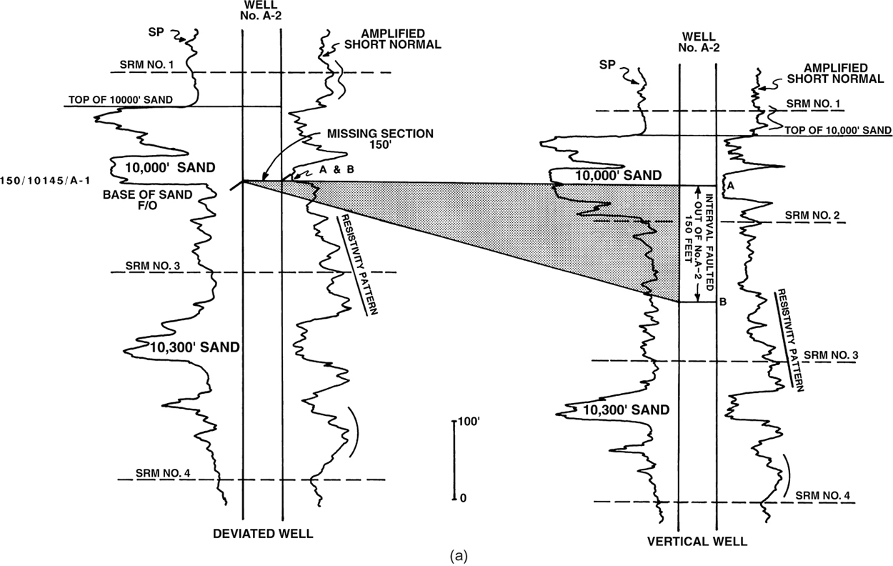
Figure 4-19(a) Detailed correlation of a deviated well with a vertical well to locate the depth and the missing section for a fault in the deviated well. The base of the 10,000-ft Sand is faulted out.
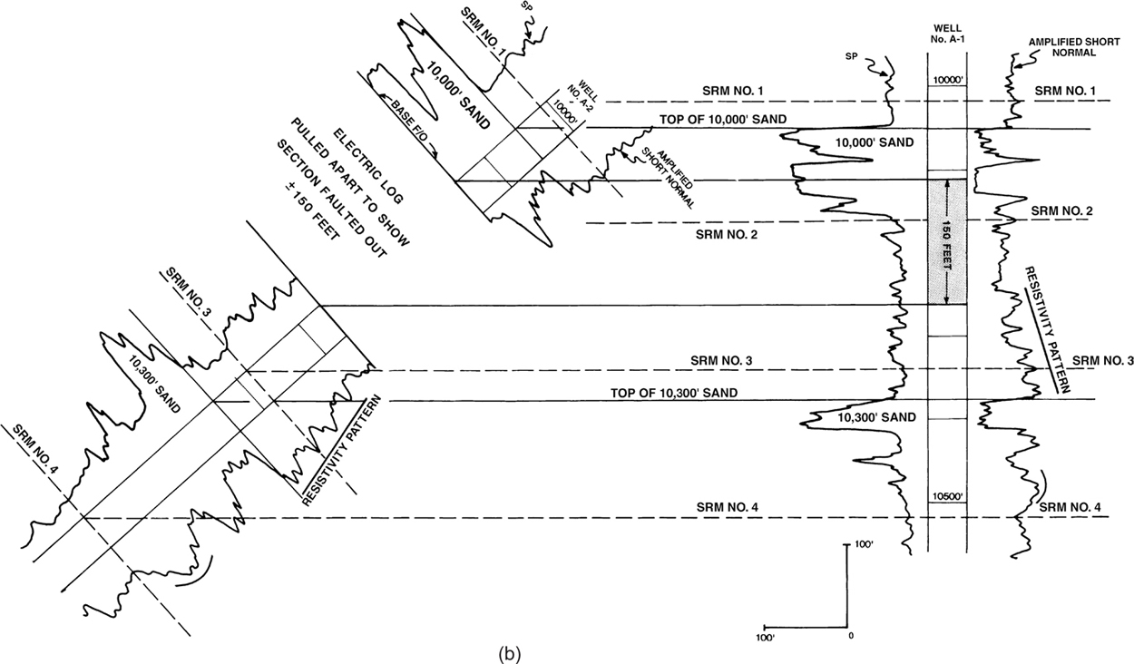
Figure 4-19(b) The simplified stratigraphic section through Wells No. A-1 and A-2 illustrates that the missing section in Well No. A-2 is equivalent to the vertical section highlighted in Well No. A-1. No thickness correction factor is required in this example.
The faulted out or missing section in Well No. A-2 is equal to 150 ft by correlation with Well No. A-1. Notice that the base of the 10,000-ft Sand is faulted out of Well No. A-2. This information is annotated on the log along with the amount of missing section, the depth of the fault, and the well(s) used to correlate the fault.
The missing section in directional Well No. A-2 is determined by correlation with Well No. A-1, which is a vertical well. In a vertical well, the measured log thickness and vertical thickness are the same. Since missing section is expressed as the vertical thickness of the stratigraphic interval faulted out of a well, the vertical thickness of the missing section in Well No. A-2 is 150 ft. The 150 ft represents the missing section for the fault. This information will be used in future fault and structure mapping.
Figure 4-19b is a simplified stratigraphic section showing Wells No. A-1 and A-2 positioned in their true orientation with respect to the vertical. Well No. A-2, which is deviated at 48 deg from the vertical, is pulled apart at the fault to show the restoration of the faulted-out section. This cross section clearly illustrates that the missing section in Well No. A-2 is equal to the 150 ft of vertical section highlighted in Well No. A-1.
Now consider a fault in vertical Well No. A-1 correlated with deviated Well No. A-2 (Fig. 4-20a). Well No. A-1 has a fault near the base of the 10,000-ft Sand. Detailed correlation, as shown in the figure, identifies a 225-ft section in deviated Well No. A-2 that is faulted out of Well No. A-1. The faulted-out section is highlighted in the figure. Since the missing section for the fault is determined as the TVT of the stratigraphic interval faulted out of the well, the estimate of 225 ft of missing section based on the deviated log thickness must be corrected to express the missing section in terms of TVT.
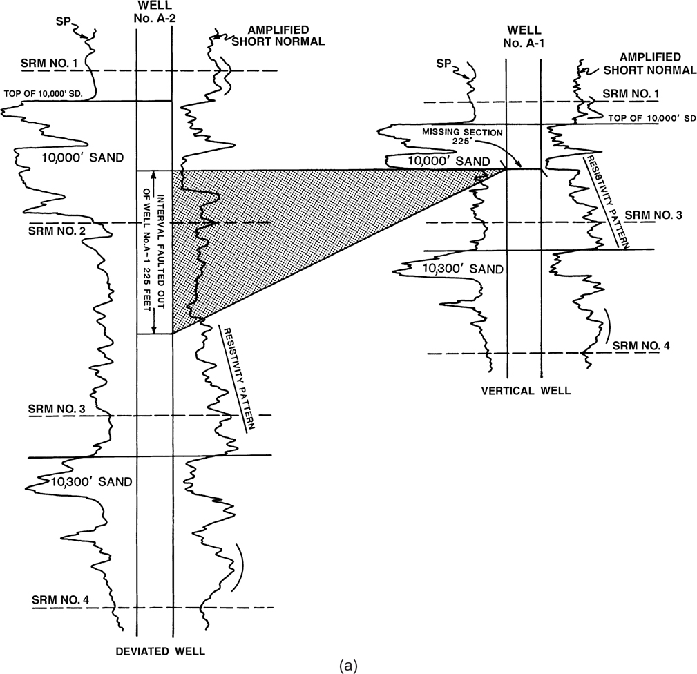
Figure 4-20(a) Detailed correlation of a vertical well with a deviated well to locate the depth and determine the missing section for a fault in the vertical well.
Figure 4-20b is a stratigraphic section showing Wells No. A-1 and A-2 positioned in their true orientation relative to vertical. The log section of Well No. A-1 is pulled apart at the fault to show the restoration of the faulted out section. Since we are working in an area with horizontal beds, the correction of the measured log thickness in Well No. A-2 to TVT is determined by the simple trigonometric solution of a right triangle. The insert in the center of the figure shows that the TVT of the missing section is equivalent to the vertical side of a right triangle whose hypotenuse is equal to the log thickness of the missing section in deviated Well No. A-2.
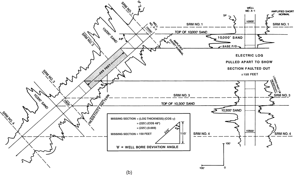
Figure 4-20(b) A simplified stratigraphic section illustrating the relationship of the missing section in vertical Well No. A-1 to the exaggerated sections seen in deviated Well No. A-2. The exaggerated section in Well No. A-2 must be corrected for wellbore deviation to determine the true amount of missing section.
Where

Therefore,
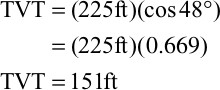
The actual (corrected) missing section for the fault in Well A-1 determined by correlation with deviated Well No. A-2 is 150 ft.
Dipping Beds.
The procedure for correlating deviated wells in an area of significant dip is, in effect, the same as that presented thus far in this chapter. The primary difference occurs in estimating the actual missing section resulting from a normal fault. Since the missing section due to a fault is defined as the TVT of the stratigraphic interval faulted out of a well, any missing section value determined by correlation with a deviated well exhibiting a measured log thickness must be converted to TVT. In the previous section, we defined a simple trigonometric relationship for calculating the correction factor applicable in areas with horizontal beds. Where dipping beds are present, the mathematical correction factor becomes somewhat more complex.
There are several equations available for calculating a correction factor to convert MLT in a deviated well to TVT. We present two methods for computing the correction factor.
Method 1—Two-Dimensional Correction Factor.
For the 2D correction factor, there are two correction factor equations, assuming that the well is drilled at a constant inclination and azimuth over the interval in question. The first, called Type 1, is used where a deviated well is drilled in a direction that is general opposite to that of the bed dip. In other words, the well is deviated in the up-dip direction (Fig. 4-21a). The bed dip would be an apparent dip in most cases. The second, called Type 2, is used where a deviated well is drilled in the same general direction as that of the bed dip; the well is deviated in the down-dip direction (Fig. 4-21a). Again, the bed dip is typically apparent dip.
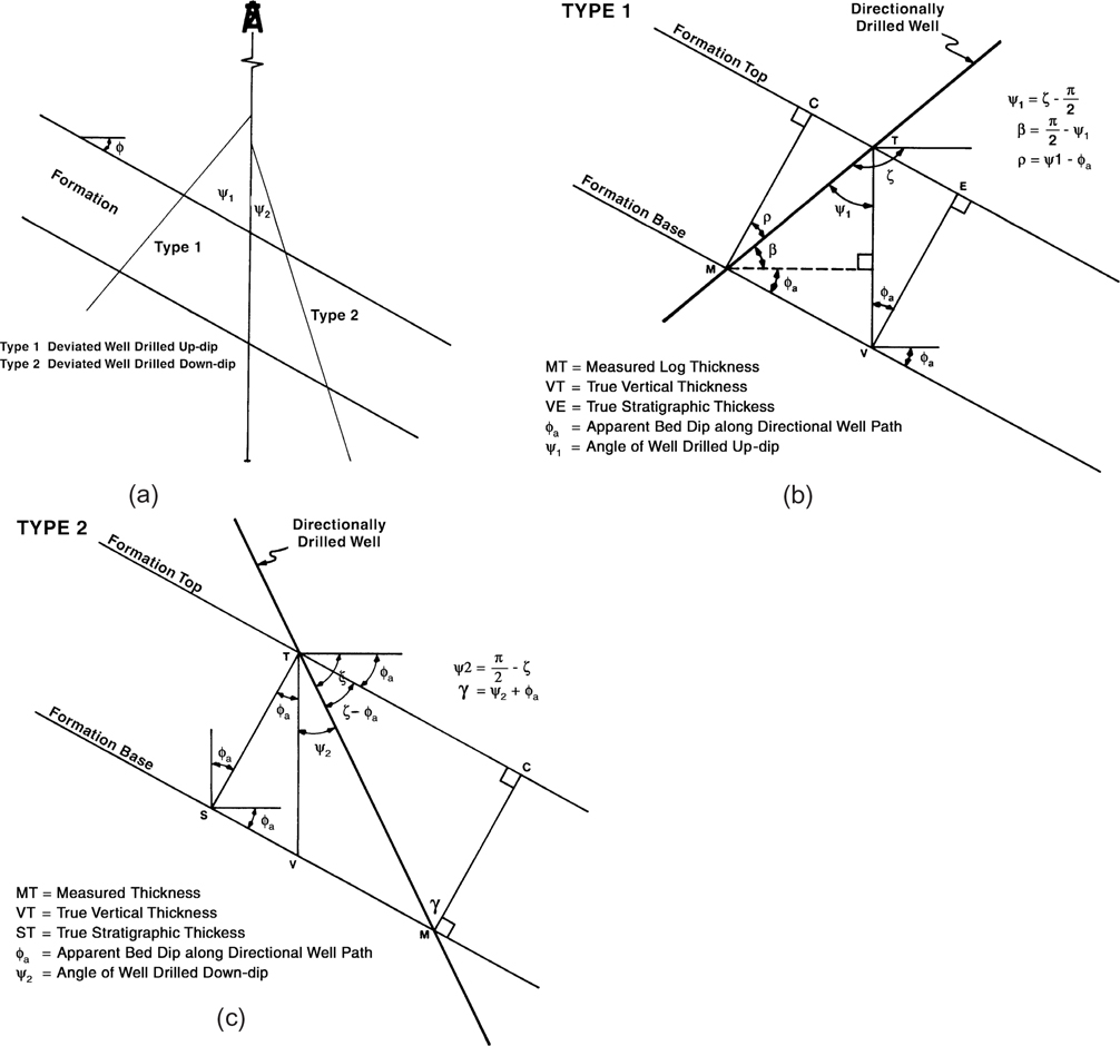
Figure 4-21 (a) Cross section illustrating the formation/wellbore deviation relationship for the Type 1 and 2 correction factors. (b) The cross section shows the detailed wellbore/formation geometry used to derive the Type 1 correction factor. (c) The cross section shows the detailed wellbore/formation geometry used to derive the Type 2 correction factor. (Published by permission of D. Tearpock and R. Bischke.)
Type 1 Equation. The derivation of the Type 1 equation (well deviated up-dip) is shown here and illustrated in Figure 4-21b.
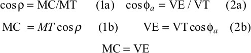
Therefore, equating 1b and 2b,
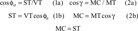
Rearranging,
Substituting ρ = ψ − ϕa and relabeling VT as TVT, and MT as MLT,

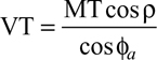
Type 2 Equation. The derivation of Type 2 (well deviated down-dip) is shown here and illustrated in Figure 4-21c.
Therefore, using 1b and 2b and relabeling VT as TVT, and MT as MLT,
Rearranging,

Substituting γ = ψ2 + ϕa

With Eqs. (4-4) or (4-5), the data required to calculate the correction factor are (1) ϕa = wellbore deviation from the vertical, (2) ϕa = apparent bed dip (bed dip in the direction of wellbore deviation), and (3) MLT = measured log thickness in the deviated well. The apparent bed dip is the most difficult data to obtain for these equations. The only source of apparent bed dip is from an existing structure map. If an existing structure map is available the apparent bed dip along the well path can easily be calculated using the rise/run equation discussed in Chapter 2 (Eq. 2-2).
Method 2—Three-Dimensional Correction Factor.
In this section, we present an exact 3D correction factor equation. A version of the equation was first presented by J. Setchell (1958) and has been used successfully for more than 60 years. We consider this 3D correction factor equation preferable because this equation can be used to calculate the correction factor regardless of the direction of wellbore deviation, and the true dip of the beds is used instead of the apparent dip, which is used in the 2D equations.
To derive the general 3D equation, we introduce a 3D spherical coordinate system (Fig. 4-22) with one horizontal axis in the direction of dip (called the x-axis), one axis perpendicular to the first and also horizontal (called the y-axis), and one axis perpendicular to the other two (called the z-axis). In this equation we assume that the well is straight within the interval of interest (i.e., the well has both a constant deviation and azimuth over this interval). If the well has a significant change in deviation and/or azimuth over the bed of interest, you can calculate the straight-line distance, inclination and azimuth from the point of entry into a unit to the point of exit from the unit and use these values in Eq. (4.6) rather than measured log thickness and information from the well directional survey. We also assume that the top and base of the bed are parallel to one another. The case where the top and the base of the bed is not parallel is discussed in Chapter 14. The origin is the point (T) at which the wellbore first penetrates the bed.
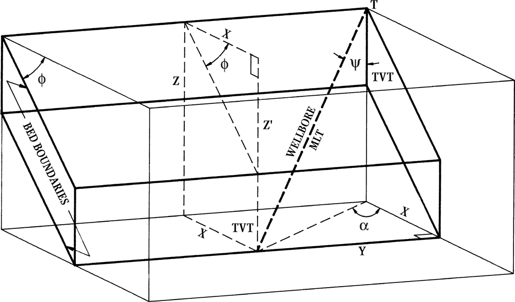
Figure 4-22 A 3D spherical coordinate system with one horizontal axis in the direction of bed dip (x-axis), one axis perpendicular to the first and also horizontal (y-axis), and one axis perpendicular to the other two (z-axis). (Published by permission of D. Tearpock.)
Where

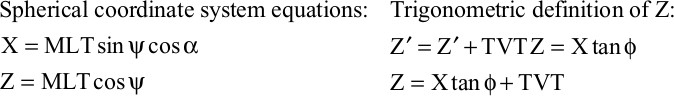
Substituting the spherical coordinate definition for Z, X, and the alternate trigonometric definition of Z easily yields Eq. (4-6).
Application of Methods 1 and 2.
Now apply these methods using the data shown in Figure 4-23. Wells No. A-1, A-2, and A-3 are drilled from a single location and penetrate a section that includes Bed A, which is of constant thickness and dips at 35 deg due east. Well No. A-1, a vertical well, cuts a fault that completely faults out Bed A. Well No. A-2 is drilled in a down-dip direction with an average deviation angle of 36 deg through Bed A. Well No. A-3 is drilled directly up-dip with a deviation angle of 35 deg through Bed A. For simplicity, the wells are all assumed to be drilled in a vertical plane parallel to the dip of Bed A.
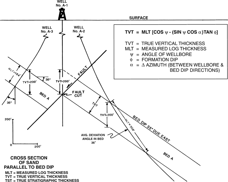
Figure 4-23 One vertical and two deviated wells penetrate Bed A. In Well No. A-1, Bed A is faulted out. The cross section shows the relationship of the missing section in Well No. A-1 to the MLT of the equivalent interval in deviated Wells No. A-2 and A-3. The equation shown is used to correct MLT to TVT.
Through detailed correlation of the three wells, a fault is identified in Well No. A-1. Based on the correlations, Bed A is completely faulted out of the well. Assuming that Wells No. A-2 and A-3 are the only wells available for correlation, the amount of missing section for the fault in Well No. A-1 must be estimated from these deviated wells.
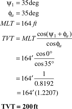
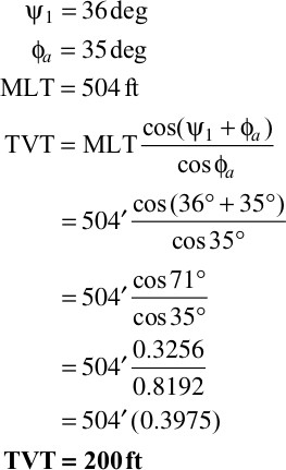
Considering again that missing section is defined as the true vertical thickness of the stratigraphic interval faulted out of a well, and the fault in Well No. A-1 completely faults out Bed A, the missing section resulting from the fault in Well No. A-1 is equal to the true vertical thickness of Bed A. A review of Figure 4-23 shows that Bed A has a true vertical thickness of 200 ft. When we correlate Well No. A-1 with the two deviated wells, however, we obtain a missing section in terms of deviated log thickness rather than true vertical thickness. Therefore, these deviated log thicknesses must be converted to true vertical thickness to estimate the amount of missing section. The missing section (Bed A) in Well No. A-1 has a logged thickness in Well No. A-2 of 504 ft Zand a logged thickness in Well No. A-3 of 164 ft. The logged thickness of 504 ft in Well No. A-2 is over two and one-half times greater than the TVT. The logged thickness of 164 ft in Well No. A-3 is less than the TVT (0.82).
By log correlation, the amount of missing section for the fault in Well No. A-1 ranges from 164 ft, based on correlation with Well No. A-3, to 504 ft, by correlation with Well No. A-2. What is the actual missing section for the fault? In order to determine the actual missing section, the log thickness measured in Wells No. A-2 and A-3 must be corrected to true vertical thickness.
TVT Calculation Using Method 1
Type 1: Well Drilled Up-Dip. In order to use Eq. (4-4) to calculate the correction factor, three pieces of data are required: (1) the wellbore deviation angle (ψ1), which can be obtained from the directional survey of Well No. A-3, (2) the formation dip (ϕa), which is true dip in this case, obtained from a dip meter log or a completed structure map, and (3) the MLT in Well No. A-3 that is equivalent to the section missing in Well A-1.
Data:
Type 2: Well Drilled Down-Dip. In order to use Eq. (4-5), the same parameters used in Eq. (4-4) are required.
Data:
Since Wells No. A-2 and A-3 are drilled directly down-dip and up-dip respectively, the value for bed dip in Eqs. (4-4) and (4-5) is equal to the true bed dip (f). This can be obtained from a structure map or a dipmeter if available. If the direction of wellbore deviation is not parallel to bed dip, however, then an apparent bed dip in the direction of wellbore deviation must be determined. This apparent bed dip cannot come from a dipmeter log because this log calculates true bed dip. This is one of the main drawbacks to the 2D equations. Apparent bed dip can be derived from a structure map by using Eq. 2-2 where rise/run is measured along the path of the deviated well and not perpendicular to bed strike.
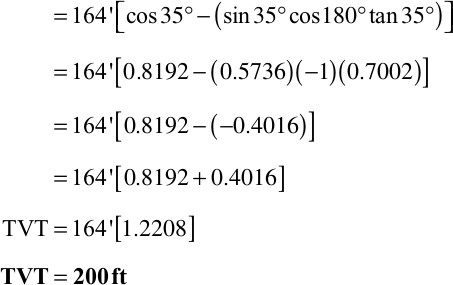
TVT Calculation Using Method 2 The required data to solve the general 3D equation are (1) wellbore deviation angle (ψ) obtained from a directional survey, (2) wellbore deviation azimuth (αw) obtained from a directional survey, (3) true bed dip (ϕ) measured from a completed structure map or dipmeter if run in the wellbore, (4) bed dip azimuth (αa) measured from a completed structure map or obtained from a dipmeter, and (5) MLT that is equivalent to the missing section. TVT for Well No. A-2:
Data:
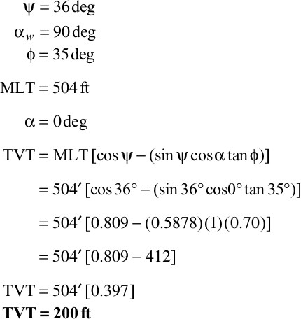
TVT for Well No. A-3: The data for this calculation are exactly the same as for Well No. A-2, with two exceptions. The azimuth (αw) for Well No. A-3 is due west, or 270 deg, and therefore the ∆ azimuth (α) is 180 deg and ψ is 35 deg.
Through the use of the 2D and 3D equations, we have successfully calculated the amount of missing section for the fault in Well No. A-1. Notice the close agreement between the different equations. The missing section estimated at 200 ft can now be used for all future fault surface mapping and structure map integration as well as other geological work, such as cross-fault drainage analysis. The actual procedure for integrating a fault and structure map is detailed in Chapter 8. We have now defined two methods for obtaining the correct values for missing section when correlating with deviated wells. Anytime you are correlating in an area with deviated wells and dipping beds, missing and repeated section are defined in terms of TVT. Significant errors in structure maps, net pay maps, and even proposed well locations can occur if these corrections are not made or if missing section is not understood in terms of vertical separation (see Chapter 7).
MLT, TVDT, TVT, AND TST
The thickness of any given interval on a log is referred to as the measured log thickness (MLT). In a vertical well, the MLT for any given interval is equal to the TVT of the interval. We know from the previous discussion in this chapter, however, that the MLT in a directionally drilled well is normally not equal to TVT because of the wellbore deviation and to bed dip in areas of dipping beds. However, remember that MLT will approximate TVT in the near-vertical part(s) of a directional well.
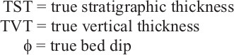
True vertical depth thickness (TVDT) is defined as the MLT between two specific points in a deviated well, corrected only for wellbore deviation. The true vertical thickness (TVT) is defined as the thickness of an interval measured in the vertical direction. It is the thickness seen in a vertical well. For a directionally drilled well, the TVT can be calculated using the equations introduced in the previous section. The true stratigraphic thickness (TST) is defined as the thickness of a given interval measured at a right angle to the bedding surface in a vertical cross section. It can be calculated by multiplying the TVT by the cosine of bed dip.
These various thicknesses are graphically illustrated in Figure 4-24. In Figure 4-24a, a well deviated up-dip at an angle of 50 deg penetrates strata dipping 35 deg due west. The MLT of the strata is 127 ft. To correct the MLT to TVDT, the MLT (127 ft) is multiplied by the cosine of the wellbore deviation angle (50 deg). The resultant TVDT is 82 ft.

Figure 4-24 (a) The MLT in a well deviated up-dip is compared to TVDT, TVT, and TST. (b) The MLT in a well deviated down-dip is compared to TVDT, TVT, and TST. (c) The TVDT, TVT, and TST calculated from a deviated well have the same value when the beds are horizontal.
Figure 4-24b shows the same strata penetrated by a well drilled down-dip at an angle of 40 deg. The MLT of the strata in the well is 476 ft. Corrected to TVDT, it is 357 ft. The correction factor equations developed in the previous section are used to calculate a TVT of 150 ft for the penetrated strata in Figure 4-24b. The TST of the strata calculated by multiplying the TVT (150 ft) by the cosine of the bed dip (35 deg) is 123 ft.
Notice that for the well drilled down-dip, the MLT is 3.17 times greater than the TVT, and the TVDT is 2.38 times greater than the TVT. For the well drilled up-dip, the MLT is less than the TVT, and the TVDT is about one-half the TVT.
The understanding of these various measurements is very important in log correlation and the determination of the value for the missing section. Very often, when a well is directionally drilled, a TVD log is automatically prepared as part of the logging program. The TVD log is then used to aid in correlation, determine missing or repeated section resulting from a fault, and count net sand and net pay. Figure 4-24 illustrates that in areas of significant dip, a TVD log of a well not drilled along strike may provide little, if any, advantage over the deviated well log for correlation and can actually complicate the estimation of missing section. Observe in Figure 4-24b that the TVDT, which is the thickness seen in a TVD log, is still 2.38 times greater than the TVT.
Consider a fault in this section (Fig. 4-24b) that exactly faults the entire unit out of the well. The amount of missing section in that well would be 150 ft. By correlation with the well deviated down-dip, the missing section would be estimated to be 476 ft; with a TVD log, the estimated missing section for the fault would be 357 ft. We can conclude that the TVD log could provide a considerable error in the estimation of the amount of missing section. If the data are available, we recommend that a TVT log be prepared. This log can be used to aid in correlation and to estimate the amount of missing section due to a fault, since it represents the TVT of the interval logged.
The preparation of a TVD log for the well deviated up-dip in Figure 4-24a could actually result in additional correlation problems. Notice that the measured thickness of the strata in the deviated well is 127 ft. Converting this MLT to a TVD log thickness actually reduces the thickness of the interval to 82 ft. This reduced thickness could be mistakenly interpreted as stratigraphic thinning. If the TVD log were used to estimate the missing section for the fault, it would result in an underestimate. For example, if we again use a fault in this section with a missing section of 150 ft, then by correlation with a TVD log for the well drilled up-dip, the missing section for the fault would be estimated at 82 ft, or nearly one-half the actual size.
In areas of horizontal or nearly horizontal beds, TVDT is equal to or nearly equal to TVT (Fig. 4-24c) and can be of significant help in correlation and estimating the value for missing section. In areas of dipping beds, however, a TVD log may provide little help and can actually cause additional correlation problems that may result in mapping errors.
Electric Log Correlation—Horizontal Wells
Horizontal wells require some additional techniques in log correlation. Ordinary methods for correlating deviated wells can be used before the wellbore reaches an angle close to the bed dip angle. However, where the borehole angle is very close to the bed dip, the log curves are extremely stretched compared to a vertical well log. Also, the response of the logging tool is affected by its eccentric position in the borehole and lack of symmetry of the beds around the borehole. In vertical wells a logging tool is more or less in the center of the hole and the bed boundaries are near horizontal or at some reasonable angle to the borehole, so the tool is reading the same lithology around the borehole at a given depth. In horizontal boreholes the bed boundaries are nearly parallel to the borehole, so it is possible to have sand on one side of the hole and shale on the other. The tool would then be reading some averaged value for the two lithologies. Next, we briefly discuss some of the basic methods of recognizing bed boundaries and correlating horizontal wells.
Direct Detection of Bed Boundaries
When a logging tool crosses a bed boundary, there is some change in the value recorded on the log. In vertical wells this change is fairly abrupt, so specific log curve shapes can be matched from well to well. In horizontal wells these curve shapes are stretched out due to the low angle between borehole and bed boundary. For example, a gamma ray curve might change from indicating shale to indicating sand within a foot or two in a vertical well; but in a horizontal well this change may be stretched out over tens of feet or more as the borehole gradually crosses from shale into sand. Although the gamma ray log is directly indicating the bed boundary, the stretched curve may be difficult to correlate without rescaling or shrinking its length. We discuss methods for doing this in the sections on TVD and TSD methods.
Electromagnetic propagation resistivity logging tools, such as those used in logging-while-drilling (LWD) systems, record spikes on the log curve at boundaries where significant changes in resistivity occur. Sand-shale bed boundaries, limestone-shale bed boundaries, and hydrocarbon-water contacts are examples of where these spikes would occur. These types of boundaries would be directly detectable with this type of tool, and the spikes could be directly correlated to the equivalent boundary in a nearby vertical well. Fagin et al. (1991) give an example of recognizing an oil/water contact using this method, as well as modeling log response to the proximity of an oil/water contact before it is penetrated.
Modeling Log Response of Bed Boundaries and Fluid Contacts
Logging service companies can compute the response of their tools to model stratigraphic sections and proximity to fluid contacts for horizontal boreholes. Using a nearby vertical well for control, resistivities and thicknesses are assigned to the model section. The response of the tool to the vertical model is computed and compared to the actual log from the vertical well. If it is a good match, then a set of log curves are computed for multiple angles of penetration of the stratigraphic section (i.e., various apparent bed dip angles to the borehole orientation). These model curves are then compared to the log from a horizontal borehole. If a match is found, this correlation to the vertical well determines the position of the horizontal borehole in the stratigraphic section or its proximity to a fluid contact. Leake and Shray (1991) give an LWD example using the technique to maintain a horizontal well within a 40-ft sand. This approach is well illustrated by Amer et al. (2013).
True Vertical Depth Cross Section
The previous methods are widely used to recognize specific bed boundaries and fluid contacts. But how can a geologist correlate a long section of a horizontal well log to a log from a vertical well? The geologist can build a cross section to aid in making the correlations using a vertical section plot from the directional survey and a TVD log from the horizontal well. If the TVD of the horizontal borehole stays constant for long sections of the hole, a measured depth log may be used with the TVD and vertical section (through the wellbore from the surface location to total depth) for correlation points posted on the log. The cross section can help you determine whether your correlation picks are at least geometrically consistent. TVD logs have highly distorted thicknesses in horizontal wellbores, but if the target zone is thick and you have been able to correlate the log as it approaches horizontal, you may be able to recognize the target zone bed boundary. Typically, the gamma ray and resistivity logs are used for TVD log correlation. However, if multiple bed boundaries are crossed or the borehole goes in and out of the target zone, a satisfactory correlation of a TVD log is unlikely. A TVT log would more accurately represent the thickness seen in the vertical well with which you are correlating, but the correction factor or reduction in length can be extreme. Most computer-based log correlation software can construct and display a TVT log if the bed dip is known.
The TVD cross section can be constructed with standard cross-section methods and a few additional considerations.
Plot the vertical section of the well on cross-section paper with a suitable vertical exaggeration (e.g., 10:1).
Plot the bed boundaries for the part of the well as it approaches the horizontal segment of the well and estimate the vertical thickness to the top of the objective zone using a nearby vertical well. To determine the top of the objective zone, a pilot hole may be drilled vertically to the objective stratigraphic section before drilling the horizontal part of the hole.
Estimate the apparent bed dip in the plane of the cross section from maps, seismic data, or correlations among nearby vertical wells. Draw the bed boundaries on the cross section and try to pick the top of the objective zone where the projected top intersects the plotted borehole.
Adjust the dip of the bed boundary if your correlation indicates a different penetration point.
Continue projecting the beds and thicknesses along the cross section and look for correlations where the wellbore would be intersecting the plotted bed boundary. Note that if the wellbore goes up through a stratigraphic section, the log curve will be inverted (Fig. 4-25).

Figure 4-25 A gamma ray log in a wellbore that goes up stratigraphic section is upside down compared to a log from a vertical well. (From Tearpock 1999. Published by permission of Anadarko Petroleum Corporation.)
If the wellbore cuts a fault, use the TVT in the vertical well to estimate the missing section for the fault. That is, if your correlation shows the wellbore is 10 ft below the top of the target zone before crossing the fault and 20 ft above the top after crossing the fault, then the fault is a 30-ft fault. This is basically the estimated restored tops method described later in this chapter.
In general, the TVD cross section requires that bed boundaries are recognizable on a measured depth log recorded in the horizontal borehole or at least on the computed TVD log. Modeling of log response is often used to recognize the bed boundaries, and a cross section is constructed to illustrate the correlations. Singer (1992) gives an example of using modeling and illustrating the correlations with a cross section. Amer et al. (2013) also illustrate matching the LWD measurements in a horizontal well with modeled results from a nearby vertical well in order to correlate the horizontal well. This correlation work is most easily done on a computer.
True Stratigraphic Depth Method
Kyte et al. (1994) describe a method for correlating logs and building cross sections from horizontal wells. They call it the true stratigraphic depth, or TSD, method. Figure 4-26 illustrates the relationship of TVD, TVT, TST, and TSD. TVD is the actual vertical depth of a point in the wellbore or on the log. TSD is the stratigraphic position of a point in the wellbore or on the log. So any place on the same bed boundary would be considered to have the same TSD, and therefore, these points would correlate back to the same stratigraphic point in the vertical well. The idea is to use a computer program to rescale the log (usually the GR log) from the horizontal well for correlation with a nearby vertical well. One such program, developed by Union Pacific Resources Corporation, is called GRNAV. The technique uses the TVDs for a log from the horizontal well and an estimated change in TVD due to bed dip for the bed or correlation point. This allows an estimate of the stratigraphic position of a point on the log compared to a nearby vertical well. To make the correlation, a part of the log curve is rescaled based on this estimate and compared to the vertical well. The next segment along the wellbore is then correlated the same way until the whole log is correlated. In practice, the method is computer-based to correlate as the well is being drilled to provide real-time geological information for steering and maintaining the wellbore in the target zone.

Figure 4-26 A schematic vertical section along a horizontal wellbore with vertically exaggerated bed dip illustrating TVD, TVT, and TSD. Points in a wellbore that are in the same stratigraphic position have the same TSD. (From Tearpock 1999. Published by permission of Anadarko Petroleum Corporation.)
Figure 4-27 illustrates the method for determining the rescaled log length or thickness for correlating a stratigraphic interval between two points in a borehole going down section. TSD point 1 has already been correlated with the vertical well. TSD point 2 is a point in the wellbore selected by the interpreter. From TSD point 1, the bed dip is plotted and a ∆TVD for TSD point 1 is calculated at a point vertically above TSD point 2. Subtracting this ∆TVD value from the total TVD difference between the two TSD points leaves ∆TSD, which will be the rescaled log thickness of the horizontal well to use for correlation (Fig. 4-27). In the computer program a slider bar is used interactively to change the estimated dip and change the displayed log thickness. The log is then stretched or squeezed until the curve is matched to the vertical well to make the correlation. The program also generates a TVD cross section as correlations are made.
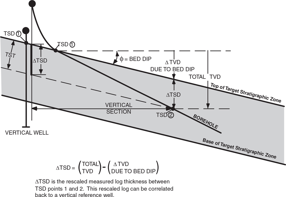
Figure 4-27 A schematic example of determining ∆TSD from TVD values to rescale a horizontal well log for correlation with a log from a vertical well. This example shows a wellbore or borehole going down section. (From Tearpock 1999. Published by permission of Anadarko Petroleum Corporation.)
Figure 4-28 illustrates the method for determining rescaled log thickness for a wellbore directed up section, which might occur if the wellbore extends too shallow relative to the target zone. A deeper horizon, such as the base of the target zone, is correlatable with the vertical well, and TSD point 2 is established and the apparent dip is drawn (Fig. 4-28). For the part of the wellbore going up section to the selected TSD point 3, the total TVD difference between TSD points 2 and 3 and the ∆TVD for TSD point 2 add to give ∆TSD. This vertical thickness will be the rescaled log thickness to use for correlations of the log section between TSD points 2 and 3. Of course, the log curve will also be inverted compared to the vertical well if the wellbore is deviated up stratigraphic section (Fig. 4-25). The GRNAV program can correct an inverted log curve.
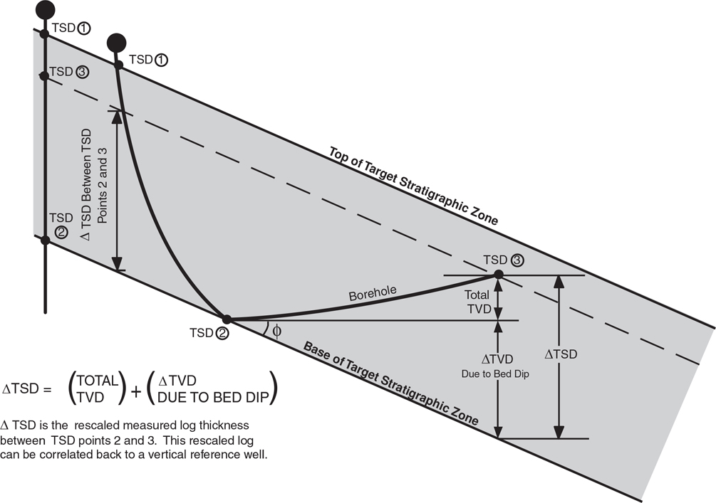
Figure 4-28 A schematic example of determining ∆TSD from TVD values to rescale a horizontal well log for correlation with a log from a vertical well. This example shows a wellbore or borehole going up section. (From Tearpock 1999. Published by permission of Anadarko Petroleum Corporation.)
Figure 4-29 is a generic illustration of the correlation of a horizontal well log and a vertical well log from Kyte et al. (1994). Figure 4-29a is a gamma ray log from a nearby vertical well or offset log with A, B, and C identifying three correlation markers. The wellbore geometry is shown in Figure 4-29b in a TVD cross section along the vertical section of the wellbore. A, B, and C are the bed boundaries identified by the correlation markers in the vertical well. The wellbore goes down stratigraphic section and up section with numbers indicating selected points illustrated in Figure 4-29e, the horizontal well log. Figures 4-29c and d are horizontal well log segments rescaled with the TSD method. The horizontal well log has been rescaled in Figure 4-29c from point 1 to point 3 in the horizontal well log, Figure 4-29e, to make the correlation to the vertical well. From point 3 on the horizontal well log to point 4, the log has been rescaled and inverted in Figure 4-29d, because the wellbore is going up section from points 3 to 4 (Fig. 4-29b).
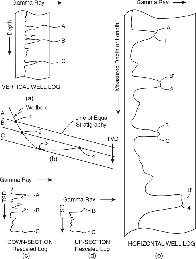
Figure 4-29 A generic illustration of the correlation of a horizontal well log with a vertical well log. (a) Vertical well log. (b) A TVD cross section drawn at true scale along the vertical section of the wellbore. Two gamma ray log curves have been rescaled from the horizontal well log for (c), a down-section part, and (d), an up-section part. (e) Horizontal well log. (From Kyte et al. 1994. Published by permission of Anadarko Petroleum Corporation.)
The TSD method is an effective way to rescale a log from a horizontal well with a computer program and correlate it to a nearby well. Good log character is required, and even with a gamma ray log, the response may be more gradual than in a vertical well due to the low angle at which the wellbore cuts across the bed boundary.
Computer-Based Log Correlation
As we have discussed so far in this chapter, paper-based log correlation techniques have been the basic tools utilized by geologists for more than 60 years. The transfer of these techniques onto the computer screen has resulted in significant advantages both in efficiency (i.e., saving time) and in the application of high-resolution stratigraphic analysis. This was shown in the previous section on horizontal well log correlation. Despite these promises, geologists were initially slow to migrate onto the computer. In this section of the chapter, we address the traditional problems geologists have encountered in their attempt to use the computer for log-correlation work, describe some of the solutions to these problems, and provide examples of the significant advantages gained from computer-based log correlation in subsurface interpretation.
Geologists often cite two significant reasons they cannot or will not work with well logs on the computer: (1) the lack of an inexpensive digital well log database, and (2) software tools that do not reflect geologists’ actual workflow with well logs. The digital-data availability issue is being actively addressed. Since the late 1990s, there has been a dramatic increase in the rate of well log digitization, including the advent of digital raster well log formats (Montgomery 1997a and b). The newly developed raster well log formats provide companies with an affordable option for accessing thousands of well logs for basin-wide studies. True digital log data is also becoming more widely available.
The second issue, that software tools did not reflect geologists’ workflow, has also been addressed with several new software offerings devoted to well log interpretation/correlation. The next section utilizes one of these new applications and addresses the specific tools and techniques necessary to transfer paper-based log-correlation techniques onto the computer screen.
Well Log Correlation: The Transition from Paper-Based to Screen-Based
Log correlation is a basic skill of the geologist, as discussed earlier in this chapter. A geologist uses this skill to perform the often-repeated tasks of picking correlation markers, formation tops, faults, and unconformities, along with net sand, porosity, and pay analysis. Advanced applications include electric log facies analysis and sequence stratigraphy. In the hands of an experienced geologist, these techniques can be used to correlate subtle stratigraphic features, faults, and unconformities with great accuracy over large distances.
In paper-based log correlation, we first overlay two logs to place the two well log curves immediately adjacent to one another, as previously shown in Figure 4-3. We then begin slipping (sliding) the paper logs past one another to look for similarities in log pattern or log character that we interpret as correlations. We start marking the logs where we see similarities (or correlations) using color and all manner of annotations, such as boxes, squares, curlicues, asterisks, and so on, as shown in Figure 4-2. The identification of consistent log character from well to well convinces the geologist of an accurate log correlation.
As we mentioned before, a geologist will attempt to begin such an exercise using a well log considered to have a reasonably complete geological section—in other words, a type log that lacks significant missing section due to unconformities or faults. The detailed annotation of log character on such a well defines the normal succession of basin fill in the study area. Detailed correlation of all well logs to the normal succession at the type well allows geologists to identify missing section that may be related to normal faults or unconformities and to identify repeated section resulting from reverse faults.
On-Screen Log Correlation
The logs we use for illustration purposes are from the South Pelto area in the offshore Gulf of Mexico. The stratigraphy in this area consists of a series of sandstones and shales of Pliocene age. Figure 4-30 shows two well logs side by side. Each log is displayed at full width. For these types of full-width log displays, log-character correlation is impeded on the computer screen by the wide separation of the respective log curves in each well log window. To simulate paper-based log correlation procedures, we can create a display with multiple well logs so that the geologist is able to overlay adjacent logs, slip (or scroll) the logs vertically to find a character match, and then annotate points or zones of correlation from log to log.
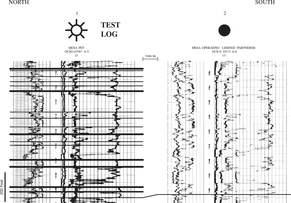
Figure 4-30 Two full-width electric logs, displayed side by side, with a series of arbitrarily named markers placed on the “type log.” Both logs are digital raster well log images with depth intelligence added to the depth track. (Published by permission of W. C. Ross and A2D Technologies.)
Configuring the width of each well log window to approximately two inches (for a 1 in. = 100 ft log scale) simulates overlaying two paper well logs for correlation by placing the two curves of greatest interest for correlation immediately adjacent to one another (Fig. 4-31a). The two-inch width of the log windows was chosen in order to display just one log curve from the full-width log. Choosing which well log curve is displayed in the two-inch wide log window (e.g., SP, GR, resistivity, conductivity) depends on which log curve is most useful for correlation. In our example, we place the SP and GR curves in this window. By creating narrow windows with single log curves (or single log tracks), a computer-screen display can simulate paper well-log overlay techniques and effectively increase the number of well logs that can be displayed on the screen at one time.
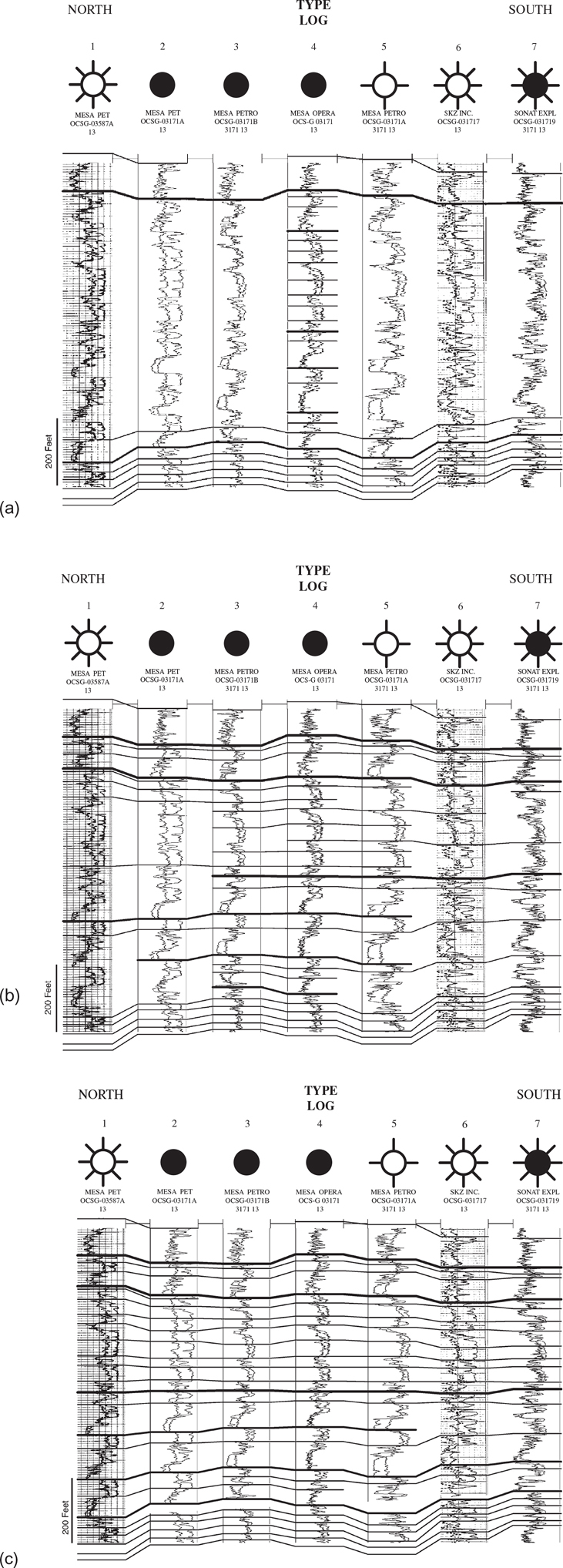
Figure 4-31 (a) Cross-section window configured to simulate paper-based log correlation. Closely spaced log windows, which here contain spontaneous potential and gamma ray curves centered within them, simulate the log overlay techniques used in paper-based methods. The type log contains a series of arbitrarily named markers to be used as starting points in a log correlation exercise. The wells in the cross section have an average spacing of less than one-quarter mile and were constructed with a combination of raster and digital (Log ASCII Standard) well log data. (b) Partially correlated panel of well logs illustrating the progression of correlation work from the central type log. (c) Completed correlation panel of well logs. (Published by permission of W. C. Ross and A2D Technologies.)
Computer log correlation can now proceed by simply pointing and clicking on each well log with the correlation tool at the various points of log correlation. Log slipping (or vertical scrolling) can be performed to help line up each of the logs prior to correlation itself.
To simulate the log annotation techniques used in paper-based correlation, the following procedure can be used. First, nominate a type well for the starting point in your correlation exercise. Next, place on the type log a series of markers (Fig. 4-31a). They are designated by an arbitrary naming convention, such as GM1 (generic marker 1), GM2, GM3, and their purpose is analogous to manual annotations on paper well logs. As with paper-based annotation, the markers should be placed with as much frequency as is needed to capture all the log character deemed necessary for detailed correlation.
Once the markers are placed on the type well (the starting point), the geologist can begin transferring each marker from well log to well log across a panel of wells (Fig. 4-31b and c). The correlation work proceeds by correlating all the wells in the study area using this level of detail. When creating a correlation section such as shown in Figure 4-31, the type log may be placed at the beginning of the section and repeated at the end of the section, rather than in the middle of the section, as in Figure 4-31. This procedure automatically loop-ties the correlations.
Whereas the level of detail in computer correlation may not be any higher than the paper-based log annotation techniques, computer-based correlation of markers carries the advantage that each marker top is automatically placed into a digital database of tops for each well. Consequently, as you build arbitrary cross sections through your 3D database of well control, all the marker correlation work will carry forward onto these cross sections. The power of this technology for geometric cross-sectional analysis, fault picking, and unconformity recognition is considerable, as we illustrate in the next section.
Example of Unconformity Identification
To illustrate the power of computer-based correlation for unconformity identification, we use an example of a correlation exercise from the Lewis Shale Formation within the eastern Green River basin in southern Wyoming (Fig. 4-32). The Lewis Shale overlies the non-marine and shallow marine Almond Formation (Winn et al. 1985).

Figure 4-32 (a) West-east stratigraphic cross section, hung on the B1 datum, constructed with conductivity curves centered within narrow well log windows. The light gray shading depicts sands within the Almond Formation. The darker gray pattern represents sands and shales of the non-marine Almond Formation, and the white region depicts shale facies within the Lewis Shale Formation. This cross section was constructed with well log images. Style of drawing correlations is from log edge to log edge. The cross section is eighteen miles in length with an average well spacing of less than two miles. The vertical exaggeration is 166:1. (b) Same cross section with correlation draw style changed to center-to-center of logs, which accentuates basin-fill geometries. Downlap on surface B1 is suggested. (c) Same cross section hung on the B2 stratigraphic datum. The higher datum changes the geometry of the unconformable relationship and suggests onlap versus downlap. (Published by permission of W. C. Ross and A2D Technologies.)
A subtle unconformity was discovered by careful well log correlation within the transgressive Lewis Shale, just above the Almond Formation. To illustrate how this unconformity was detected, we begin with a 10-well, west-to-east cross section constructed parallel to depositional dip across the Almond and Lewis Formations (Fig. 4-32a). The shallow-marine Almond Sandstone and the marine Lewis Shale represent the transgression of the Lewis seaway from east to west (right to left) on the section.
The on-screen correlation involved the use of arbitrarily named markers to perform high-resolution, time-stratigraphic correlations, following the sequence stratigraphic methodology of Van Wagoner et al. (1990). Following this strategy, we established a type well at the Davis Oil Armor State #1 (fifth well in cross section) and began correlating the initial markers across the panel of well logs. In the early stages of log correlation, it became apparent that there were distinct packages of rock within the Lewis Shale that could easily be distinguished and shown to be discordant with respect to one another along an unconformity surface (Fig. 4-32a). The discordant surface coincides with the top of a regional bentonite marker denoted as B1. The geometric discordance is enhanced through extreme vertical exaggeration (V.E. = 166:1). The vertical exaggeration is facilitated on a 21-inch computer screen by using narrow log windows, close well spacing, and by changes in correlation draw style. Figure 4-32a and b illustrate the visual advantages gained by changing the log correlation draw style from a conventional style where correlations are drawn straight across the log (i.e., edge-to-edge) to a style where the correlations are connected from the center point of each log (i.e., center-to-center). The use of center-to-center correlation drawing style smooths the connections between correlation points and provides a clearer view of both discordant relationships and subtle basin-fill geometries. Upon initial inspection, the discordant relationship (correlation markers terminating in an easterly or basinward direction against a common surface) was interpreted as depositional downlap (Fig. 4-32b). Computer-based cross-sectional analysis allows the interpreter to quickly choose an alternative cross-section datum to evaluate alternative interpretations of unconformity type. For example, in Figure 4-32c a higher marker (B2) is utilized as the stratigraphic datum, providing a view that would suggest the unconformity is an onlap unconformity.
Example of Fault Identification
For our second example, we illustrate the power of computer software to identify faults and interactively interpret missing section. We start with another cross section from the South Pelto area in the offshore Gulf of Mexico (Fig. 4-33a). The 6-well cross section contains numerous marker horizons that can be identified and correlated throughout the area. As discussed earlier in the chapter, using numerous markers in log correlation enables the geologist to quickly identify missing section due to normal faulting or erosional truncation. In Figure 4-33b we have added a well (Mesa Well No. A-6) and, due to the established high-resolution correlation framework, we can immediately determine that correlation markers A, B, and C are obviously missing in the A-6 well due to faulting. To determine the actual amount of section missing (in feet) due to faulting, we can pick a fault location and use a program function to “split” or “gap” the well log. The gap in the well log represents the amount of section missing due to normal faulting. The size of the gap is interpreted by interactively “dragging” down, or opening up, the boundary of the gap (Fig. 4-33c). Using one or more of the cross-section wells for reference, the geologist can reconstruct the amount of missing section by pulling down, or opening, the gap until the correlations above and below the gap are approximately parallel (Fig. 4-33d). In this example, we have interpreted the missing section to be approximately 215 ft thick. This value is also the amount of vertical separation, which is discussed in Chapter 7.

Figure 4-33 Cross section illustrating the technique to determine missing section. (a) Cross section with numerous markers demonstrating a continuous, unfaulted stratigraphic section. Average well spacing is less than one-quarter mile. (b) Same cross section with an additional well (Well No. A-6) that has missing section. The detailed correlation work demonstrates that the A, B, and C correlations are cut out by a fault (i.e., where correlations converge). (c) Same cross section with fault picked and log partially pulled apart (gapped) for Well No. A-6. (d) Same cross section with missing section interval fully interpreted and missing tops (A, B, and C correlations) placed within it. (Published by permission of W. C. Ross and A2D Technologies.)
The log-splitting tool allows you to create correlation cross sections hung on stratigraphic markers, with missing section (due to faulting or erosional truncation) displayed as missing section gaps. Once the gaps are interpreted, you can pick tops within the missing section to allow the cross section to be hung on missing top markers (Fig. 4-33d). The hand-generated equivalent to this computer method is shown in Figure 4-20b, for which a paper log was cut and pulled apart by the amount of missing section.
The use of high-resolution marker correlations, narrow window correlation displays, and interactive fault picking/gapping tools allows geologists to correlate hundreds of well logs within a short period of time. Correlation exercises are significantly aided by this fault-gapping technology. By picking and gapping faults during a correlation exercise, significant amounts of distortion related to missing section can be eliminated (compare Fig. 4-33b and d).
There are many advantages of computer-based log correlation over paper-based techniques. Perhaps the most significant are the capabilities for instant access to log data from a computerized database, automatic rescaling of images and digital data, rapid redatuming capabilities, and the ability to track and display hundreds of correlations/markers within a computerized database. For many traditional geologists, the transition to the computer has been a painful process. However, many of the concerns have been overcome by adopting some of the techniques described in this section.
Many geologists had expressed concern about being unable to see enough of the well log on the computer screen at one time. This is a legitimate concern. However, technology has improved dramatically in recent years, providing both high-resolution computer monitors and image-enhancement technologies, which allow several thousands of feet of section to be viewed on the computer screen for reconnaissance log review. Ultimately, geologists have agreed that the advantages of migrating to the computer outweigh the disadvantages of learning a new set of skills. As with geophysicists, who made the transition to geophysical workstations in the mid-1980s, geologists have rapidly made the transition to geological workstations. The enormous increase in productivity for geologists is on par with their geophysicist colleagues.
Repeated Section
A repeated section in a well is defined as a part of the stratigraphic section that appears twice on a log as the result of a fault, consequently lengthening the log section. A repeated section is commonly thought of as a compressional tectonic phenomenon, occurring as the result of a reverse fault pushing the stratigraphic section in the hanging wall up and over the same section in the footwall. Figure 4-34 illustrates the geometry required to result in a repeated section due to a reverse fault. A repeated section can also occur with a normal fault. In this situation, a repeated section requires a specific geometry between a normal fault and a directionally drilled well, or a normal fault that cuts a structure dipping at a steeper angle than the fault.

Figure 4-34 The geometry required for a repeated section due to a reverse fault.
So far in this book, we have looked at vertical and directionally drilled wells penetrating a fault in what is called the normal sense; that is, from the hanging wall (downthrown) fault block to the footwall (upthrown) fault block (Fig. 4-35). Figure 4-36 is a cross section illustrating the geological and deviated well parameters required to cause a repeated section in a log for a situation involving a normal fault. Geometries, as shown in Figure 4-36, are not uncommon in areas of directionally drilled wells. In offshore areas, deviated wells are drilled from a central platform location and are often designed to parallel a known fault (Fig. 4-37). In this way, a well may be drilled to penetrate a series of potential strata in the footwall (upthrown) block of an important trapping fault. If care is not taken to precisely map the fault and drill the well, it is possible for the well to cross the fault and enter the hanging wall (downthrown) block of the fault. In Figure 4-37, the well deviated toward the salt crosses a normal fault backwards, resulting in a repeated section. Also notice that by crossing the fault, the well does not penetrate productive Sand B, which is upthrown to the fault, but instead penetrates the nonproductive Sand B downthrown.
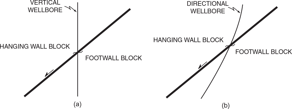
Figure 4-35 (a) A vertical well intersecting a fault in the normal sense (from hanging wall to footwall fault blocks). (b) A deviated well intersecting a fault in the normal sense (from hanging wall to footwall fault blocks).

Figure 4-36 The fault and deviated well parameters required for a repeated section resulting from a normal fault.
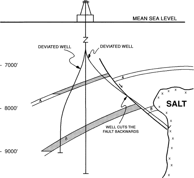
Figure 4-37 The well deviated toward the salt cuts the normal fault backwards (from the footwall block to the hanging wall block), resulting in a repeated section.
Figure 4-38 is an example of a repeated section resulting from an extensional (normal) fault. The amount of wellbore deviation is shown on the right of the log section. Notice that the deviation angle ranges from 40°45′ to 42°15′. The well was drilled to parallel a fault and to stay in the footwall fault block. Since wellbore deviation is measured from the vertical and fault dip from the horizontal, it is necessary to subtract the hole angle from 90 deg to compare its “dip,” or plunge, angle to that of the fault. By doing this, the well angle measured from the horizontal, for the section shown, ranges from 47°45′ min to 49°15′ min. Based on the fault surface map, the fault dip is approximately 52 deg. Therefore, the well inclines downward at an angle less than the fault dip, establishing a well/fault geometry similar to that shown in Figure 4-36. The result is the repeated section shown in Figure 4-38.

Figure 4-38 Repeated section in the Texaco LL&E Well No. 212 due to the well cutting a normal fault backwards. (Published by permission of Texaco, USA.)
Figure 4-39 is another excellent example of a repeated section resulting from a normal fault cut backwards by a deviated well. Observe that the footwall fault block is productive of hydrocarbons, whereas the hanging wall block is not.

Figure 4-39 Repeated section in a deviated well due to the well cutting a normal fault backwards. Notice that the footwall (upthrown) fault block contains hydrocarbons, while the hanging wall (downthrown) block is wet. (From Tearpock and Harris 1987. Published by permission of Tenneco Oil Company.)
The identification of a repeated section that has previously gone unrecognized can result in excellent prospect potential. Look at the generic situation shown in Figure 4-40. In this case, a well was designed to stay in the footwall of an important trapping fault. Good control on the fault was available at the time of drilling, but a fault surface map was not prepared. The well meandered across the fault, resulting in an unrecognized repeated section on the well log. The stratigraphic intervals penetrated in the footwall of the fault are productive of hydrocarbons, whereas the hanging wall interval from A to B are wet. The repeated section went unrecognized and, consequently, the wet intervals penetrated in the hanging wall were thought to be in the footwall and were condemned as nonproductive.
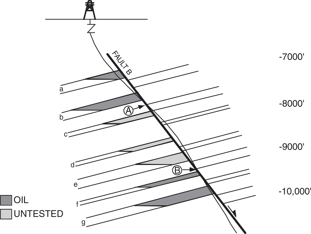
Figure 4-40 The identification of a previously unrecognized repeated section can result in a potential prospect. In this example, Sands c through e are untested upthrown to Fault B.
If an observant geoscientist recognizes the repeated section and understands that the nonproductive log section represents the well penetration in the hanging wall block, a new prospect can be generated in an area previously condemned. In Figure 4-40 the new prospect includes the stratigraphic sections c through e, present in the footwall block of the fault and not seen in the deviated well.
Estimating Restored Tops
A particular marker or stratum being mapped may be faulted out of one or more wells in the area of study. If this situation exists, it is often possible to estimate an upthrown (footwall) and downthrown (hanging wall) restored top for the missing marker or stratum in the faulted well(s). A restored top is defined as an estimated depth at a well for a specific marker or stratum that is faulted out of that well. Figure 4-41 illustrates the concept of restoring tops. An upthrown (footwall) restored top is the estimated depth of a marker or bed if the well were in the upthrown block and the marker not faulted out (i.e., if the fault were farther to the left in Fig. 4-41). Similarly, the downthrown (hanging wall) restored top is the estimated depth of the marker or bed if the well were in the downthrown block and the marker not faulted out (if the fault were farther to the right in Fig. 4-41). We strongly recommend that these data points be honored in structure mapping just as any other top obtained from well log data. This is important for maintaining the integrity of a structural interpretation and it provides additional information that aids in the actual structure contouring, as described in Chapter 8.
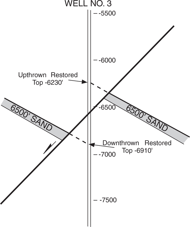
Figure 4-41 Basic concept of restoring tops. The upthrown restored top is the estimated depth in the well for the mapped horizon if the well were in the upthrown fault block. The downthrown restored top is the estimated depth in the well for the horizon if the well were in the downthrown block.
Vertical Wells
The procedure for determining the upthrown and downthrown restored tops (sometimes referred to as equivalent points) in vertical wells is discussed here and illustrated in Figure 4-42.
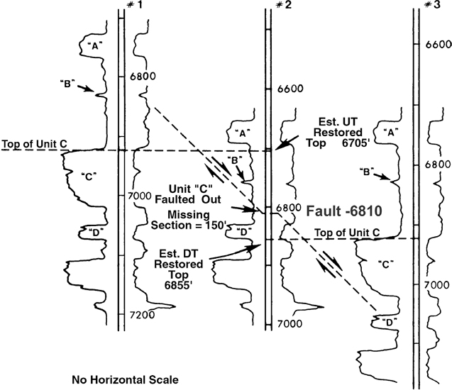
Figure 4-42 The method for estimating restored tops in vertical wells is shown by special correlation of the three vertical wells.
Figure 4-42 shows three vertical well logs positioned side by side with no horizontal scale. By correlation, we determine that there is a 150-ft fault in Well No. 2 and that the objective Unit C is faulted out. Well No. 1 is in the upthrown fault block and Well No. 3 is in the downthrown block. To determine the upthrown and downthrown restored tops, these two nearby wells are used.
Downthrown Restored Top for Unit C. To estimate the downthrown restored top, Well No. 3 in the downthrown fault block is used to correlate with Well No. 2. Identify a good marker, such as a field-wide sand or resistivity marker, in both logs above the faulted-out section. In Figure 4-42, the “B” marker is used as the marker in the wells. Line up the marker on both logs and correlate down the logs until the top of “C” is reached in Well No. 3. The equivalent measured depth reading for the top of “C” in Well No. 2 is 6855 ft. This represents the estimated depth for the top of “C” if the well were in the downthrown (hanging wall block).
Upthrown Restored Top for Unit C. To estimate the upthrown restored top, Well No. 1, which is in the upthrown block, is used to correlate with Well No. 2. Identify a good marker in both wells below the faulted-out section. In this case it is the “D” marker. Line up the “D” marker on both logs and correlate up the logs until the top of “C” is reached in Well No. 1. This equivalent depth reading for the top of “C” in Well No. 2 is 6705 ft. This represents the estimated depth for the top of “C” if the well were in the upthrown block.
The accuracy of the restored top estimates can be checked by subtracting the upthrown restored top from the downthrown restored top and then comparing the difference to the estimated value of the missing section for the fault. In this case, 6855 ft − 6705 ft = 150 ft. The difference in the restored tops and the amount of missing section in Well No. 2 are exactly the same. Therefore, we conclude that the estimated depths for the restored tops are reasonable.
A similar method to restore a top is to calculate the vertical distance that the top should be above or below the fault in the well. In the example shown in Figure 4-42, a point in upthrown Well No. 1 can be picked that is correlative to the fault pick in Well No. 2; it would be just above “D.” The true vertical thickness between that point and the top of Unit C can be determined. That thickness of 105 ft is equal to the vertical distance between the fault and the upthrown restored top of “C” in Well No. 2. In fact, that TVT can be used to calculate the restored top 105 ft above the fault, at 6705 ft, in Well No. 2. Similarly, the depth of the downthrown restored top in Well No. 2 can be determined by using the 45-ft TVT of the interval between the fault-correlative point and the top of Unit C in downthrown Well No. 3. In the next section, we use the TVTs of such reference intervals to restore the top of a unit faulted out of a deviated well.
In the example illustrated in Figure 4-42, the section in the three wells is approximately equal in thickness. What if a reference well is of different thickness than the well with a fault? That could result in an incorrect restoration of a top, so an adjustment to the thickness measured in the reference well is necessary. Simply apply a thickness ratio. Determine an average thickness ratio between the wells for stratigraphic intervals immediately above and below the fault in the faulted well. Then use that ratio to modify the TVT of each reference interval as measured in the reference well. For example, if the stratigraphic section in the faulted well is 0.80 as thick as that in the reference well, then multiply each reference interval measured in the reference well by 0.80 to provide a more accurate estimate for restoring each top.
The two restored tops should be honored in structure contouring of any mapped surface, whether it is a marker, sand top, particular stratum, and so on. If the map is referenced to sea level, measured log depths must be converted to subsea depths for structure mapping. The specific technique to apply the restored tops in structure mapping is discussed in Chapter 8.
Deviated Wells
All the wells are vertical in the example shown in Figure 4-42. Where deviated wells are present, the estimation of restored tops requires additional steps because TVTs must be used instead of the MLT in the deviated wells.
There are three separate cases for log correlation involving deviated wells: (1) a fault in a deviated well correlated with a vertical well; (2) a fault in a vertical well correlated with a deviated well; and (3) a fault in a deviated well correlated with another deviated well. Previously, we showed that missing section is defined in terms of TVT, and we also used TVT in restoring tops in vertical wells. When estimating restored tops in deviated wells, TVT must be used. Probably the most accurate way to estimate restored tops in deviated wells is to convert the deviated logs to TVT logs. In order to make a TVT log, bed dip and azimuth data are required in addition to the well deviation angle and well azimuth. If time, costs, or other factors prohibit the preparation of TVT logs, the restored tops can still be estimated with reasonable accuracy using the deviated well logs and applying a correction factor to derive TVTs. The correction of MLT to TVT was described in the section Estimating the Missing Section for Normal Faults.
For case No. 1, in which a fault in a deviated well is correlated with a vertical well, the same basic procedure for estimating a restored top using two vertical wells can be applied, with one significant variation. The depth of a restored top for the faulted-out unit cannot be transferred (projected) directly to the deviated well log from the top of the unit in the vertical well log, as it was in Figure 4-42, because the deviated well log depths are not vertical depths and the thickness of a given interval is not a TVT. A calculation for depth of each restored top must be made, and it is based on the TVT of a reference interval in the vertical well.
The procedure for restoring a top faulted out of a deviated well is shown in Figure 4-43. A fault is identified in the deviated Well No. 3 at a depth of −6810 ft, with a missing section of 100 ft (Fig. 4-43a). The B Sand is faulted out of the well. We wish to restore the upthrown and downthrown tops for the B Sand. Well No. 1 in the downthrown block and Well No. 2 in the upthrown block are available to estimate the restored tops.
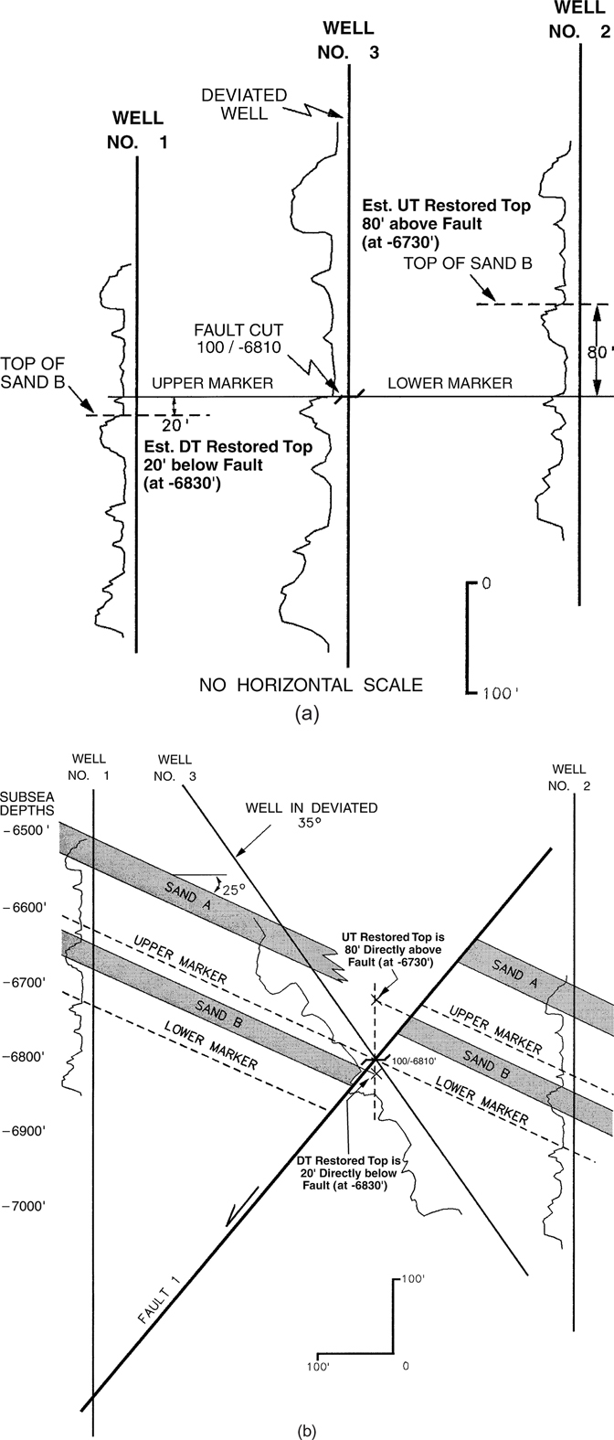
Figure 4-43 (a) The two vertical wells (Nos. 1 and 2) and the deviated well (No. 3) illustrate case No. 1, estimating restored tops for a unit faulted out of a deviated well. (b) A structural cross section containing the three wells shown in (a); it illustrates the precise positions of the restored tops with respect to Well No. 3: directly above (upthrown restored top) and directly below (downthrown restored top) the actual fault pick in the well. The top of Sand B in each fault block is projected to the appropriate restored top to establish the structural dip shown in the cross section.
Upthrown Restored Top for the B Sand. To estimate the upthrown restored top, identify a marker below the B Sand in Well No. 2 that is also in the faulted well. For this example, the lower marker used and shown in Well No. 2 is exactly at the fault in Well No. 3. By correlating up the logs, we determine that the top of the B Sand is 80 ft above the lower marker in Well No. 3. Since the marker is exactly at the fault in Well No. 3, the upthrown restored top for the B Sand in the well is 80 ft above the subsea depth of the fault. The subsea depth of the fault is −6810 ft; therefore, the upthrown restored top is −6730 ft. It is positioned vertically above the fault in the deviated well rather than within the inclined wellbore (Fig. 4-43b).
Downthrown Restored Top for the B Sand. The same procedure is followed to estimate the downthrown restored top. Using Well No. 1 in the downthrown fault block, identify a marker above but as close to the fault cut as possible. In this case, the upper marker used in Well No. 1 is exactly at the fault in Well No. 3. Correlate down the two logs from the upper marker until the top of the B Sand is reached in Well No. 1. Using the TVT of that interval, the restored top is calculated to be 20 ft vertically beneath the fault in Well No. 3, at −6830 ft (Fig. 4-43b).
The depths for the restored tops were not projected directly from faulted Well No. 3, as was done in the vertical well example (Fig. 4-42). Instead, for the upthrown restored top, the vertical distance from the fault-correlative point to the top of the sand in unfaulted Well No. 2 was subtracted from the subsea depth of the fault to estimate the upthrown restored top. Similarly, the vertical distance from the fault-correlative point to the top of the sand in unfaulted Well No. 1 was added to the subsea depth of the fault to estimate the downthrown restored top.
Observe that the correlation marker used to determine each restored top was chosen as the closest marker to the fault. It is recommended that, whenever possible, you choose a correlation marker as close to the fault as possible in order to minimize any errors due to correlation or due to stratigraphic variations between the wells being used.
In Figure 4-43b, which is a structural cross section through the three wells, an X is placed 80 ft vertically above and 20 ft vertically below the fault in Well No. 3. These X’s show the precise position of the upthrown and downthrown restored tops for the B Sand. It is important to understand that the restored tops are located vertically above and below the location of the fault in the well and not within the deviated well either in cross-section view or in map view. This understanding is critical when using these restored tops in structure mapping.
The fact that restored tops in a deviated well are plotted directly above the location of the fault in the well can cause complications when using a workstation. We are not aware of any interpretation software that will plot a restored top directly above the fault cut. If the restored top is stored with other tops from the well in the software database, the restored tops will plot along the wellbore, not directly above the fault cut. This will cause the restored tops to be plotted in the wrong spot on a map. It is possible that an upthrown restored top may be plotted in the downthrown fault block and vice versa. One possible solution is to store the restored tops in a pseudo-well as digital control points at the same X-Y position as the fault cut. The challenge of using restored tops in structure mapping using a workstation is discussed in more detail in Chapter 8.
The 100-ft difference between the downthrown and upthrown restored tops agrees with the 100 ft estimated for the missing section in the well. Therefore, we conclude that the depths for the estimated restored tops are reasonable. The depth difference between the downthrown and upthrown restored tops should always agree with the amount of missing section estimated for the fault.
For cases 2 and 3, in which a fault in a vertical well is correlated with a deviated well or a fault in a deviated well is correlated with another deviated well, the procedure is basically the same as for case 1 with one exception. When an unfaulted deviated well is used as a reference, the TVT from a marker to the mapped (faulted) horizon must be calculated to accurately estimate the restored tops. The measured (deviated) log thickness cannot be used to properly estimate restored tops. For example, if Well No. 2 in Figure 4-43a were a deviated well, the interval thickness of 80 ft measured from the upper marker to the top of Sand B would have to be corrected to TVT before calculating the subsea depth of the upthrown restored top.
Unconformities
Unconformities are present in all geological settings, especially on steeply dipping growth structures. Excellent hydrocarbon traps can occur at unconformities where overlying impermeable rocks form seals for reservoirs. Therefore, it is important to recognize, analyze, and often map unconformities in the subsurface.
There are a host of interrelated versions of the broad term unconformity. Some are primarily erosional, some are nondepositional, and others are combinations of both. The subject of unconformities is extensive and beyond the scope of this book. We present important information on the recognition of unconformities during electric log correlation.
An unconformity appears on an electric log as missing section. Since missing section can be due to an unconformity or to a normal fault, care must be taken during correlation so that an unconformity is not mistaken as a fault. In this section we discuss several general guidelines to follow during correlation to recognize an unconformity.
Structural dip commonly is different above and below an unconformity. Dipmeter data can be used to indicate this change in dip. The structural dip below an unconformity is usually steeper (Fig. 4-44).

Figure 4-44 (a) Well log correlation can be used to recognize an angular unconformity. (b) If an onlap sedimentary sequence is deposited above an angular unconformity, certain log correlation guidelines can be used to recognize the unconformity.
If missing section is recognized in two or more wells at the same or nearly the same correlative horizon, such as “C” in Figure 4-44a, an unconformity, rather than a fault, should be suspected.
The amount of missing section resulting from an unconformity increases in the up-structure direction. This is illustrated in Figure 4-44. The missing section in Wells No. 1, 2, and 3 increases in the up-structure direction; Well No. 3 has the least amount of section missing and Well No. 1 has the greatest amount missing.
The stratigraphic section below an unconformity is truncated in a younger sequence in down-structure wells than in up-structure wells. The truncated sequence becomes older in the up-structure direction. In Figure 4-44a, the sedimentary sequence just below the unconformity in Well No. 3 (the G interval) is younger than the K interval in Well No. 1. To recognize the sequence trend, you must correlate up the well logs.
If the depositional environment results in an onlap sedimentary sequence (Fig. 4-44b) rather than the sequence shown in Figure 4-44a, the missing section in logs correlated in the up-structure position increases above and below the unconformity. The sedimentary sequence just above the unconformity is younger in the up-structure direction.
Unconformities must be mapped. Since an excellent hydrocarbon trap can occur at an unconformity, a map of the unconformity is vital. In order to identify the intersection of the unconformity and the underlying sedimentary sequence, an unconformity map must be integrated with structure maps of relevant surfaces within that sequence. The mapping techniques required are discussed in Chapter 8.
Figure 4-45 illustrates the use of a dipmeter to aid in the identification of an angular unconformity. The figure also shows a dipmeter response to beds affected by the proximity of salt with an overhang. The dipmeter reaches a maximum dip of 62 deg at about −6500 ft; thereafter, the dip slightly flattens to 40 deg at TD. This change in dip is in response to the proximity to the salt face. Such dipmeter responses can be used in evaluating a salt feature for possible overhang, with potential stratigraphic section beneath it.
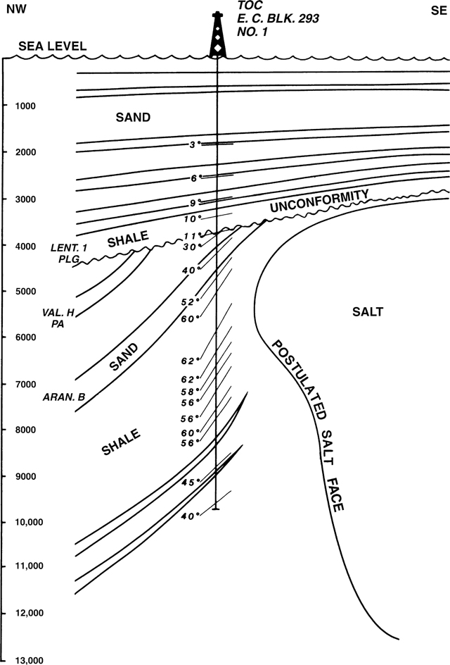
Figure 4-45 Dipmeter data can be used to recognize an unconformity in the subsurface. (Published by permission of Tenneco Oil Company.)
In the mid-1990s, Dr. Richard Bischke developed a powerful new technique for evaluating structural and stratigraphic information from well log as well as seismic data. This technique, today known as the Multiple Bischke Plot Analysis (MBPA), has numerous applications (Bischke 1994b; Bischke et al. 1999). One application of the technique is to assist in the differentiation of unconformities from faults in well logs where missing section is present. It is a rapid, robust, and powerful method for application with unconformities, as well as validation of general log correlations (see Chapter 13).
Annotation and Documentation
The importance of good, accurate documentation cannot be overemphasized. The generation of good quality maps depends on a volume of accurate data. These data include faults, horizons, tops and bases of stratigraphic units, net sand, net pay, and so on. In this section, we illustrate a recommended method of annotating 1-in. and 5-in. electric logs and documenting the log data.
In Figure 4-2 we illustrated the importance of marking logs with recognizable symbols and the use of color. These markings are a form of annotation. They identify your correlations. The logs in Figure 4-2 are of intervals that do not contain any hydrocarbons. There are some additional data that should be annotated on a 1-in. or 5-in. log with recognized pay. Figure 4-46 illustrates the additional data that should be annotated in the pay section on a 1-in. log. The annotation includes the name of each pay zone, perforation intervals, well status, cumulative production from each interval produced and a note on why each interval went off production, and the measured and subsea depth for the top of each important productive interval. Any intervals that appear productive on the log but have not been produced should be noted, such as Sands 2 and 6A in Figure 4-46. If sidewall cores are taken, the results of analyzing these cores should be posted. Finally, any recognized faults must be indicated on the log, such as Fault F, which faults out Sand 3 at a log depth of 8350 ft. It is important to note that the fault cut in Figure 4-46 includes the amount of missing section and the well or wells from which the missing section was determined.
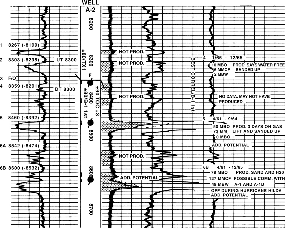
Figure 4-46 Electric log annotation in a hydrocarbon-bearing (pay) section. (From Tearpock and Harris 1987. Published by permission of Tenneco Oil Company.)
Annotating data when correlating logs on a workstation is, in many cases, easier as the software automatically enters tops into a database. Some data, such as missing section associated with a fault, is usually not included in the database automatically. Most software interpretation packages include places where additional notes, such as missing section, can be added to the database. It is important that interpreters use these features and record all important data. If picking up an interpretation project from a colleague, it is also important to check the note section of a database. Unlike a note handwritten on a paper log, you will never see a note in a computer database unless you look for it.
The annotation of a detailed 5-in. log is crucial, and an example is shown in Figure 4-47. The information annotated includes the name of productive zone, measured and subsea depth of the correlated tops, perforation intervals and corresponding production, well status, net pay counts, limit of pay (full to base of interval or water contact), and basic core data (at least the porosity and permeability data). Notice that the net pay on the 5-in. log in Figure 4-47 is assigned per 10-ft intervals on the left side of the log. This annotation is used to support the net pay count and later in preparation of net pay isochore maps.
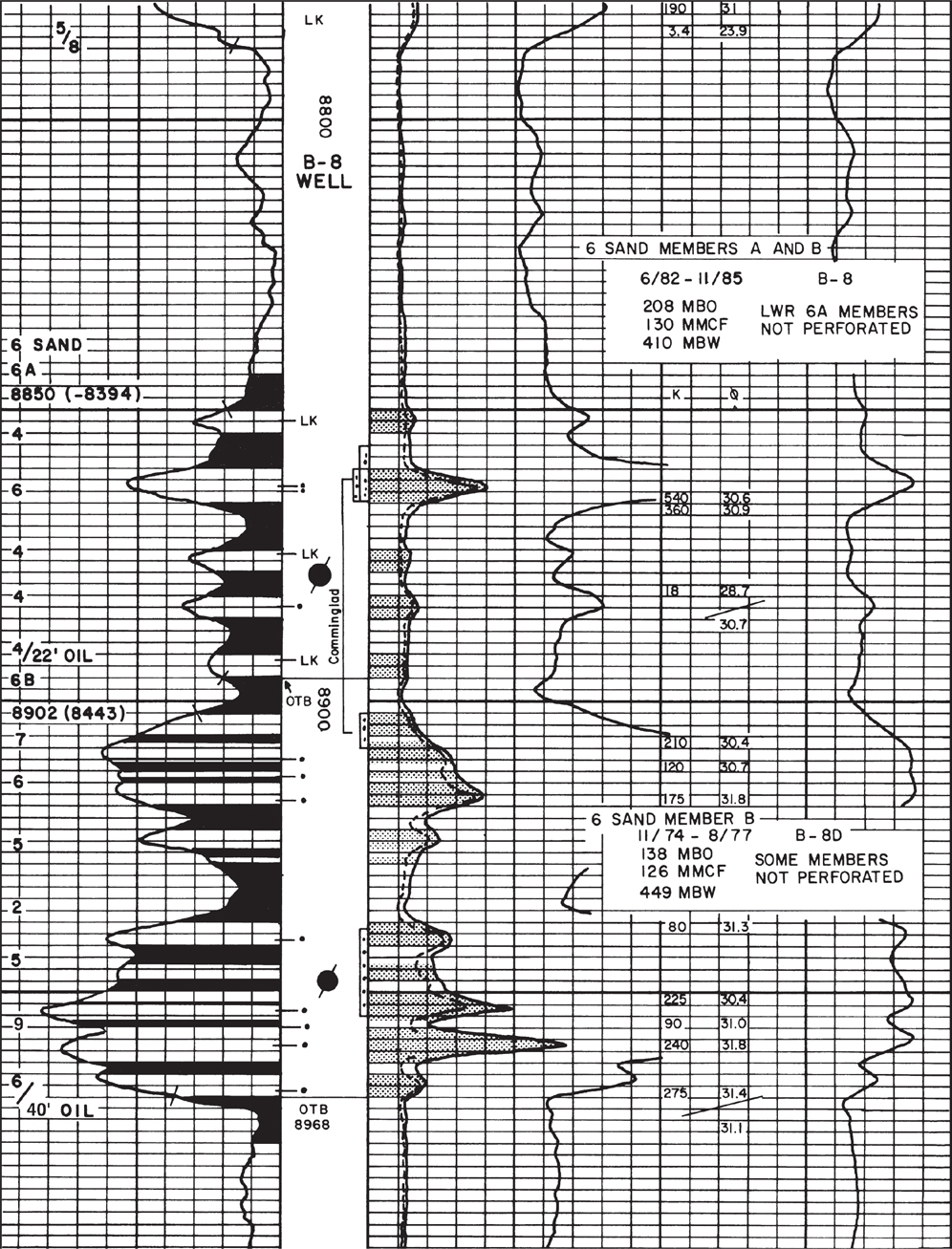
Figure 4-47 Annotation of a detailed 5-in. log. (Modified from Tearpock and Harris 1987. Published by permission of Tenneco Oil Company.)
Finally, the documentation of well data means recording it in some format that can be easily used. There are various types of manual and computer data sheets available for documenting mapping parameters. These data sheets should be used at all times to document the log correlation data.