Chapter 6. Cross Sections*
* For all figures in this chapter (in the printed book only), see the preface for information about registering your copy on the InformIT site for access to the electronic versions in color.
Introduction
A contour map depicts the horizontal plan view configuration of a single attribute of a stratigraphic unit, such as structure, thickness, and percent porosity. In contrast, a cross section depicts the configuration of many units as typically viewed in a vertical plane. Since a map or cross section alone cannot represent the complete subsurface geological picture, both must be used to conduct a complete and detailed study.
Geological cross sections constitute a very important geological exploration and exploitation tool. They are useful in all phases of subsurface geology as well as in reservoir engineering. Cross sections are used for solving structural and stratigraphic problems in addition to being employed as finished illustrations for display or presentation. Used in conjunction with maps, they provide another viewing dimension that is helpful in visualizing a geological picture in three dimensions.
If a cross section is oriented perpendicular to the strike of the structure, it is termed a dip section. If the section is oriented parallel to the strike of the structure, it is called a strike section. Finally, if the orientation is oblique to the structural axis, it is termed an oblique section.
Various data can be used to construct a vertical cross section. It can be based on surface data (dips), electric well log data (markers, unit tops and bases, dips, and faults), seismic data, or entirely from completed subsurface maps. As mentioned in Chapter 1, all available data should be used in the preparation of a subsurface interpretation, whether it is in the form of a structure map or cross section.
Planning a Cross Section
Prior to making a cross section, ask yourself a number of questions regarding the planned section construction. The answers to these questions facilitate the preparation of the section and improve its value as an aid to solving problems or illustrating the final geological picture.
What is the purpose of the cross section? Is the section going to be used as a structural or stratigraphic aid to solving problems? Is it going to be used as a communication device to illustrate the final geological picture? Will the section show the gross geological framework or be designed to show significant detail? What sources of data are to be used in the construction? Should the section be prepared true to scale (with the same vertical and horizontal scales) or at an exaggerated scale? What datum is to be used? The answers to these questions provide insight into the planning and preparation of any proposed cross section.
Initially, you must determine the specific objective for preparing a cross section. If it is to be prepared to aid in the interpretation of the structural framework and solve problems related to faulting and structural dip, then the section required is a structural cross section. If the intent of the section is to solve stratigraphic problems relating to detailed correlations, permeability barriers, unconformities, facies changes, or changes in depositional environments, then a stratigraphic cross section is needed. A structural or stratigraphic section can be used as a visual aid to communicate or illustrate, as well as to solve, problems. The intent will affect the preparation of the section.
The next step in preparing a cross section is to choose the orientation of the line of section. The choice is dependent first on the type of section you intend to prepare (structure or stratigraphic); second, on the type of geological structure (i.e., diapiric, extensional, compressional, or strike-slip); and third, on the data to be used in the section (well logs, seismic data, structure maps, or surface data).
Finally, the scales of the proposed section must be selected. Two separate scales must be considered: the vertical and the horizontal. The scales used are dependent on the type of section being prepared, the actual length of the section, data used, and desired detail. Whenever practical, use the same horizontal and vertical scales. However, there may be a special consideration that requires the section to have different vertical and horizontal scales. Often, the vertical scale is larger than the horizontal, and where this situation occurs, the section is said to have vertical exaggeration. Each of the specific conditions that go into the planning and preparation of a line of section are discussed in detail in this chapter.
Structural Cross Sections
Structural cross sections illustrate structural features such as dips, faults, and folds (Silver 1982). They are usually prepared to study structural problems related to subsurface units, fault geometry, and general correlations. Such problem-solving is accomplished by enabling you to visualize the subsurface structure in a vertical plane. Electric well logs (Fig. 6-1) or well log sticks (Fig. 6-2) can be used in the construction of structural cross sections. There are times when electric logs are not available and other data must be used. These data could include drill-time logs, core data, and lithologic logs prepared from cuttings descriptions.

Figure 6-1 Structural cross section prepared from electric log data. (Modified from Oil and Gas Fields of Southeast Louisiana, v. 3, 1983. Published by permission of the New Orleans Geological Society.)
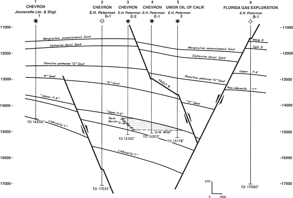
Figure 6-2 Structural cross section prepared using well log sticks. (Modified from Oil and Gas Fields of Southeast Louisiana, v. 3, 1983. Published by permission of the New Orleans Geological Society.)
Structural cross sections are drawn in the direction of interest. The section can be oriented perpendicular, parallel, or oblique to structural strike. For solving structural problems, it is common for the line of section to be laid out in the dip direction or over the crest of a structure. A line of section parallel to the dip of a fault is best for solving fault problems. In a complex area such as that of a faulted diapiric salt structure (Fig. 6-3), the evaluation of the structure, salt, and fault geometry may require a number of cross sections to be laid out in the direction of structural dip and perpendicular to fault strike. Each structure and the problems to be solved must be evaluated individually as to the planned direction and the number of sections required to adequately study the geological feature.
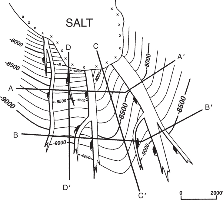
Figure 6-3 Typical cross section layout for a complex piercement salt structure.
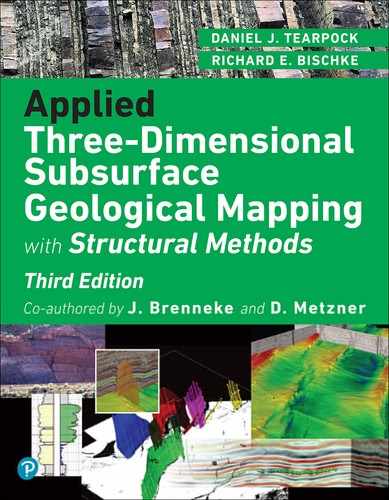
Oil and gas wells do not normally lie in a straight line, as shown in Figure 6-4a, and so the direction of a planned cross section may not be in a straight line. Instead, line segments between adjacent wells may vary in length and direction, giving the line of section a zigzag appearance (Fig. 6-4b). With a zigzag section, wherever the direction of the line of section changes, the apparent dip of horizons and faults on the section also changes. An example of such a change can be seen in Figure 6-1 for Fault B. Notice that the dip of the fault changes from 46 deg between Wells No. 3 and 4 to about 18 deg between Wells No. 4 and 5. This change indicates that the line of section between Wells No. 3 and 4 is perpendicular or nearly perpendicular to the strike of Fault B; but between Wells No. 4 and 5, the line of section is more parallel to the strike of the fault. These apparent changes in fault dip are illusions of subsurface geometry caused by the orientation of the line of section. Such illusions must be considered when laying out any line of section in order to prevent confusion to an observer and also to make sure that the section shows what it was intended to show.
Figure 6-4 (a) A cross section oriented through wells that form a straight line. (b) A zigzag line of section formed by line segments between adjacent wells.
We recommend that structural cross sections be drawn with the same horizontal and vertical scales whenever possible. With the same scales, the cross section is prepared true to scale with no vertical or horizontal exaggeration. At times, however, exaggeration is required to permit legible vertical detail. The effects of vertical exaggeration are discussed in detail later in this chapter.
Electric Log Sections
When preparing cross sections with electric logs, certain procedures are helpful in maximizing the usefulness of the section. These procedures will vary depending on whether you are making a cross section using paper logs or making a cross section on a workstation. We discuss using paper logs first.
The logs that are chosen for a section must fit the scale of the cross section. The logs may need to be enlarged or reduced to make the scale equal to that of the cross section.
If possible, use the same vertical and horizontal scale. This is usually convenient for field studies; however, regional or semiregional sections may require exaggerated vertical scales to get them down to a manageable size.
Data must be legible. Log heading data, correlations, depths, and so on, may have to be posted after the section is laid out in order for them to be legible.
How are electric logs mounted on a manually generated cross section? The procedure usually begins with the preparation of a film positive for each of the original logs to be used in the section. If required, the logs are reduced to the appropriate vertical scale to accommodate the section. The film positives are normally taped on coordinate grid cross-section paper with the correct proportional horizontal spacing between wells. It is good practice to plot your line of section on a well basemap or structure map (Fig. 6-13) so the spacing between well logs for the section can be measured directly from the basemap. For a structural section, the logs are normally hung with sea level as the reference datum. Therefore, the measured log depths must be converted to subsea depths for vertical position on the section. Finally, an ozalid or xerographic print of the cross-section base is made, and you are now ready to begin the cross-section interpretation.
Cross sections are more easily prepared if you use a computer. In a few simple steps, a line of section is laid out with proportionally spaced wells that can be hung on a given datum. The datum is readily changed and the logs are easily manipulated in making interpretations. The procedures are described in the section Cross-Section Construction Using a Computer.
As the first step in an interpretation, we recommend that all recognized correlation markers, as well as locations of faults in each well, be indicated on the logs used in the section. The faults can be connected from well to well to reflect the proposed fault interpretation. Lastly, in developing your interpretation, lines can be drawn from well to well connecting the correlation markers, with the lines being offset across faults (Fig. 6-5). Straight-line sections are typically used to initially evaluate a structure (Fig. 6-8a). They portray the dip in straight-line segments, so such features as variations in dip between wells will not be apparent. Although such a section does not represent the true attitude of the structure, during the initial phases of a study it provides significant information on the general structure, fault geometry, and correlations.
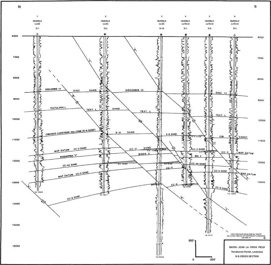
Figure 6-5 Completed structural cross section from Bayou Jean La Croix Field, Terrebonne Parish, Louisiana. (Reprinted from Oil and Gas Fields of Southeast Louisiana, v. 3, 1983. Published by permission of the New Orleans Geological Society.)
Cross sections usually go through several stages of revisions, with each such revision improving the accuracy and reasonableness of the interpretation. Remember that the final cross-sectional interpretation must agree with the completed geological maps, be geologically reasonable, have 3D geometric validity, and conform to the structural style of the area. If possible, cross sections should be retrodeformable or structurally balanced (see Chapter 9).
Figure 6-5 is a completed structural cross section from the Bayou Jean La Croix Field in Terrebonne Parish, Louisiana. It is a good example of what is called a finished illustration (Langstaff and Morrill 1981) structural cross section prepared from electric well logs (1 in. = 100 ft) and finished structure maps on the various horizons shown. The section is geologically reasonable for the tectonic setting, illustrating the subsurface structural geology, including fault geometry, correlations, and areas of hydrocarbon accumulation. The section was prepared true to scale with the same horizontal and vertical scales shown graphically in the lower right-hand corner of the section.
Stick Sections
An alternative to electric logs is the use of log sticks in the preparation of a cross section. A stick is defined as a vertical or deviated line that represents an electric log. A stick section has several advantages over the electric log section, including simplicity, clarity, and ease of construction (Lock 1989).
Since sticks do not show any correlation data (stratigraphic correlations or faults), it is necessary to record the depth of all pertinent correlations and faults obtained from the actual electric logs. Stick sections are often used to solve structural problems because of their simplicity and lack of clutter. A typical stick structure cross section is shown in Figure 6-2. This is the same cross section shown in Figure 6-1, which incorporates the actual electric well logs.
Stratigraphic Cross Sections
Problems related to changing stratigraphy require a stratigraphic cross section. They are drawn to illustrate stratigraphic correlations, unconformities, permeability barriers, stratigraphic thickness changes, facies changes, and other stratigraphic characteristics. Many of the comments made about structural sections also apply to stratigraphic sections. Vertical and horizontal scales must be assigned, the line of section laid out based on the intent of the section, a datum chosen, and the logs prepared to place on the cross section. The datum for a stratigraphic cross section is normally chosen as some stratigraphic marker with the section set up so that the chosen datum is horizontal. By using a horizontal datum, the distorting effects of structure (folds and faults) are eliminated. This is equivalent to unfolding and unfaulting the strata. Figure 6-6 is an example of two stratigraphic cross sections from southwest Kansas/northwest Oklahoma, each hung on a specific stratigraphic datum. These sections were prepared as part of a detailed study to evaluate the complexities of the structural and stratigraphic factors controlling the trapping of hydrocarbons in the Morrowan Sandstones (Mannhard and Busch 1974).
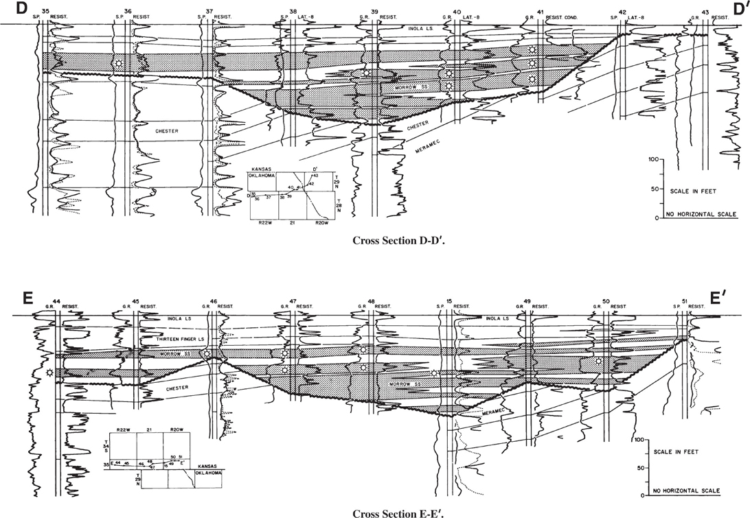
Figure 6-6 Two stratigraphic correlation sections prepared to evaluate stratigraphic complexities in the Morrowan Sandstones. (From Mannhard and Busch 1974; AAPG©1974, reprinted by permission of the American Association of Petroleum Geologists (AAPG) whose permission is required for further use.)
In preparing structural cross sections, recall that you had the choice of using the actual electric well logs or stick representations of the logs. For stratigraphic cross sections, the actual well logs are usually used, since the work involves solving problems related to the lithology. Changes in lithology from well to well can be evaluated only with real log data, although in special cases stick sections may be appropriate.
In the preparation of a stratigraphic section, the choice of an appropriate marker bed to use as the datum is extremely important. The choice of a poor datum can pose problems, such as incorrectly illustrating the original configuration of the stratigraphic units under study. For example, a poorly chosen datum may incorrectly depict an actual channel sand as a bar.
Remember, one of the primary objectives in laying out a stratigraphic section is to reconstruct the sand geometry at the time of deposition or shortly thereafter. When working in areas of predominant sand/shale deposition, keep in mind that sands and shales compact to differing degrees. The effects of differential compaction as the result of sediment burial are recorded on the electric logs. If you have a good idea of the environment of deposition for the sands being evaluated, the choice of the datum may be relatively easy. If the environments are in question, however, you should ask yourself which marker is most likely to have been close to horizontal at the time of deposition.
Figure 6-7 illustrates three cross sections of the Pennsylvanian Anvil Rock Sandstone, with each section having a different reference datum. In the upper section, the No. 7 coal seam above the sand is chosen as the datum. Figure 6-7 is one of those special cases where log sticks are appropriate for a stratigraphic section. With this reconstruction, the cross section does not show the effects of draping over the sand. In the middle section, the top of the Anvil Sandstone is used as the datum. By using this datum, the sand may give the appearance of a channel-fill sand regardless of the sand’s actual original configuration. The bottom section using the No. 5 coal seam below the sand is the best choice in this particular situation because this last section depicts the Anvil Sandstone as a channel-fill sand that shows the effects of differential compaction. The channel sand interpretation is also supported by the lateral truncation of the 5A and 6 coal seams against the sand. If the intent was to reflect the geometry at the time the channel was active and the Anvil Rock Sandstone was deposited, the middle section hung on the sandstone itself would come closest to showing this geometry. Figure 6-7 illustrates the fact that stratigraphic sections may be highly exaggerated to emphasize a specific point, as this figure has a vertical exaggeration of greater than 50:1.
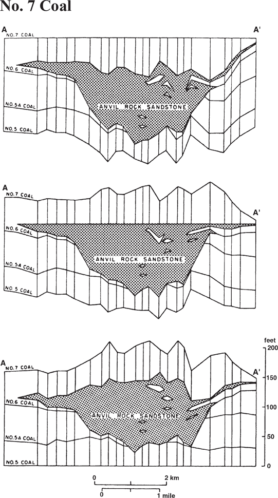
Figure 6-7 The choice of a reference datum is very important in the construction of a stratigraphic cross section. Three stratigraphic cross-sectional interpretations of the Anvil Rock Sandstone are shown based on three different reference data (Potter 1963).
We emphasize that care must always be taken when choosing the stratigraphic datum for a stratigraphic cross section. There are no actual rules of thumb to apply when choosing the datum. However, the answers to the initial questions that should be posed prior to constructing a section often can serve as a guide in your choice of the best datum.
Problem-Solving Cross Sections
Cross sections can be very useful in helping to solve structural and stratigraphic problems from the earliest through the later stages of a project. We call such sections problem-solving cross sections. As stated earlier, electric logs are usually required if the problem is stratigraphic. If the basic problem is structural, stick sections may be useful in solving fault and structural geometry problems.
Two different stick sections using the same data are shown in Figure 6-8. Figure 6-8a is an example of a problem-solving cross section utilizing the straight-line method of illustrating the geological interpretation. With this method, straight lines are drawn from well to well representing the horizon and fault correlations. Obviously, the straight lines between wells may not illustrate the true geological picture, such as changes in bed dip between control points. However, in the initial stage of a geological study, this type of section is very helpful in evaluating alternate correlations and fault and structural interpretations. Remember, the interpretation must be geologically reasonable and have 3D geometric validity.
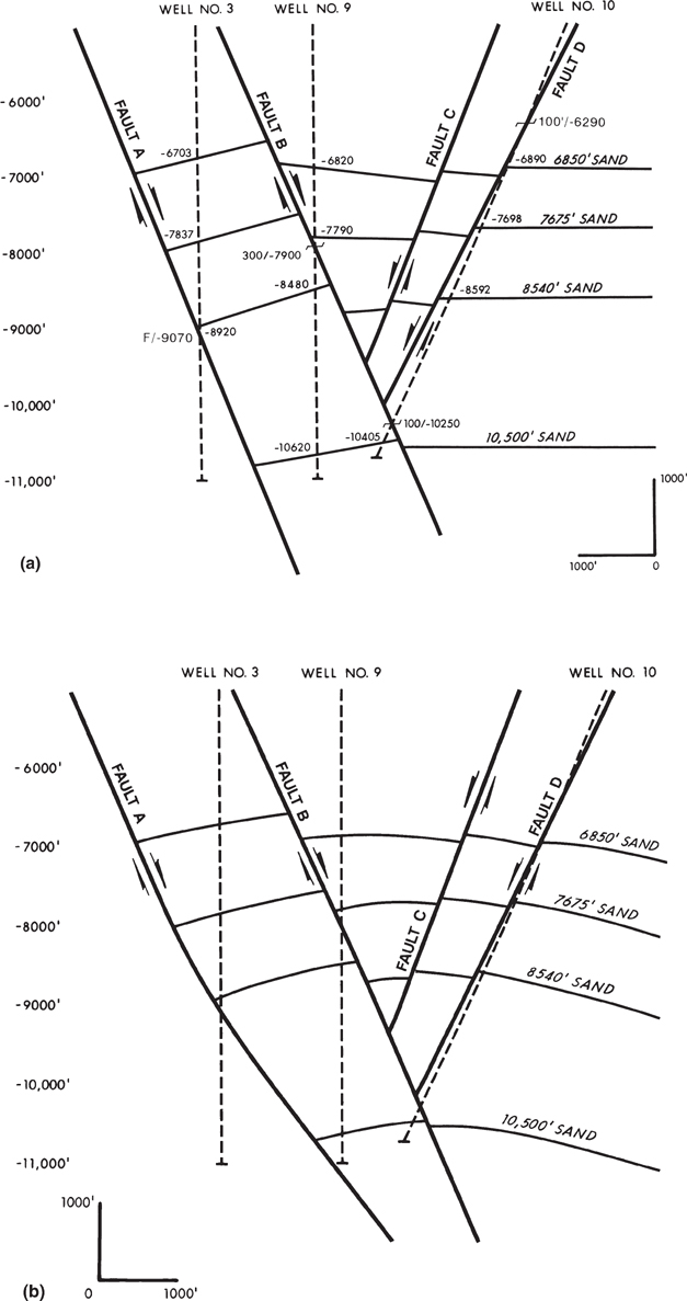
Figure 6-8 (a) Straight-line problem-solving cross section. (b) Finished illustration cross section constructed from completed fault and structure maps (compare this with Fig. 6-8a).
Finished Illustration (Show) Cross Sections
A finished illustration (show) cross section illustrates the final interpretation. It is constructed after all the fault and structure maps have been prepared, and it is used to complement the fault and structure maps. Finished illustration cross sections also serve as visual aids to communicate and present the final geological interpretation.
Figure 6-8b shows a completed finished illustration cross section for the initial interpretation shown in Figure 6-8a. Observe that the correlations between wells reflect the true geometry of the horizons and faults as opposed to the initial straight line interpretation.
Figure 6-9a and b present the details of constructing a finished illustration cross section from electric well log control and completed subsurface maps (in this case, a structure and fault map). The section is a dip section crossing a normally faulted anticlinal structure. The figures depict the data used in constructing the 6850-ft Sand and Faults A, B, C, and D on the finished illustration cross section. The final illustration cross section constructed from all the fault and structure maps is shown in Figure 6-8b.

Figure 6-9 (a, upper) Structure map on the top of the 6850-ft Sand. Line of cross section shown on map.(a, lower) Details for construction of a finished illustration section for the 6850-ft Sand. (b, upper) Fault surface map for Fault B. Line of section shown on map. (b, lower) Detailed construction for Fault B for incorporation into finished illustration cross section.
We can review Figure 6-9a and b to illustrate the actual procedure for constructing this type of cross section by hand. The upper part of Figure 6-9a is a structure contour map on the 6850-ft Sand. The line of section, drawn on the structure map, starts at the downthrown trace of Fault A, continues through Wells No. 3, 9, and 10, and terminates at the −7100-ft contour line upthrown to Fault D.
It is always a good idea to review the planning and preparation procedures presented earlier before beginning any cross section until you feel that you are thoroughly familiar with them. The first task for a manually drawn cross section is to prepare the cross-section coordinate grid paper, with the logs proportionately spaced, and then begin plotting all appropriate available data points. Since all the data are acquired from completed maps and accepted log correlations, it is not necessary to place the actual electric logs on the section; however, this is a matter of personal preference. The first points to plot are those for the top of the 6850-ft Sand, taken from the structure map in Figure 6-9a (upper). Starting with Well No. 3, the first data point to place on the section is the top of the sand in this well, which is at a depth of −6703 ft. This point, shown at Well No. 3 on the structure map, is plotted at the appropriate depth on the log stick for Well No. 3 on the cross section (position A). The second data point is the intersection of the section line and the −6700-ft structure contour line on the structure map, 100 ft southeast of Well No. 3. This −6700-ft subsea depth point is plotted on the cross section 100 ft from Well No. 3 (position B). The third data point is the intersection of the section line with the −6600-ft contour line on the structure map. This point is 725 ft southeast of Well No. 3 and is plotted on the cross section at position C.
What is the fourth data point? It is the intersection of the section line and the upthrown trace of Fault B, which is at an estimated subsea depth of −6585 ft and measures 900 ft from Well No. 3. This point is plotted on the cross section at position D.
This procedure is continued for each measurable data point along the line of section on the structure map. Although there are no wells north of Well No. 3, the section extends to Fault A using all contour lines as data points. It should be noted that measurable data points include such items as gas/oil contacts, oil/water contacts, and upthrown and downthrown fault traces. You will also notice that there is an obvious structural crest about 150 ft south of Well No. 9. The crestal position and its subsea depth have been estimated and incorporated into the cross section. Remember that this section is being constructed after the structure maps are in their final stages of completion, and all data shown on the maps should be used in the construction of the cross section.
Each point for this cross section is identified on the structure map along the section line and plotted on the cross section. When all the data points are plotted and connected with a correlation line, a detailed interpretation of the 6850-ft Sand is illustrated in cross-sectional view (lower part of Fig. 6-9a). This procedure should be completed for all the sands planned for the cross section.
Turning to Figure 6-9b upper, we see a contour map for Fault B with the line of section drawn on the map. Following the same procedure outlined for the 6850-ft Sand, the location of each fault data point is identified on the fault surface map and plotted on the cross section in the lower part of the figure. The same procedure is followed for Faults A, C, and D.
We now have completed the plotting of all the available data points for the 6850-ft Sand and all the faults for the finished illustration cross section in Figure 6-8b. The interpretations of the other sands were constructed using the same procedure just outlined. The result is a detailed cross section representing an accurate picture of the structural interpretation of the horizons and faults in a vertical plane.
In summary, a finished illustration cross section is important for several reasons. It serves as a visual aid for presenting a completed geological interpretation and can also be helpful in identifying mapping problems that might otherwise go undetected, particularly in fields with closely spaced productive sands. An accurately detailed cross section might indicate any number of mapping “busts,” such as areas where thickness compatibility between horizons has not been honored. The cross section in Figure 6-10, prepared to evaluate cross-fault drainage, is an example of a detailed finished illustration cross section constructed almost exclusively from final structure maps for each of the horizons shown on the section. The section shows that the interpretation for each horizon, the faults, and the intersection of the faults with the individual horizons is geologically reasonable for the most part. However, a few areas on the cross section appear to indicate some minor geological busts, which are highlighted by asterisks. Although none of these problems seem to be serious, the fact that they are visible shows the sensitivity of this detailed cross section to interpretation error.
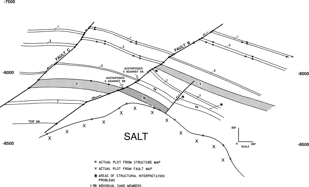
Figure 6-10 A detailed finished illustration cross section constructed almost exclusively from completed maps, including fault maps, structure maps on the top and base of each of the seven stratigraphic units shown, and a salt map. Notice that the detailed section indicates that the 6 Sand downthrown to Fault B is in juxtaposition with the 9B Sand upthrown to Fault B. Cross-fault drainage was evident from production data and confirmed by this detailed section. Asterisks indicate locations of possible mapping errors. The original scale of the cross section was 1 in. = 100 ft; therefore, detail on the order of tens of feet could be incorporated into the section.
When mapping several very closely spaced horizons, it is not too difficult to cross contours from one horizon to the next, if extreme care is not taken during mapping. It is good practice to underlay the structure map currently being prepared with one already constructed on a horizon immediately above or below. Such practice ensures compatibility in the structural interpretation for a series of horizons being mapped and prevents major mapping busts. This topic is discussed in detail in Chapter 8, but it is introduced here to show how detailed cross sections are used to identify errors in structure contouring.
At times it is even possible to cross structure contours from two mapped horizons that are actually hundreds of feet apart, resulting in a mapping bust. Figure 6-11 illustrates just such a situation. Figure 6-11a shows structure maps on two different horizons. The prospective stratigraphic section for an exploratory play lies between these mapped horizons (P-5 and P-7), which are separated vertically by nearly 800 ft of stratigraphic section in the off-flank position labeled “T” on the structure maps. A cursory review of the structure maps indicates that they appear geologically reasonable.
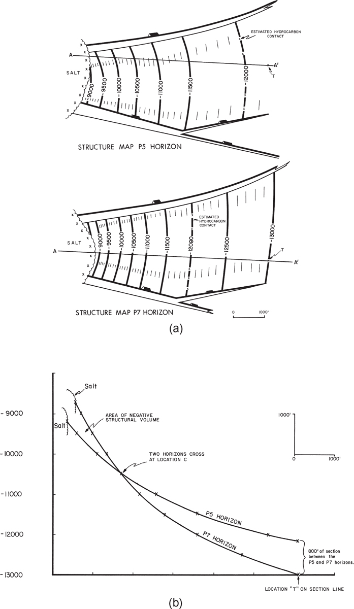
Figure 6-11 (a) Completed structure maps on the P5 and P7 horizons. These two horizons bracket a prospective section trapped by salt to the west and faults to the north and south. (b) Structure cross section prepared from the completed structure maps on the P5 and P7 horizons. The cross section clearly indicates that the completed structure maps were not constructed correctly.
Based on a study of the growth activity of a salt dome on the west, it was evident that the salt mass was a positive feature during the time of deposition of the prospective section. So the section between the P-5 and P-7 horizons should thin in the up-structure position to the west, and it does. The stratigraphic thinning was incorporated into the structural picture, but because care was not taken during the mapping process, the two structure maps depict the two mapped horizons not only converging but actually crossing up-structure. The detailed cross section of the P-5 and P-7 horizons in Figure 6-11b shows the effect of this mapping bust very clearly. Notice that the two mapped horizons intersect at the location marked C and then cross, creating a negative structural volume, which is an impossible geological situation. This mapping bust is due to carelessness in not using the technique of underlaying the completed P-5 structure map when constructing the P-7 map. Such a mistake can put a question in the minds of management as to the reliability of the work and jeopardize what might otherwise be a great exploration prospect. The preparation of a quick cross section would have caught this mapping bust.
A precise finished illustration cross section can identify many mapping problems and provide the time to correct the work before the final interpretation and maps are prepared. Also, these cross sections are excellent aids for reviewing the possibility of juxtaposed reservoirs across a fault (Fig. 6-10). Studies of such sand occurrences are important in evaluating the possibility for cross-fault drainage from one fault block to another (Smith 1980). Another type of cross section used for evaluation of juxtaposition across a fault is described in the section Fault-Seal Analysis.
Correlation Sections
In this segment of the chapter, we discuss a special type of cross section called a correlation section. This section is a special type of stratigraphic cross section that is primarily used as a detailed correlation aid. There are several important guidelines helpful in preparing this type of section.
Choose a stratigraphic datum that best serves the intended purpose of the correlation cross section (see Fig. 6-7). A reliable shale marker is usually a good choice for a stratigraphic datum (Sneider et al. 1977).
Limit the section to a short vertical log interval in order to show significant correlation detail.
Position the logs as closely as possible with no horizontal scale to include as many logs as needed in the section.
A correlation section can serve as an excellent correlation aid in defining the lateral and vertical continuity of permeable units within a specific area and stratigraphic interval. These sections can also be used as good prospecting tools to evaluate and illustrate the potential for hydrocarbons.
Figure 6-12 shows the layout for a typical correlation section. The actual electric log showing all the curves can be used; however, to reduce clutter and provide sufficient space for the inclusion of many logs, the spontaneous potential (SP) or gamma ray (GR) and the amplified resistivity curves are often sufficient. As mentioned in Chapter 4, the amplified resistivity curve is usually the most helpful for correlation work. This discussion of layout and correlation procedure applies to both manually prepared and computer-based correlation sections (see the section Cross-Section Construction Using a Computer).
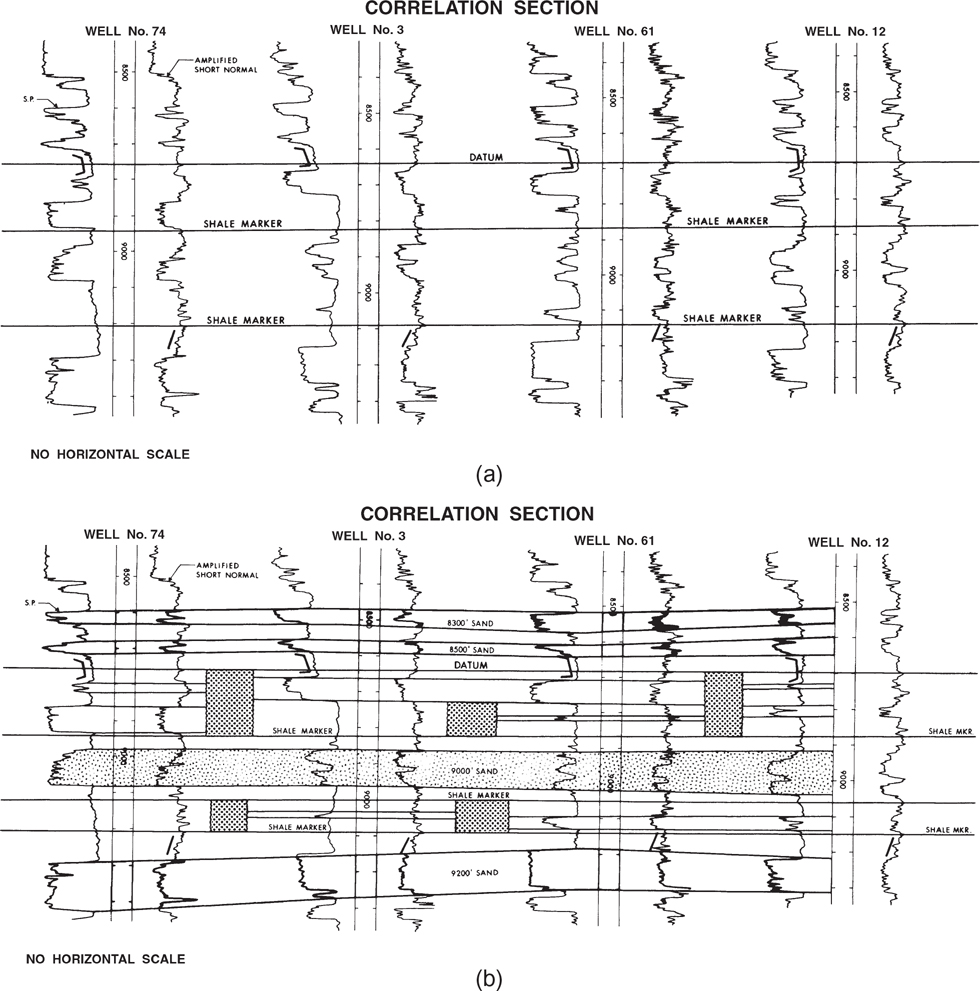
Figure 6-12 (a) Correlation section is first laid out by hanging the logs on a reference datum and correlating all recognizable shale markers. (b) Completed correlation section shows the lateral and vertical continuity (or lack of continuity) of the individual sands seen in each well.
In preparing a correlation section, follow the same correlation procedures outlined earlier in Chapter 4. Since a correlation section is a type of stratigraphic section, hang it on a well-defined datum such as the one shown in Figure 6-12a. Next, correlate the shale sections using all correlatable shale markers indicated by the SP and resistivity curves. Figure 6-12a shows the shale correlations for this section. Observe the parallel to semiparallel trend of the shale markers, which indicates a fairly uniform stratigraphic thickness. A time-stratigraphic framework now exists within which you can correlate permeable units. We use sands in this example.
We begin the sand correlations as shown in Figure 6-12b. As can be seen, the sands are not as vertically and laterally continuous and uniform as the shale sections. Lateral changes in depositional environment can cause sudden variations in sand thicknesses even within an area of limited lateral extent. Because the clays and silt that make up the shales are usually deposited in quiet waters over large areas, abrupt changes in stratigraphic thicknesses in shales are not common. Such extensive and consistent deposition of shale usually provides for good lateral correlation continuity from well to well.
The 8300-ft, 8500-ft, and 9200-ft Sands are separated vertically from the other sands, but they appear laterally continuous from well to well. The stippled pattern for the 9000-ft Sand is representative of the rest of the section. Within this overall gross sand interval are several distinct sand members in three of the wells. Based on this correlation section, it is speculative whether there is vertical or lateral continuity of individual sand members from well to well. As for the other individual sands shown in each log, they appear to be laterally discontinuous from well to well, indicating rapid changes in depositional environments and laterally limited sand bodies. The rectangular areas between wells represent discontinuity of sands somewhere between the wells.
This type of information regarding the continuity of sands is most important to the development geologist and reservoir engineer. The layout of one such section or a number of sections can often aid in making critical decisions, such as the following:
Which well or wells must be perforated to maximize the drainage efficiency within a reservoir?
Which sand interval or intervals should be perforated within a single wellbore to optimize hydrocarbon recovery?
Is a specific reservoir competitive with an adjoining lease operator? In other words, can another operator’s well on an adjacent lease drain your reserves because of possible lateral continuity of sands across the lease? If so, what action must be taken to protect your reserves?
Are any additional development wells required to optimize field production?
Can remaining reserves, identified in an abandoned well, be recovered with other existing wellbores? By this we mean, is there continuity of the hydrocarbon sand from the location of the abandoned well to a well capable of being completed?
We mentioned earlier that correlation sections can be used as an excellent exploitation tool. Figure 6-13 shows part of a geological and engineering prospect package designed to justify the drilling of a development oil well into what was considered a depleted/nonproducible oil reservoir.

Figure 6-13 (a) Structure map on the top of the 9300-ft (hydrocarbon-bearing) Sand trapped upthrown to Fault A. (b) Net sand isochore map of the 9300-ft Sand delineating the limit of good quality major sand development. (c) A detailed correlation section through the 9300-ft Sand Reservoir trapped upthrown to Fault A. The section clearly illustrates that the upper transgressive member, the fringe complex, and the channel sand are separate and distinct members of the 9300-ft Sand package. Production data indicate minor oil production from Well No.10 and that the transgressive member perforated in Well No. 4 pressure depleted (it is a closed system separated from the main 9300-ft Sand by a continuous shale break).
Figure 6-13a is a structure map on the top of a prospective sand called the “9300-Foot Sand.” An oil reservoir is present upthrown to Fault A. Six wells penetrated the oil reservoir with Wells No. 4 and 10 having produced minor amounts of oil and gas. Due to the minimum amount of oil production from Well No. 10 and the minimum gas production and pressure decline in Well No. 4, the reservoir was considered depleted. However, further study, with the use of detailed maps, log correlations, perforation data, production data, and the correlation section A-A′ (Fig. 6-13c), revealed that the reservoir consisted of three distinct sands: (1) a small, highly calcareous fringe complex, such as that seen in Wells No. 7 and 10; (2) a major cut-and-fill channel sand seen in Wells No. 3 and 4; and (3) an upper transgressive sand member separated from the fringe and channel sands by a shale break. This transgressive sand member is seen in all wells.
The correlation section (Fig. 6-13c) shows that the oil production in Well No. 10 was from the small fringe complex, and the gas production in Well No. 4 from the upper transgressive sand member. Reserves were calculated volumetrically, from net sand and net hydrocarbon isochore maps, and they were quite large compared to the actual oil and gas production. This suggested that the fringe complex and transgressive sand are separate members not in communication with the main channel sand (see delineation of major channel sand on the structure map [Fig. 6-13a], shown as a permeability barrier, and on the net sand map [Fig. 6-13b], highlighted as the limit of major channel sand). Therefore, significant reserves remain to be produced in this channel sand, which can be recovered by a recompletion in Well No. 3, if possible, or through the drilling of a new well. This prospect used the correlation section as an integral part of the prospecting process, as well as a final illustration to present the idea to management.
Cross-Section Design
In this section, we discuss the specific procedures for laying out cross sections. We review the layout of sections for four different tectonic settings: (1) extensional (normally faulted), (2) diapiric salt, (3) compressional (reverse or thrust faulted), and (4) strike-slip fault settings.
Before reviewing the section design for the four different tectonic settings, we summarize some design guidelines for cross sections.
Cross sections can be run from well to well in a zigzag pattern or as a straight line with data from each well not on the line projected into the line of section. Both types of sections have inherent problems. Zigzag sections tend to distort the subsurface geology due to changes in the strike direction of the section. If you treat a zigzag section as a series of two well straight sections, interpretation problems can be minimized. Straight-line sections may require the projection of well data over long distances, resulting in well projection problems. If you understand the various methods and limitations of projecting well data, however, straight-line sections can be used very effectively.
Deviated wells can be included in a cross section if the line of section runs along the plan view path of the deviated well (Fig. 6-15).
If a line of section being laid out intersects two closely spaced wells, include the well that penetrates the deepest section if the total depths are significantly important. Spacing may not be the critical factor; instead, similar structural geometry may be critical. In such cases, if two closely spaced wells reflect different geometry, choose the well that illustrates the geometry expected in the cross section.
When preparing both strike and dip sections in the same field, it is good practice to tie the sections together with a specific well placed on both sections (Fig. 6-14).
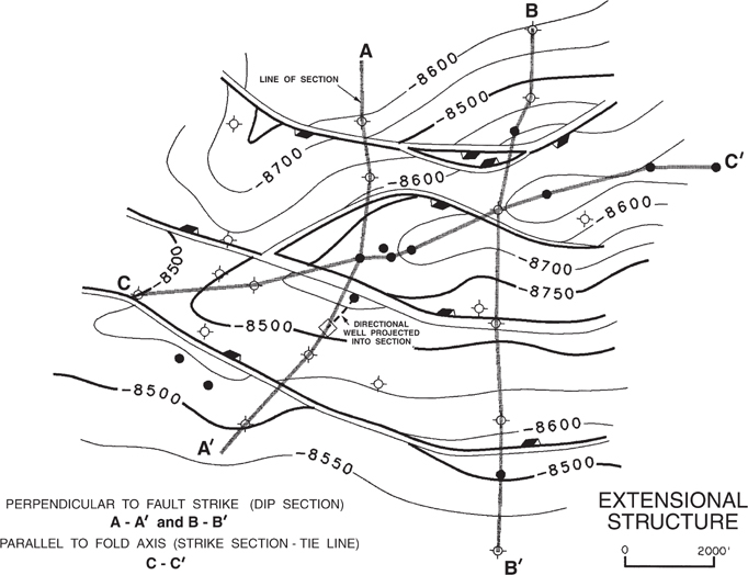
Figure 6-14 Typical layout of cross sections in an extensional tectonic setting. (Map was computer-drafted.)
Use common sense in laying out all sections. Remember, a cross section is intended to help you visualize the structure in three dimensions, give you another perspective view of the structure, and serve as an aid in solving a variety of problems related to general correlations, fault geometry, or the structural interpretation.
Extensional Structures
Figure 6-14 shows the layout for two dip sections and one strike section for a typical extensional structure. The dip sections, which are perpendicular to the strike of the faults, provide the best information for studying the faults. For single fault systems, these sections can be balanced to help develop the best structural interpretation. Sections involving bifurcating or compensating fault systems are difficult to balance due to out-of-the-plane motion, which is often difficult to account for in balancing (see Chapter 11). Initially, the cross sections can be used as problem-solving sections to help delineate the fault and structural geometry for the area under study. At the initial stages of the geological study, the straight-line method of construction for faults, horizons, salt bodies, unconformities, and other features is recommended. During the later stages of mapping, the sections can be upgraded or revised to help develop and illustrate the final interpretation. Also, cross sections such as section A-A′ in Figure 6-14 can be useful in resolving possible correlation problems in deviated wells.
Diapiric Salt Structures
Diapiric salt structures are in general structurally complex and therefore often require the layout of a number of sections to develop a reasonable geological interpretation. For an example of the cross-section design, we use the salt structure shown in Figure 6-15. A typical cross-section layout must be designed to incorporate both straight and deviated wells, since both types are commonly drilled on these structures. There are two basic directions for the cross sections: (1) strike sections (sometimes referred to as peripheral sections), which parallel or semiparallel structural strike, and (2) dip sections (sometimes referred to as radial sections), which parallel structural dip. For salt structures, we recommend that dip sections be constructed to continue past the last up-dip well control to include the salt in the cross section (see sections C-C′ and D-D′ in Fig. 6-15).
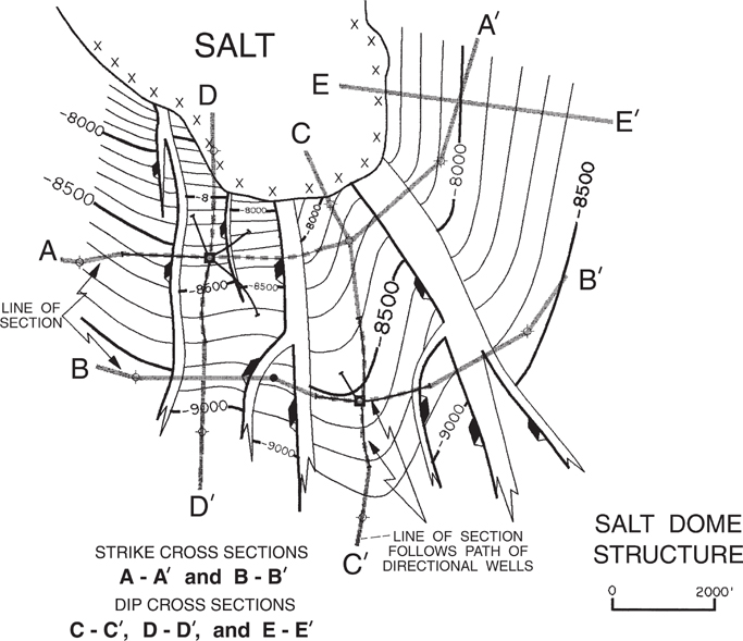
Figure 6-15 Typical layout of cross sections for a complex piercement salt structure including both straight and vertical wells. (Map was computer-drafted.)
For the structure in Figure 6-15, we show the layout of two strike and three dip cross sections. Due to the nature of the structure and the position of the wells, there is only one straight-line section, E-E′. All other sections have a zigzag pattern. The actual procedure for laying out the sections is the same as that outlined in the previous section. Observe how each line of section that includes a deviated well follows the path of that deviated well from the surface to total depth. The portion of the line of section that follows a deviated well path is dashed on the figure for clarity.
Once the structural interpretation is complete, the sections can be upgraded to serve as displays to illustrate the final interpretation. The structure maps represent the horizontal view and the cross sections show the vertical view of the 3D geometry of the structural interpretation.
Look at sections A-A′ and B-B′ in Figure 6-15. With these sections, the general fault geometry in the southern portion of this field can be studied because the sections are laid out roughly perpendicular to the strike direction of the faults. These sections are actually laid out perpendicular to the fault traces, not the strike of the faults themselves. As discussed in Chapter 8 (e.g., Fig. 8-32), fault traces can differ significantly from the strike of a fault if beds are steeply dipping, as they frequently are near salt domes. These sections can also be used to study the juxtapositioning of sands to evaluate the possibility of cross-fault drainage. The cross sections C-C′, D-D′, and E-E′, which are dip sections, provide information on the correlations, structural dip, sediment/salt interface, growth characteristics of the structure, and data on the down-dip extent of any hydrocarbon accumulations.
Finally, notice that section E-E′ is laid out with no well control. This section may be important in evaluating the structural interpretation developed for the eastern flank of the field. Such a section is constructed using the detailed illustration cross-section techniques discussed earlier. It is constructed solely from completed structure, fault, and salt maps.
Compressional Structures
The most common hydrocarbon trap in compressional areas is found in hanging wall anticlines, which form as a direct result of thrust faulting and include such structures as fault propagation folds, fault bend folds, and duplexes (Chapter 10). The anticlines commonly exhibit an asymmetry with steep frontal limbs and elongated longitudinal axes (B-axes) perpendicular to transport direction. In order to study the internal geometry of these plunging compressional folds, cross sections are normally laid out perpendicular to the B-axis (i.e., parallel to transport direction).
Figure 6-16 is a structure map on top of the Upper Triassic Nugget Sandstone in the Painter Reservoir and East Painter Reservoir Fields. Cross sections A-A′ and B-B′ shown on the map are laid out parallel to transport direction and perpendicular to the strike direction of the thrust faults. In compressional settings it is best to construct straight-line sections and plunge-project well data into the line of section to preclude the possibility of physically moving structural geometry within the fold. Such a section will also provide the best information for studying the thrust faults and balancing the structural interpretation.

Figure 6-16 Cross-section layout for a typical compressional structure. Structure map is on the Upper Nugget Sandstone in the Painter Reservoir and East Painter Reservoir Fields, Wyoming. (Modified from Lamerson 1982. Published by permission of the Rocky Mountain Association of Geologists.)
Strike-Slip Faulted Structures
The cross-section layout for structures associated with strike-slip faults is basically the same as discussed in the previous section. Strike-slip fault systems are commonly associated with faulted or unfaulted elongated anticlines. If we wish to study the geometry of an associated anticline, dip cross sections must be laid out perpendicular to the elongated fold axis. It is also recommended to tie the dip sections with at least one strike section laid out parallel or subparallel to the axis of the fold.
Figure 6-17 shows a strike-slip fault system with associated faulted anticlines on either side of the strike-slip fault. Cross sections A-A′ and B-B′ are laid out perpendicular to the fold axes. These sections can be constructed as zigzag sections in which the section line passes through each well, or as straight-line sections with the well data projected into the line of section. Cross section C-C′ is the tie line to sections A-A′ and B-B′. If internal faults such as those shown in Figure 6-17 exist on the structure, cross sections perpendicular to the fault can help in the evaluation.
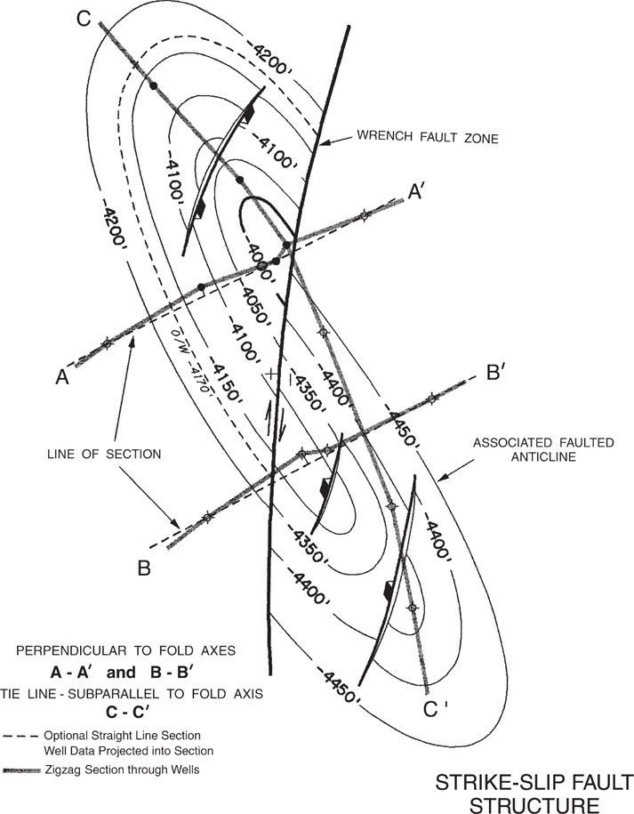
Figure 6-17 Cross section layout for a strike-slip fault system with associated faulted anticlines.
Vertical Exaggeration
Earlier in this chapter, we mentioned that, whenever possible, cross sections should be constructed using the same horizontal and vertical scales (true-scale sections). Special considerations may require that a section be prepared with different (exaggerated) scales, particularly when constructing large regional or semiregional sections. Typically, it is the vertical scale that is exaggerated. Vertical exaggeration can be incorporated into both structural and stratigraphic cross sections. Keep in mind that with the use of a vertically exaggerated scale comes various types of distortion, such as that of stratigraphic unit thickness and dip angles of horizons and faults.
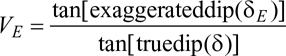
The degree of vertical exaggeration is defined as
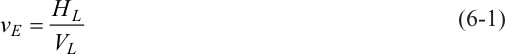
where
VE = Vertical exaggeration
VL = Length of unit distance on the vertical scale
HL = Length of unit distance on the horizontal scale
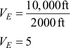
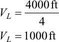
Say, for example, that you wish to prepare a cross section with a horizontal scale of 1 in. = 10,000 ft and a vertical scale of 1 in. = 2000 ft. By using Eq. (6-1), the vertical exaggeration for this cross section is
If a map has a horizontal scale of 1 in. = 4000 ft and you wish to prepare a cross section with a vertical exaggeration equal to 4, Eq. (6-1) can be rearranged to determine the vertical scale required for this exaggeration.

Therefore,
We mentioned at the beginning of this section that there are certain situations in which a cross section with a vertical exaggeration is required; in fact, it may have some advantages over a cross section with equal scales. Several situations that may require a cross section with a vertical exaggeration are (1) the preparation of a cross section in an area of low structural relief, (2) the construction of a section in an area of gently dipping beds, (3) a section that would be unreasonably long with equal scales, or (4) the need for extensive vertical detail. Consideration must also be given to the cost and size limitations of available reproduction equipment. Figure 6-18 shows two cross sections across the Uinta Basin, Colorado, which are the same except for scales. The upper section has a vertical exaggeration of 12; the lower section is true scale with the same horizontal and vertical scales. Notice how much detail can be shown on the upper, vertically exaggerated cross section as compared to the true-scale cross section.
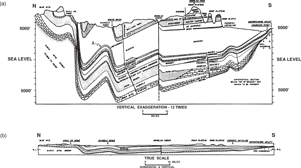
Figure 6-18 (a) A generalized cross section across the Uinta Basin, Colorado, showing the effect of vertical exaggeration (12 times). (b) Same general cross section constructed to true scale. (Modified from Suter 1947; AAPG©1947, reprinted by permission of the AAPG whose permission is required for further use.)
When a cross section is prepared with vertical exaggeration, the dip angle of beds, faults, or any other line is exaggerated. The exaggerated dip angle is not simply the product of true dip multiplied by exaggeration. Equation (6-2) defines the relationship between the true dip and the exaggerated dip (see Dennison 1968; Langstaff and Morrill 1981).
Therefore,
Using Eq. (6-2), the exaggerated dip for any cross section can be calculated if the true dip and vertical exaggeration are known. Likewise, if the exaggerated dip and vertical exaggeration for a horizon or fault are known, the true dip can be calculated. Figure 6-19 is a graphic representation of Eq. (6-2) from Langstaff and Morrill (1981). We can look at an example to illustrate the use of the graph. Referring once again to Figure 6-18, the Dakota Formation has a dip of 50 deg at location A, and the cross section has a vertical exaggeration of 12. By entering the graph on the X-axis at 50 deg, representing the exaggerated dip of 50 deg, and entering the Y-axis at 12, representing the vertical exaggeration, the intersection of the two lines generated from these data points indicates a true dip of 5.7 deg. You can see by this example that there can be significant exaggeration of dip on a cross section with a large vertical exaggeration.
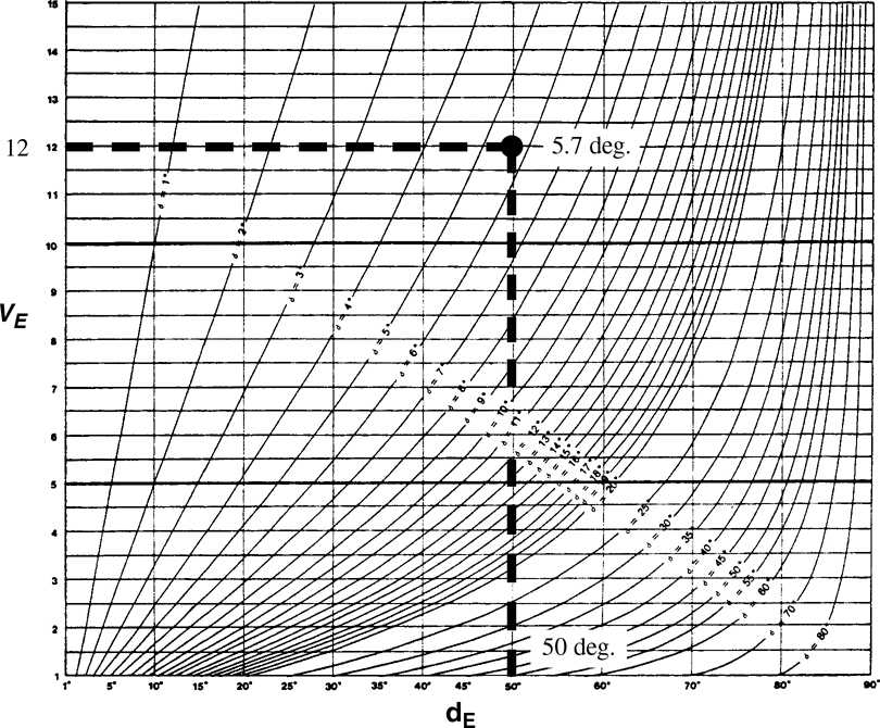
Figure 6-19 Solutions to Eq. (6-2) for different values of VE (vertical exaggeration), and (true dip). True dip occurs where VE = 1. (From Langstaff and Morrill 1981. Published by permission of the International Human Resources Development Corporation Press.)
As pointed out earlier, thickness of stratigraphic units is also affected by vertical exaggeration. If we consider that the exaggeration in the vertical direction on a cross section is a function of Eq. (6-1), it becomes apparent that interval thickness in cross section varies as a function of the exaggerated dip. Figure 6-20 shows two cross sections. Figure 6-20a is plotted true to scale and shows a unit of constant thicknesses “T.” Figure 6-20b shows the effect on the unit’s thickness with a vertical exaggeration of two. Notice that in the area of low dip, the thickness of the interval increased by a factor of two. In the area of steep dip, the interval thickness has been attenuated as a result of the exaggerated scale. It is interesting to note, however, that even though the apparent true bed thickness (stratigraphic thickness) is attenuated in the area of steep dip, the vertical thickness is still increased by a factor of two. This effect can also be seen in Figure 6-18 across the Uinta Basin. In the area of Rangely Dome, we see the effect of attenuation of the units on the flanks of the dome and the apparent thickening of the units over the crest of the structure and in the synclines on each side of the dome. In the preparation and review of cross sections with vertical exaggeration, be sure to keep such thickness changes in mind.
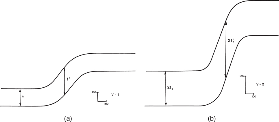
Figure 6-20 (a) is constructed to true scale. (b) shows apparent attenuation due to vertical exaggeration. Attenuation is greatest where true dip is steepest. Notice in the area of steep dip that, although the stratigraphic thickness is attenuated, the vertical thickness is twice the vertical thickness of that shown in (a), which is drawn with a true scale. (Modified from Langstaff and Morrill 1981. Published by permission of the International Human Resources Development Corporation Press.)
The decision to use vertical exaggeration in the construction of a cross section must be based on the scale of the section and its intended use. Employed wisely, vertical exaggeration can be a very useful tool. Finally, we emphasize that the use of both a vertical and horizontal graphic scale is necessary in all constructed cross sections, whether they are true scale or incorporate some type of exaggeration.
Projection of Wells
It is best to construct straight cross sections directly through wells; however, for various reasons this may not be possible, so it sometimes becomes necessary to project a well into a line of section. There are several ways in which a well can be projected into a line of section (Fig. 6-21). These include

Figure 6-21 The five most common methods of projecting well data into a line of section include (1) plunge, (2) strike, (3) up-dip or down-dip, (4) normal-to-the-section-line (minimum distance), and (5) parallel to fault. (Modified from Brown 1984a. AAPG©1984, reprinted by permission of the AAPG whose permission is required for further use.)
Plunge projection
Strike projection
Up-dip or down-dip projection
Normal-to-the-section-line projection (minimum distance method)
Parallel-to-fault-strike projection
All these methods can be used to project well data into a cross section. The best method to use, however, depends on various factors, including (1) the structural style of the area being worked, (2) the orientation of the section to the axis of the structure, (3) the horizontal distance of a well from the line of section, (4) whether there are faults on the section line, and (5) the general dip of the structure. The most commonly used methods for projecting wells into a line of section constructed by hand are the plunge and strike projections. As discussed later in this chapter, the most commonly used method of projecting wells into a line of section constructed on a computer is the normal-to-the-section-line.
Plunge Projection
In structural settings such as compressional fold-and-thrust belts containing plunging structures, the preferred method for projection of well data into a line of section is parallel to the B-axis of the fold in the hanging wall, either up-plunge or down-plunge. Figure 6-22 is a map view of a cylindrical fold. The longitudinal or B-axis of the fold is shown as B-B′, which is coincident with the axial line (Brown 1984a). The dashed lines represent plunge lines (fold elements) which are, by definition, parallel to the B-axis in a cylindrical fold. Notice that the dip rates are the same along each individual fold element, including the axial line. This is true only where the plunge rate is constant for the portion of the fold depicted.

Figure 6-22 Map view of a plunging cylindrical fold. The longitudinal fold axis (B-axis) is shown as B-B’ The dashed lines represent plunge lines that parallel the B-axis. (Modified from Brown 1984a. AAPG©1984, reprinted by permission of the AAPG whose permission is required for further use.)
One of the main objectives in plunge-projecting well data into a line of section is to preclude the possibility of physically moving structural geometry within the fold. By definition, a cylindrical fold is one in which all fold elements are parallel to one another and to the B-axis, which is parallel to the direction of plunge. A good way to visualize this is to equate a cylindrical fold to a cylinder of pipe. The edges of the pipe represent fold elements and are parallel to one another for the entire length of the pipe. Thus, the shape of the pipe’s cross section is the same at each end and everywhere in between. Similarly, a cylindrical fold contains fold elements that are everywhere parallel, and the cross-section geometry is the same throughout the length of the cylindrical portion of the fold. Therefore, projection of fold geometry into cross section A-A′(Fig. 6-22) along a line that is not parallel to the plunge lines (e.g., sides of the pipe) would result in the attempted physical movement of geometry to an improper position within the fold (e.g., projection of a 38-deg dip from plunge line No. 6 to plunge line No. 5, which has only 24 deg of dip).
We now consider the application of plunge projection. Figure 6-23 is a structure map of a plunging cylindrical fold cut by a reverse fault. We want to construct cross section A-A′ as shown on the structure map. As only Wells No. 1 and 7 actually lie on the line of section and we wish to include more data than that available from the two wells, we have no choice but to project the additional wells into the line of section.
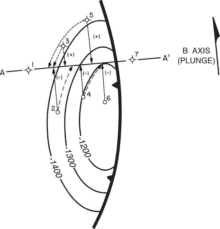
Figure 6-23 Structure map of a plunging cylindrical fold cut by a west-dipping reverse fault. (From Brown 1984a. AAPG©1984, reprinted by permission of the AAPG whose permission is required for further use.)
Well No. 1 is drilled off the flank of the structure and Well No. 7 is in the footwall in the opposite fault block. Wells No. 2 through 6 can be projected into the line of section in several different ways: most commonly, either parallel to structural strike (dashed arrow lines) or parallel to plunge (solid arrow lines). In the former case, Wells No. 2 through 5 are projected into A-A′ along structural strike (parallel to the contours), and Well No. 6 cannot be projected at all. Figure 6-24, the cross section obtained by projection along structural strike, is obviously very confusing and results in an unreasonable depiction of the fault shape, as well as the relationship of hanging wall and footwall rocks.
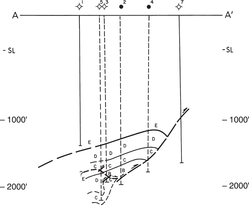
Figure 6-24 Structural interpretation along cross section A-A′ (Fig. 6-23) based on strike-projecting well data into the line of section. The strike-projected data results in an unacceptable interpretation. (Modified from Brown 1984a. AAPG©1984, reprinted by permission of the AAPG whose permission is required for further use.)
The direction of plunge of the B-axis is indicated on the structure map in Figure 6-23 to show the direction in which the wells must be plunge-projected. The B-axial direction can be obtained by analysis of any form of dip data. The solid arrows show the planned projection path of the wells into the section. Next to each projection is a + or − sign. These signs indicate whether the structural elevation for a specific horizon or structural marker (fault, dip rate, etc.) in the wells must be adjusted positively or negatively for the direction and rate of plunge over the distance projected into the section line. For example, Well No. 2 has a subsea depth for the horizon of −1340 ft. When we project this well along plunge, the top of the horizon intersects the cross section at a subsea depth of −1410 ft. Therefore, the top must be adjusted downward by 70 ft to correct for the change in elevation. This correction in elevation can actually be calculated with trigonometry by using the angle of plunge and the length of the projection from the well site to the line of section. Each well must be corrected in this manner, with (+) values indicating elevations raised because the well is projected up-plunge, and (−) values indicating elevations lowered because the well is projected down-plunge.
Figure 6-25 is the completed cross section using all the data from the wells projected into the line of section parallel to plunge, or the B-axis (in the hanging wall). In order to differentiate between the wells that actually lie on the section line from those that have been projected, the wellbore stick for each projected well is dashed. Notice also that the numerical sequence of wells (1 through 7) is now in proper order.
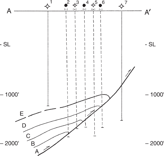
Figure 6-25 Structural interpretation along cross section A-A′ (Fig. 6-23) based on the well data projected into the line of section parallel to plunge of the B-axis. The projection of data along plunge provides the most accurate method of projecting the fold geometry into the cross section. (Modified from Brown 1984a. AAPG©1984, reprinted by permission of the AAPG whose permission is required for further use.)
In conclusion, for plunging folds, the plunge-projection method offers the most accurate means of projection of structural geometry for the hanging wall block into a cross section. This projection may be up-plunge or down-plunge, or both, and structural elevations likewise are adjusted up or down. The projections are made in order to ascertain the true cross-sectional shape of the structure.
Strike Projection
If you are mapping in a geological setting involving diapiric structures or in a tectonic area with nonplunging folds, projection along strike is often more beneficial than other types of projections. In the areas of extensional or diapiric tectonics, the dip rate on structures is typically constant along structural strike (Fig. 6-26). Therefore, in order to preserve structural geometry as well as stratigraphic relationships (syndepositional structures), wells should be projected parallel to strike.
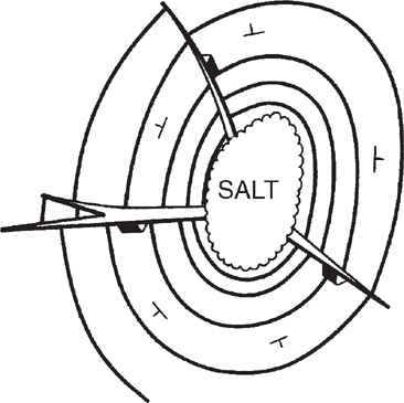
Figure 6-26 Nonplunging diapiric salt structure exhibiting constant dip along structural strike.
As you look at each example cross section, imagine each to be a seismic section into which wells are projected. Consider whether the well data would tie closely with the seismic interpretation.
We first look at an example of projecting along strike in an area without faults (Fig. 6-27). In Figure 6-27a, Well No. 2 is projected parallel to strike into the line of Section A-A′. In cross section, the M Horizon point projects into the correct structural position on the section and the rate of dip at that point would be proper for the cross section. Using this method, the projection does not require any correction factors for elevation or dip rate. In Figure 6-27b, Well No. 2 is projected along strike and again projects correctly into the line of section B-B′. We can conclude that in this type of structural situation, projection along strike is preferred.

Figure 6-27 (a) Projection of well data along strike. Upper figure is a portion of a structure contour map. The lower figure is cross section A-A′ illustrating the projected data for Well No. 2. (b) Projection of well data along strike. Upper figure is a portion of a structure contour map. The lower figure is cross section B-B′ illustrating the projected data for Well No. 2. (Published by permission of Tenneco Oil Company.)
Now we look at some examples of projecting a well along strike of a horizon cut by faults (Fig. 6-28). Figure 6-28a is a portion of a structure map showing a west-dipping structure cut by an east-dipping normal fault. East-west cross section A-A′ is plotted. Wells No. 1, 2, and 4 lie on the section line. Since data from Well No. 3 is important to the interpretation, the well must be projected into the line of section. Considering the specific geological conditions, Well No. 3 is projected parallel to strike into the A-A′ cross section, as shown below the structure map in the figure. The top of the horizon projects into the section in the correct structural position and maintains the correct structural dip, but the depth of the fault in the projected well is incorrect and must be adjusted. This adjustment is required because as Well No. 3 is projected from its actual position into the line of section, the distance from the well to the fault changes.

Figure 6-28 (a) Strike projection of well data on a horizon cut by a normal fault. The strike direction of the fault does not parallel the strike of the mapped horizon. Upper figure is the structure contour map. In the lower figure, cross section A-A′ illustrates that the well depth point for the mapped horizon fits the cross section; however, the fault location in Well No. 3 is too deep and must be adjusted. (b) Parallel-to-fault-strike projection. The well data are projected parallel to the strike of the fault surface. The fault projects correctly into the line of section, but the horizon depth must be adjusted. (Published by permission of Tenneco Oil Company.)
You might already have asked yourself the question, if the well is projected parallel to the fault, how will the fault and horizon project into the line? Figure 6-28b depicts this situation. Well No. 3 is projected into the section line parallel to the strike of the fault surface. With this projection, the fault location in the well fits the section correctly, but the horizon point is projected too shallow, requiring an elevation adjustment from −590 ft to −605 ft.
When projecting wells along strike of a horizon cut by faults, either the horizons or the faults usually will require an elevation adjustment. Therefore, we caution that projected wells often have limited use in a cross section and can, at times, cause more confusion than clarity. If a well must be projected into a line of section, be sure to identify the projected electric log or wellbore stick with a dashed line and clearly note any required corrections or adjustments.
Other Types of Projections
Figure 6-29 illustrates two other types of projection: one normal to the line of section and one parallel to the bed dip direction. Well No. 2 in Figure 6-29 is projected normal or at a right angle to the section line. This is sometimes referred to as the minimum distance method (Brown 1984a). Also, it is the typical method for projecting a well into a seismic line. Using this method for well projection, the horizon does not plot correctly on the section. In addition, it is possible that the dip of the horizon may be different at the actual well location than at its projected location on the line of section, since the well is projected into a higher structural position. This can add confusion to the section and may also require adjustments in the stratigraphic interval thicknesses in the projected well. This is the default method for projecting wells into cross sections when working on a computer.

Figure 6-29 Projection of well data into a line of section, using the normal-to-section and down-dip projection methods. Neither method is recommended for projecting well data. (Published by permission of Tenneco Oil Company.)
The second projection shown in Figure 6-29 is a down-dip projection of Well No. 4. With this projection, the horizon is projected incorrectly. Also, a problem may exist with the projected horizon dip rate, since the well is being projected into a down-dip position. Neither method is recommended for projecting well data into a cross section.
Projection of Deviated Wells
If a directionally drilled well is to be included in a cross section, it is best to have the line of section follow the plan view path of the deviated well (Fig. 6-15). If the line of section is not coincident with the well path, the well will have to be projected into the cross section. The procedure for such data projection is shown in Figure 6-30, which shows the map view of directional Well No. 6 and its projection into the line of section A-A′. The deviated well path is almost coincident with the section line, but not exactly. Therefore, directional survey data points must be projected into the line of section. This is accomplished by first determining the approximate direction of structural strike, either from a structure map or seismic data, and then projecting each data point parallel to the horizon strike direction as shown in the figure.
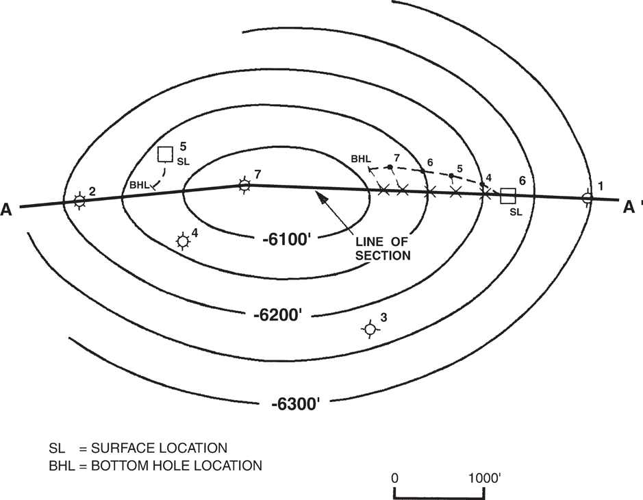
Figure 6-30 Structure contour map with line of section A-A′. Deviated Well No. 6 is projected into the line of section parallel to horizon strike.
If the electric log is represented by a stick, each directional survey data point is plotted individually in cross section and then the points are connected with a smoothly curved line representing the electric log in stick form. Notice in Figure 6-30 that the projected data points for the 4000-ft, 5000-ft, 6000-ft, and 7000-ft true vertical depths are not the same distance from the surface location as the actual depths plotted along the directional path. This correction must be made when the individual directional survey points are plotted in cross section. If each survey data point is projected correctly and plotted correctly in cross section, the projected directional wellbore stick will depict the true representation of the directionally drilled well in cross section.
When the actual electric log for a deviated well is used to project into a cross section being constructed by hand, the log must be cut at various locations to retain true vertical or subsea true vertical depth, whichever is used. In Figure 6-30, we see that the projected depth points plotted on the map are not the same distance from the surface location as the actual plotted depths. Therefore, adjustments must be made to the log in order to include it in the cross section. These adjustments are made by cutting out small sections of the log at various depths, as needed, to maintain true vertical or subsea depth on the section after projection. Computer software can display a deviated well projected onto a plane but most software does not project the deviated well along strike. In part this is because the software does not know the strike of the bed.
Figure 6-31 shows a deviated well log that is cut at various depths to retain its true depth in cross section after projection. It is best to delete sections of the log that do not contain any important correlations. If possible, shale sections should be used to make these adjustments.
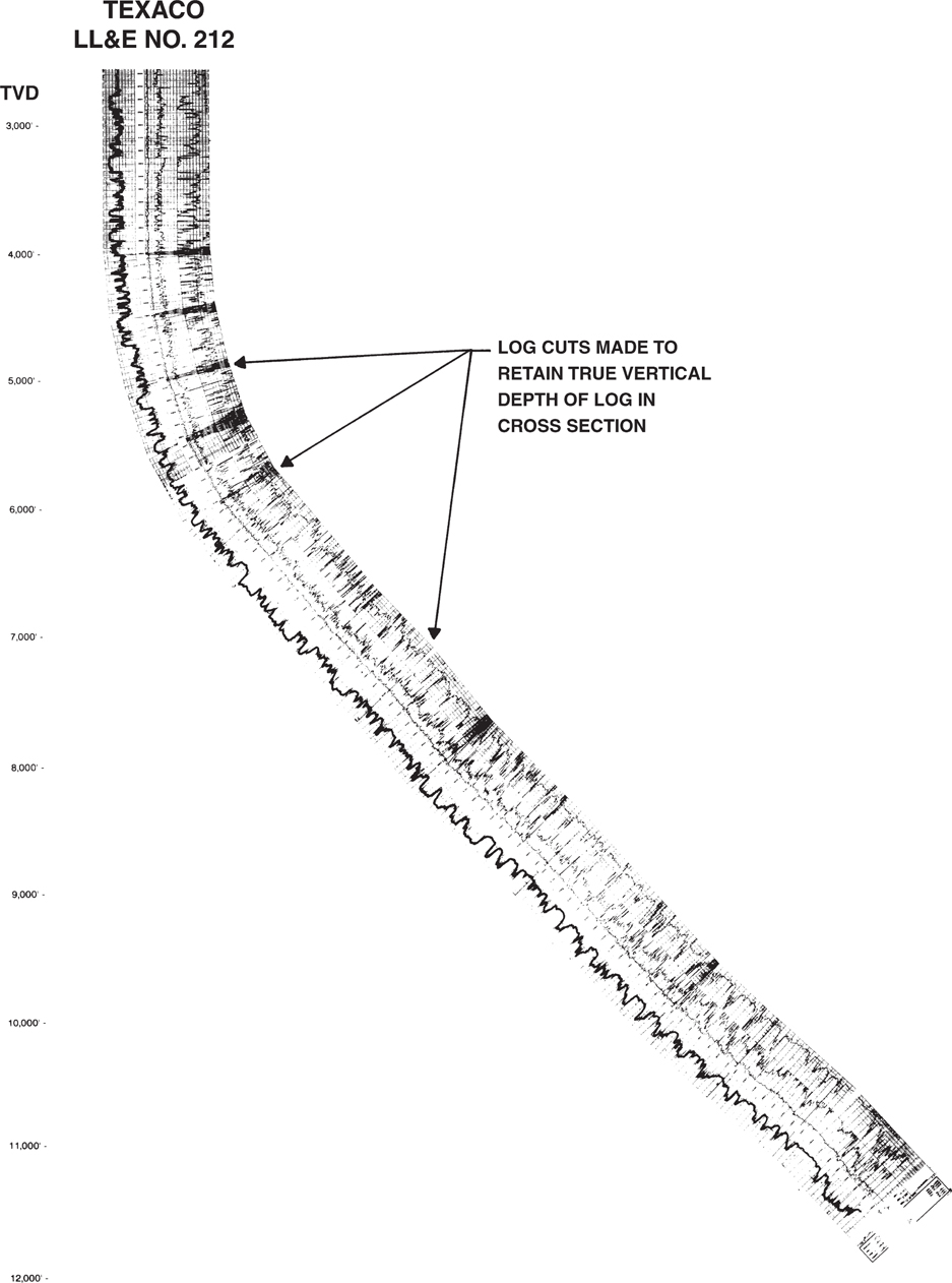
Figure 6-31 The film of the log for Well No. 212 is cut at various depths to retain true vertical depth of the entire log in cross section.
Figure 6-32 is a north-south structural cross section through West Cameron Block 192 Field, northern Gulf of Mexico. The section is composed from six vertical and six directionally drilled wells. The structure map on the U Sand is placed as an insert on the cross section. Notice that the line of section has a zigzag pattern from north to south. Apparently, this zigzag pattern was used to accommodate directionally drilled wells. In other words, the path of the section line changes direction to parallel as closely as possible the path of the directional wells. By doing so, the projection of data from each deviated well into the line of section is minimized, thereby providing the most accurate representation of the directionally drilled well data in the cross section.

Figure 6-32 North-south structural cross section in West Cameron Block 192, northern Gulf of Mexico. The section line (see structure map insert) has a zigzag pattern to accommodate the directionally drilled wells, thus minimizing the projection of well data into the line. (From Offshore Louisiana Oil and Gas Fields, v. II, 1988. Published by permission of the New Orleans Geological Society.)
Projecting a Well into a Seismic Line
A well path projected into a seismic line (Fig. 5-15a and b) can often cause more confusion than clarification to an observer unfamiliar with the projection or details of the geological structure. Off-depth projections of horizon and fault positions in wells result in a mis-tie of the seismic with the well data. Therefore, care must be taken to properly project a well into a seismic section and label clearly the projected well data. If you are working with 3D seismic data, then the creation of an arbitrary line through a well can avoid the problems of projection into a line. However, if the velocity function used to convert the well depths to time for plotting the well is inaccurate, or if the well and/or seismic lines are incorrectly spotted, then a mis-tie can still occur.
The techniques outlined for projecting a well into a cross section are also valid for projecting well data into a seismic section. The following are a few additional suggestions that may help when projecting a well into a seismic section.
Be certain that the velocity function is the most accurate one for the area. Incorrect velocity information can cause some serious errors when projecting a well, particularly if it involves a directionally drilled well. Even when working with seismic displayed in depth it is important to remember that the velocity function used to convert time seismic into depth seismic may not be completely accurate (Fig. 5-29). Also, remember that a seismic section is not a geological cross section and that the apparent angle of a well on a seismic section may not resemble the angle of the well on the equivalent geological cross section. It is also important to know both the horizontal and vertical scales of the seismic section being used.
Consider dashing all projected wells posted on a seismic section. If the well path actually crosses the plane of the line, mark the point clearly with a different color solid line or a horizontal dash across the well path. Many computer systems use this or a similar convention when projecting wells onto seismic sections.
Remember that when a well is projected along structural strike, many of the faults may appear to intersect the projected well path at different depths than the actual intersections in the well. Be ready to field questions when a line like this is used for presentation purposes.
Too often, the minimum distance (normal-to-the-line) projection method is used for projecting well data into a seismic section. Whenever possible, do not use this method, because the data frequently will be projected incorrectly, resulting in a conflict between the well and seismic data (Fig. 5-15a and b). The minimum distance projection method is the default method for projecting wells onto seismic lines for all interpretation software systems of which we are aware. Many software systems may not allow an alternative method of projection.
It is not good practice to project well data over long distances into a seismic section. Remember the geometry of any structure changes laterally even over short horizontal distances. Projections of well data over long distances can and often do cause great confusion in the interpreted seismic section.
Cross-Section Construction Across Faults
In Chapter 7 we discuss the importance of the fault component vertical separation and define the missing or repeated section in a wellbore, resulting from a fault, as being equal to this fault component. Therefore, when constructing a cross section with faults, the vertical separation must be used to correctly displace a horizon or stratigraphic unit from one fault block to another. In this section, the method for using the vertical separation in the preparation of a cross section containing a fault is discussed in detail. The concept is basic and the correct technique of construction very simple, yet the technique is often misused. Before reading this section, it may be necessary to become familiar with the fault component vertical separation and the difference between this component and fault throw. These subjects are covered in the beginning of Chapter 7, particularly in the sections titled Definition of Fault Displacement and Fault Data Determined from Well Logs.
If the missing section in an electric log is mistakenly used as throw in the construction of a cross section involving a normal fault, chances are the displacement of horizons across the fault will be incorrect. The values for vertical separation and throw are the same only for a vertical fault and for a fault that cuts through horizontal beds. With increasing bed dip, however, the values are different and can be significantly so with steeply dipping beds. Therefore, the bed displacement error in a cross section, using the missing section as throw, will usually be greater with increasing structural dip.
Figure 6-33 graphically depicts the correct method for using vertical separation (missing section) to obtain the proper bed displacement across a normal fault. The incorrect method using throw as the missing section is also shown for comparison. In this example, assume there is sufficient control from well data or a structure map in the downthrown fault block to establish the dip of the horizon (Bed A) and its intersection with Fault 1 in the downthrown block at −7100 ft, as shown in Figure 6-33a. The missing section for Fault 1 determined by log correlation is 300 ft. With this information, the next step is to determine where Bed A intersects the fault in the upthrown fault block. This is accomplished by correctly plotting the 300 ft of missing section as vertical separation across the fault into the opposite fault block. Vertical separation is defined as the measured vertical distance between a bed projected from one fault block across the fault to a point where the projection is vertically over or under the same bed in the opposite block. The missing or repeated section observed in a wellbore as the result of a fault is equal in value to vertical separation and not throw. Applying this definition to the normal fault in the cross section in Figure 6-33b, the dip of Bed A is projected from the downthrown block through the fault, as if the fault were not there, to the upthrown block until it is 300 ft vertically beneath the fault. The depth at this point on the fault (−6900 ft) is the upthrown intersection of Bed A with the fault, and Bed A is then constructed from that point.
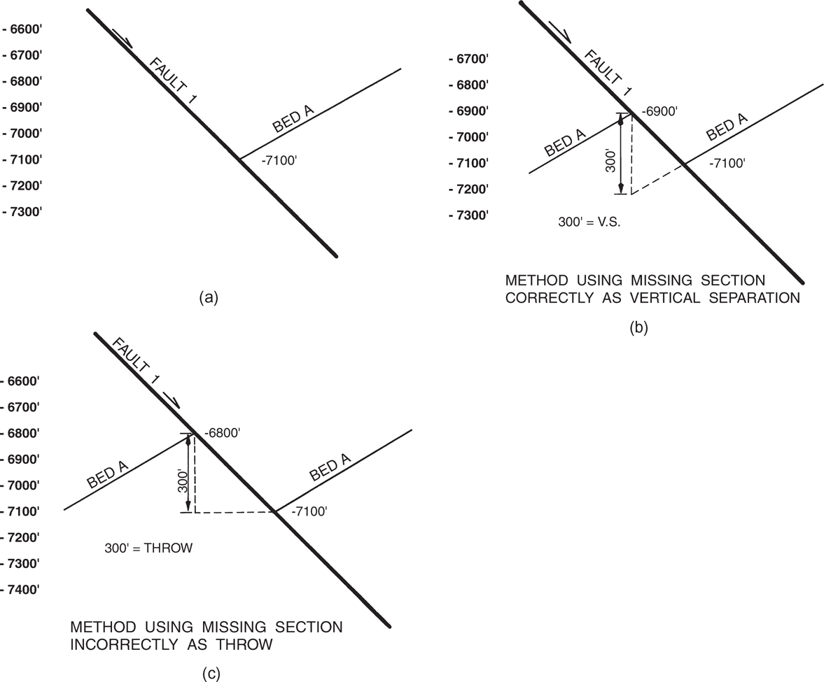
Figure 6-33 The correct method for displacing a horizon across a normal fault in cross section is to plot the vertical separation of the fault. (a) First, establish the horizon dip and intersection with the fault in the fault block with the most control; in this case, the greatest amount of control is in the downthrown fault block. (b) Plot the vertical separation to determine the depth of the intersection of the horizon with the fault in the opposite fault block, in this case the upthrown fault block. (c) An incorrect method for displacing a horizon across a fault is plotting the missing section for the fault as if it were throw. Compare results to those of the correct method shown in (b).
Now look at the missing section plotted incorrectly as throw (Fig. 6-33c). Throw is defined as the difference in vertical depth between the fault intersection with the bed in one fault block and the fault intersection with the same bed in the opposing fault block, determined in a direction perpendicular to the strike of the fault. Applying this definition to the cross section in Figure 6-33c, which is perpendicular to the strike of Fault 1, the depth of intersection of Bed A with the fault in the upthrown fault block is −6800 ft.
There is a 100-ft vertical difference between the two methods in the estimated depth of the upthrown intersection of Bed A with the fault. Incorrectly using the missing section as throw places the upthrown block 100 ft too high. This mistake could be costly, particularly if a well were planned for the upthrown block based on the incorrect interpretation, which plotted the amount of vertical separation as throw.
Using the missing section incorrectly as throw has an additional problem if the line of section is not perpendicular to the strike of the fault. Throw is measured perpendicular to the strike of the fault. If the line of section is not perpendicular to the strike of the fault, it illustrates apparent throw, which is always less than true throw (Suppe 1985). The best way to determine the strike of the fault is to map the surface of the fault as described in Chapter 7. If the missing section is used correctly as vertical separation, the orientation of the line of section relative to the strike of the fault is irrelevant as vertical separation is independent of the strike of the fault as the bed is projected across the fault using the dip of the bed along the line of the cross section.
Because this technique is so important, we will review it with two other geological examples, one involving a normal fault and the other a reverse fault. Figure 6-34 shows cross section A-A′ and an insert enlargement of a portion of the section. The missing section in Wells No. 2, 3, and 5 for the normal Fault 1 is 400 ft. The missing section is equal to vertical separation, so we use this fault component value to prepare the cross section construction across Fault 1.
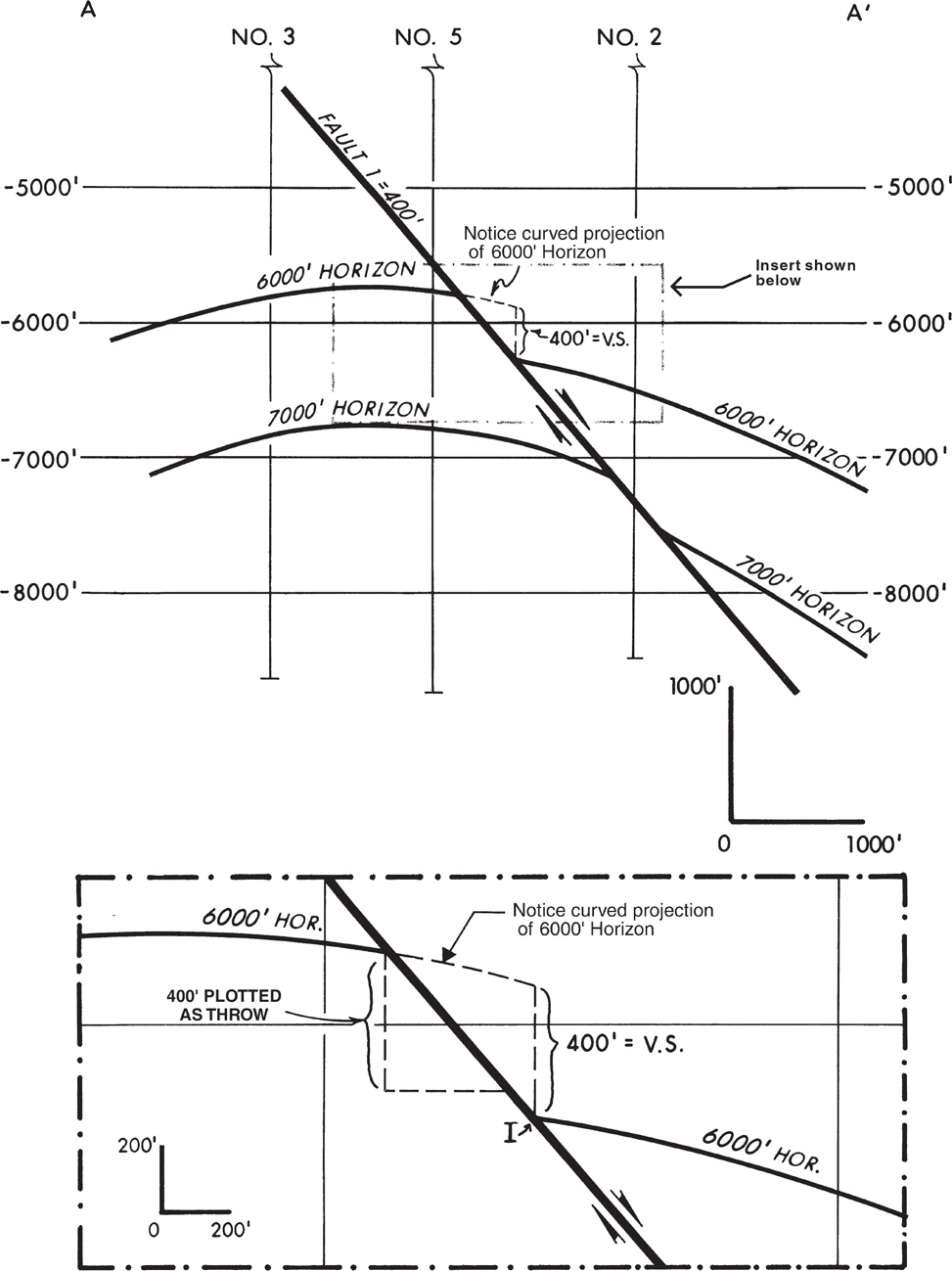
Figure 6-34 An illustration using the correct method for displacing a horizon across a normal fault.
The structural attitude of the 6000-ft horizon in the upthrown block of Fault 1 is established by using the available well control in that block and a completed structure map. Well No. 5 is sufficiently close to the intersection of the 6000-ft horizon with the fault to establish the depth at which this intersection occurs. Once this depth has been established, we must determine the position (depth) at which the horizon intersects the fault in the downthrown block. The depth chosen again depends on your understanding of missing section. You must use the definition of vertical separation to project the dip of the 6000-ft horizon from the upthrown block, through the fault as if the fault were not there, into the downthrown block until the projection is 400 ft vertically above the fault. The point labeled I in the insert is the correct intersection of the horizon with the fault in the downthrown block. Notice that the projection of the 6000-ft horizon from the upthrown to downthrown blocks is curved to follow the actual changing dip of the unit.
Remember, the missing section is not equal to throw in areas involving dipping beds. Therefore, if the mistake is made of using 400 ft of missing section as throw, then the estimated depth of the intersection of the horizon with the fault in the downthrown block would be incorrect. In this case, shown in the insert in Figure 6-34, the intersection point would be too shallow by approximately 75 ft.
We now look at one example involving a reverse fault. The vertical separation for a reverse fault is equal to the repeated section in a well cut by the fault. Figure 6-35 shows cross section A-A′ and an enlarged insert of a portion of the cross section. The repeated section resulting from Fault 1, as correlated with all surrounding well control, is 400 ft, which is the vertical separation of the fault.
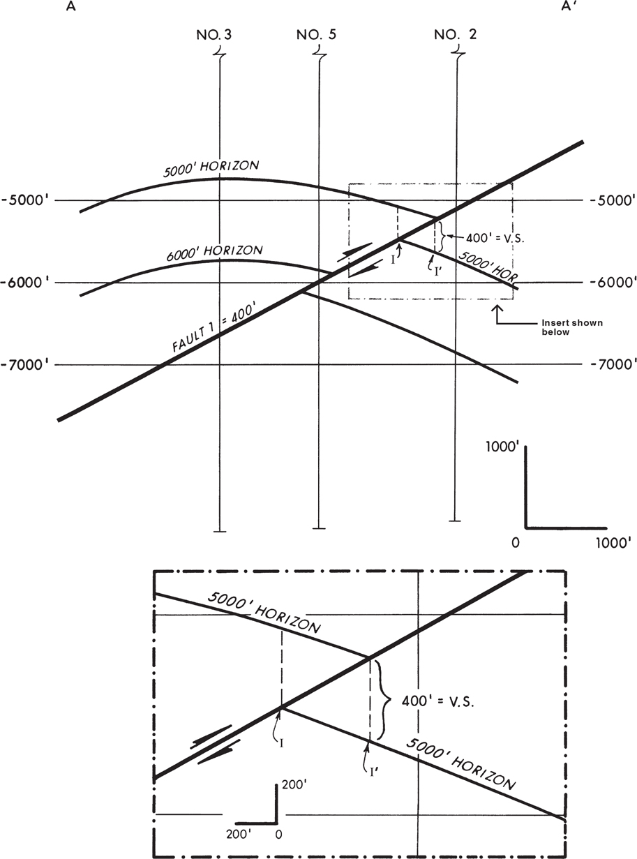
Figure 6-35 An illustration using the correct method for displacing a horizon across a reverse fault.
Assume, for this example, that due to more well control, the attitude of the 5000-ft horizon and its intersection depth with Fault 1 is first established in the hanging wall block. The task now is to determine the displaced position of the horizon in the footwall block and the depth of its intersection with the fault. With reverse fault geometry, the technique is actually easier than with a normal fault and can be used to establish two control points for the 5000-ft horizon in the opposing fault block (in this case the footwall). Working with the enlarged portion of the figure, follow along the horizon in the hanging wall until the bed is at a point that is 400 ft vertically above the fault surface. This point, labeled I, is the footwall intersection of the horizon with the fault. A second point of control for the 5000-ft horizon can be established by measuring 400 ft vertically down from the intersection of the 5000-ft horizon with the fault in the hanging wall. This point, labeled I′, corresponds to the depth to the top of the horizon in the footwall at the point vertically beneath the intersection of the sand with the fault in the hanging wall.
As an academic exercise, estimate the intersection of the 5000-ft horizon with the fault in the footwall using the incorrect assumption that the 400 ft of repeated section corresponds to the throw of the fault. As a second exercise, estimate the size of the actual fault throw considering the correct geometry shown in Figure 6-35.
It is important to note again that the preciseness of the projection of horizon dip, through a fault, determines the accuracy of the displacement across the fault. If the bed dip changes in the area where the projection is made, the projection must follow this changing bed dip (observe again the curved projection of the 6000-ft horizon in the enlargement insert in Fig. 6-34). In other words, the projection of a horizon across a fault need not be a straight line. If the bed dip is not constant across the fault, then the projection must follow the changing bed dip for you to accurately construct the vertical separation.
The precision of determining the intersection of a horizon with a fault using vertical separation is also dependent on knowing the depth of the fault along the line of section. The best way for determining the depth of the fault along the line of section is to create a structure map of the surface of the fault as discussed in Chapter 7.
Three-Dimensional Views
Many types of computer software provide 3D views of mapped surfaces and rock volumes. These are more easily generated and preferable to hand-drawn 2D representations of 3D geology. However, the latter are sometimes appropriate or necessary, so we present here some methods that help in 3D visualization of the geology.
In petroleum exploration and exploitation, a map or cross section alone cannot always represent the complete subsurface geological picture, because each is limited to two dimensions. Since neither a map nor cross section presents data in three dimensions, a detailed study may require the use of additional techniques that aid in visualizing the geology in three dimensions. Such additional aids include log maps, stick or fence diagrams, isometric projections, 3D structural models, and block diagrams.
Log Maps
Log maps are the simplest means of combining plan view information with some vertical dimensional data. Figures 6-36 and 6-37 illustrate two different types of log maps. In Figure 6-36, electric log sections and data charts for the Miocene Middle Cruse Sand Member in Trinidad are superimposed on a structure map of the same sand member. This type of map allows you to quickly review the vertical sand conditions and producing characteristics of the sand in each well with respect to the well’s structural position within the reservoir. Notice that only the SP and the amplified short normal resistivity curves were used in the log sections. By looking at this map, you can very quickly see the complexity of the one or more sand members compromising this reservoir and the relationship of sand quality to structural position and well location.
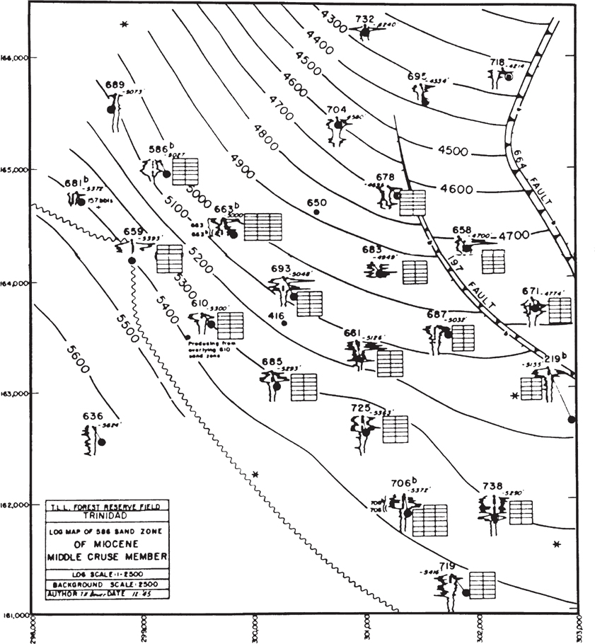
Figure 6-36 Log map of the Miocene Middle Cruse Sand Member (Trinidad). The SP and amplified short normal log curves are superimposed on the structure map of the sand. The relationship of sand quality to structural position within the reservoir can quickly be evaluated. (Modified after Bower 1947; AAPG©1947, reprinted by permission of the AAPG whose permission is required for further use.)
Figure 6-37 is another type of log map in which the SP curve for each electric log is placed next to the appropriate well location in an attempt to portray the 3D paleogeographic conditions during the time of sand deposition. In this field, the sands appear to be of two types: (1) a major cut-and-fill channel sand, and (2) a very poor-quality, highly calcareous fringe complex. The calcareous nature of the sand was determined from cores taken in a number of wells.

Figure 6-37 Another type of log map. The SP curve for each well is placed at the surface location for the well in an attempt to visualize the 3D characteristics of the 10,500-ft Sand. (Published by permission of Texaco USA.)
If the actual structure map for the 10,500-ft Sand were superimposed on this log map in a manner similar to that shown in Figure 6-36, this additional step would improve the evaluation of the sand conditions with respect to the localization of the major channel sand and calcareous fringe complex sand in comparison to the structural position of the individual wells, production characteristics of the local reservoirs, and hydrocarbon-trapping conditions. Such information can lead to the identification of overlooked workovers and recompletions, in addition to possible development drilling locations.
Fence Diagrams
Fence diagrams, also called panel diagrams, consist of a 3D network of cross sections drawn in two dimensions. They are designed to illustrate the areal relationship among several wells that are located in close proximity to each other. Fence diagrams can be either structural or stratigraphic. Figure 6-38 is a typical example of a fence diagram in which actual electric log segments have been traced for use at each well location. Fence diagrams are often prepared using only log sticks, although log sticks do not provide the correlation detail usually needed for detailed work. Fence diagrams are also usually diagrammatic because they seldom have a common horizontal and vertical scale.
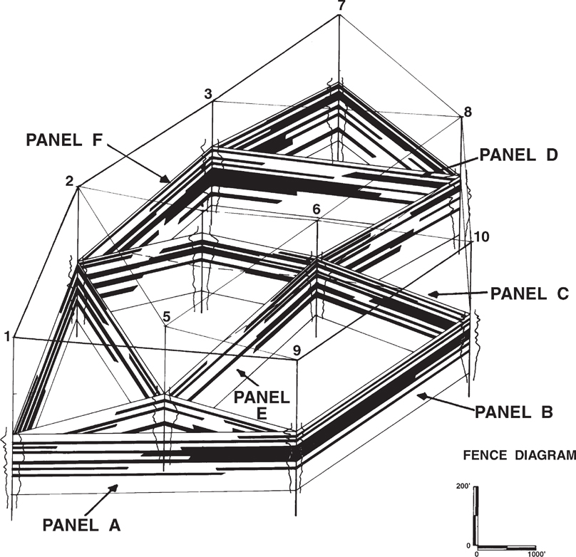
Figure 6-38 Layout of a typical stratigraphic fence diagram in which the actual electric log segment for each well was traced at the well location. (Modified from Boeckelman, unpublished. Published by permission of author.)
Fence Diagram Construction
The construction of all fence or panel diagrams begins with a well basemap. The plane of the basemap represents a chosen datum plane and each well location is taken to be the point where the well intersects the datum plane. A vertical line is drawn at each well control point and the well data are either hand-plotted along this line or a film of the actual log curves, reduced to the proper scale, is attached to the line. For example, in Figure 6-38, the SP and resistivity curves were hand-traced from reductions of the actual log. Figure 6-39 is a fence diagram constructed using the actual reduced log curves.

Figure 6-39 Layout of a stratigraphic fence diagram using the actual reduced log curves. (From Langstaff and Morrill 1981. Published by permission of the International Human Resources Development Corporation Press.)
In the preparation of a structural fence diagram, the reference plane of the map is a chosen datum, which can be sea level or any elevation above or below. For example, the chosen datum for the fence diagram in Figure 6-40 is −1500 ft, which is a subsea datum equivalent to 1500 ft below sea level. The log sections or hand-traced curves are hung on the vertical line at each well location and are referenced to the chosen datum. The structural profile of the bed(s) on the section is drawn by initially connecting the major correlation markers from each well. The number of correlation markers connected depends on the detail desired for the diagram.
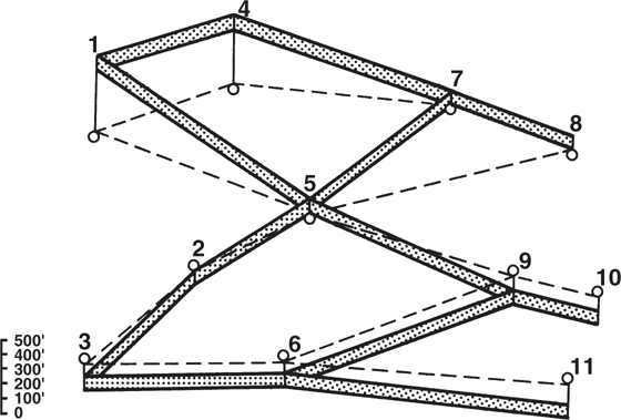
Figure 6-40 Structural fence diagram: reference plane (dashed line) is 1500 ft below sea level. (From Bishop 1960. Published by permission of author.)
It is important to try to minimize the interference of one panel with another to reduce the effect of masking data. It is a good idea to begin to complete the panels starting with the east-west sections first, and in particular, the panels nearest the lower or front end of the map (see panels A, B, and C in Fig. 6-38). The northwest-southeast or northeast-southwest panels are completed next, up to a point where they intersect the east-west panels from the front or where they disappear behind these panels from the rear, such as panels E and F in Figure 6-38. Once all the correlation markers have been connected on all the panels and the desired labeling added, the diagram is complete. If dips are most prominent in the north-south direction, an isometric projection may be more helpful, or the diagram may be drawn with north toward the right instead of toward the top of the map, as is more common.
For the construction of a stratigraphic fence diagram, the plane of the map is considered to be either the bedding plane or an unconformity that is the chosen datum horizon. Just as with the structure fence diagrams, a vertical line is drawn at each well location. Since most stratigraphic fence diagrams are prepared to illustrate correlations, facies changes, permeability barriers, sediment wedging, or some other stratigraphic feature, the actual log sections are normally required. Connect all the correlation markers to complete the fence diagram (Figs. 6-38 or 6-39).
Isometric Projections
Isometric projections are sometimes used to emphasize certain stratigraphic variations that might not be apparent on the conventionally oriented fence diagram. In an isometric projection, the map base is shown as if it were turned at an angle and tilted toward the front, which transforms the projection from orthogonal to nonorthogonal axes (Langstaff and Morrill 1981). Figure 6-41 shows the difference between a standard fence diagram and its transfer into an isometric projection. Notice that the rectangular basemap becomes a parallelogram in the isometric projection.

Figure 6-41 Comparison of (a) a standard stratigraphic fence diagram to (b) an isometric projection. (From Langstaff and Morrill 1981. Published by permission of the International Human Resources Development Corporation Press.)
The basemap used in Figure 6-41 has a coordinate grid system with both north-south and east-west scales provided. Any isometric projection will have distortion in any direction except in the directions of the original grid system. In other words, all lines parallel to the original north-south and east-west axes remain parallel in the isometric projection. Therefore, any data points to be measured from the basemap must be measured along one or both of these coordinated grids, and by doing so they can be measured accurately. Measured distances in any direction except parallel to the original grid coordinates will be distorted. They may be greater or less than the actual distance. It is very important, therefore, to always include some type of coordinate grid system on all map bases that are planned as isometric projections.
Three-Dimensional Reservoir Analysis Model
One of the most accurate and detailed types of projections is what we call a 3D reservoir analysis model, abbreviated RAM (Wayne Boeckelman, unpublished). Using the basic rules of descriptive geometry, we can construct a 3D of a structure from which true length and true slope can be measured. This is accomplished by constructing the folding plane at 90 deg to dip (Fig. 6-42).

Figure 6-42 A 3D RAM (reservoir analysis model) can be constructed to measure true length and slope by constructing the folding plane at 90 deg to dip. (From Boeckelman, unpublished. Published by permission of author.)
Construction Procedure
The construction of a 3D RAM must begin with a completed structure map such as the one shown in Figure 6-43a. Choose a grid that is 90 deg to the dip of the structure (Fig. 6-43b) so that true length and true slope can be plotted and measured from the model. Be sure that grid lines, which later become the 3D panels, go through all the wells on the structure map, as shown in Figure 6-43b, to ensure the use of all the geological control. In this example, there are six wells to include in the grid. Notice, however, that there will eventually be more control points than just those from the six well locations. The model shows that there are actually 18 grid line intersections in addition to those through the six wells. Each of these intersections serves as a data control point. This means that there are a total of 24 geological control points for the construction of this example model. You can immediately see that one of the benefits of this type model is to provide a more accurate interpretation because of the large number of control points.
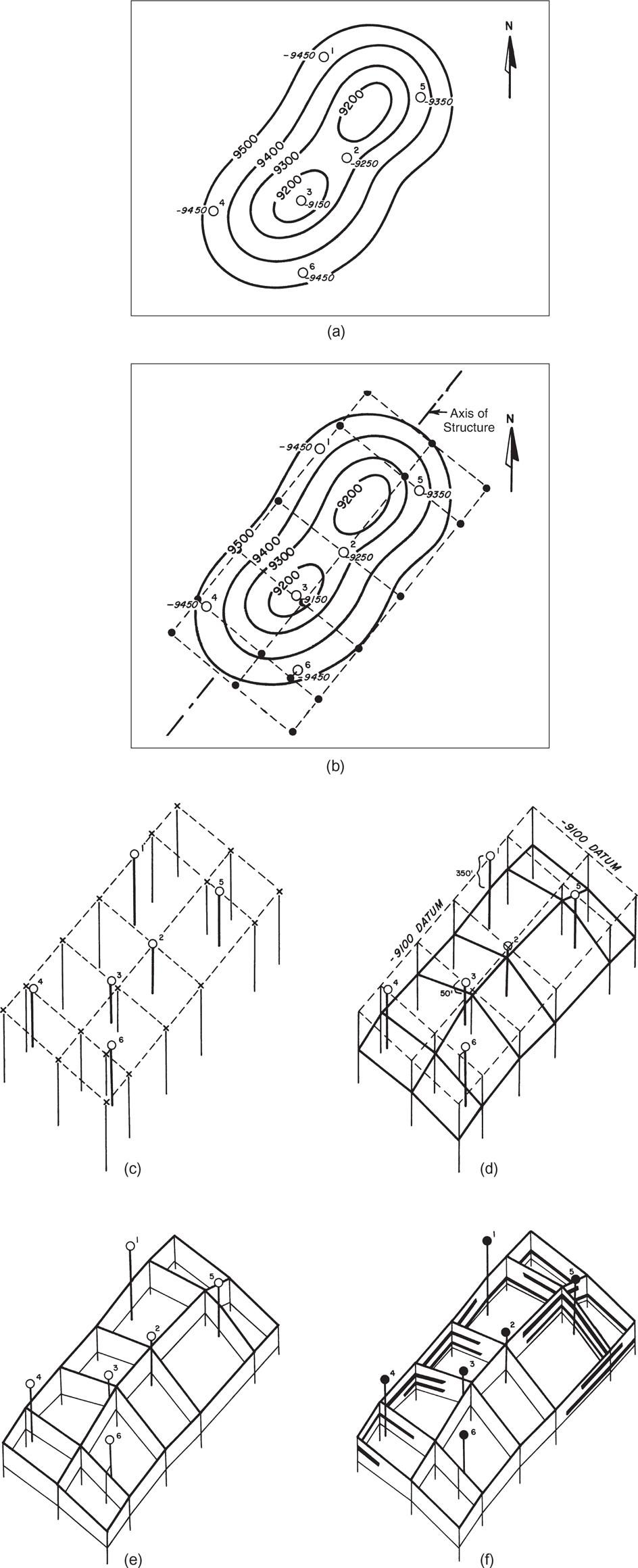
Figure 6-43 (a) Completed structure map on the top of the 9200-ft Sand. (b) RAM grid positioned at 90 deg to dip. Grid lines must intersect each well to ensure the use of all geological data. (c) Choose a datum and construct lines from the datum vertically straight down from each well and grid location. (d) Post the elevation for the top of the 9200-ft Sand at each grid intersection and connect the points with straight lines representing the top of the 9200-ft Sand. (e) Overlay the grid system on the base of the sand map and post the base of the sand at each grid intersection and each well location. (f) Begin detailed construction of the sand and shale data for each panel starting at each well location, working outward in all panel directions. (From Boeckelman, unpublished. Published by permission of author.)
Once the grid system is laid out, extend a line vertically straight down from each well and grid intersection, as shown in Figure 6-43c. As with all the other types of 3D diagrams, a datum must be chosen. For this example, we chose −9100 ft as the datum, so all data are referenced from this datum. Once the datum is chosen, we are ready to plot data for the specific stratigraphic interval to be studied. In this model we study the 9200-ft Sand.
We begin with a review of how to place the log or hand-drawn curves on the vertical line with reference to the datum. Since the intent is to evaluate the entire 9200-foot Sand package, the representation of this sand package must be placed on the model, and in doing so there are several choices. The most accurate method is to make a reduced film of the actual log section to accommodate the scale of the model and hang the log section on the structural top of the 9200-ft Sand at each well location. As mentioned before, it is best to use a limited number of log curves to reduce clutter on the model. The second choice is to hand-trace the reduced log curves on the vertical line at each well location. The choice is more a matter of preference.
Our interest, in this case, is to hang the section on the top of the 9200-ft Sand in order to study and review the entire 9200-ft Sand package. At Well No. 3, for example, the top of the 9200-ft Sand is at a depth of −9150 ft. Since the referenced datum is −9100 ft, the first depth point is 50 ft below the datum. The log or hand-drawn curve(s) is positioned so that the top of the sand is 50 ft below the reference grid at Well No. 3, as shown in Figure 6-43d. For Well No. 1, the top of the sand is at a depth of −9450 ft, which is 350 ft below the referenced grid datum of −9100 ft. Therefore, the top of the sand represented on the actual log or hand-drawn curve(s) is placed 350 ft below the grid at the Well No. 1 location. The depth below the referenced datum is calculated for each well, and the appropriate log curve(s) is posted at that location.
Now what about the 18 other grid intersections? Using the grid overlay on the structure map of the 9200-ft Sand (Fig. 6-43b), determine the structural elevation for the top of the unit at each grid intersection, calculate the difference between the unit top and the reference depth, and post the structural top at the appropriate depth on the vertical line at each separate grid intersection. After posting the elevation for the structural top of the 9200-ft Sand at each of the 24 grid intersections, connect the points with straight lines as shown in Figure 6-43d. These connected lines represent the top of the 9200-ft Sand on the 3D model.
The control points connected with straight lines may not accurately represent the attitude of the sand top, since the true top of the sand has curvature between many control points. The process can be improved further by posting the depth values for all structure contour/grid intersections and connecting these depths. Approximately 30 depth control points for contouring the top of the sand are added using this technique. With these additional control points, the top of the sand can be contoured to more closely represent the true attitude of the sand. Also, grid lines can be added at strategic locations to refine the RAM as desired. The amount of detail depends on the individual interpreter and the intent of the reservoir model.
From the log sections for the six well locations, the base of the sand can be recognized. But what about the base of sand at the other 18 grid intersections? We must now repeat the process outlined above for the structural base of the sand. Overlay the grid over a structure map on the base of the sand, determine the structural elevation of the base of the sand at each grid intersection, and mark this base on each vertical intersection line. Connect all the depth points for the base of the sand, and the 3D panels for the 9200-ft Sand are complete, as shown in Figure 6-43e. Notice that all the panels are at right angles to one another, so very little data on any particular panel are hidden by other panels.
Finally, using the net sand and shale data from each of the electric logs, begin construction of the model panel by panel. Start at each well location and work outward in all panel directions to prepare a complete interpretation of the sand/shale distribution for the 9200-ft Sand. This sand/shale work can be done in a general way or detailed based on each foot of analyzed electric log (Fig. 6-43f).
This 3D RAM can be used to accurately evaluate the distribution of sand and shale and to aid in developing a depositional model for the overall sand package as well as the individual members. If hydrocarbons are present, water levels can be plotted and an entire color scheme developed to represent sand, shale, hydrocarbons, and water. There are advantages to this model not associated with other types of cross sections, fence diagrams (Fig. 6-44), or isometric projections.
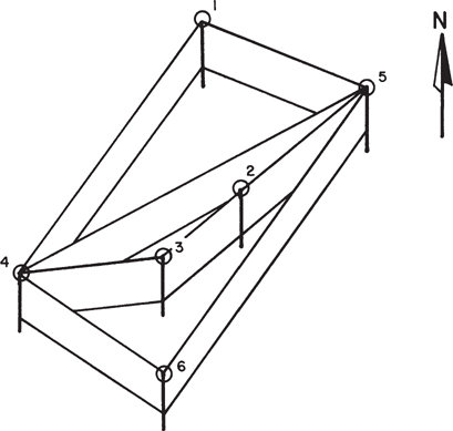
Figure 6-44 Typical fence diagram layout for the 9200-ft Sand. (From Boeckelman, unpublished. Published by permission of author.)
True length and slope measurements can be made.
More panels are available for study, providing more detailed and accurate analysis.
Because of the right-angle grid system, less data are obscured in this model as compared to other types of panel diagrams.
By measuring total net sand at each grid intersection and well location, it is possible to construct a more accurate net sand and net hydrocarbon isochore map.
The overall appearance of the model is more pleasing to the eye and is easier to understand and follow.
Figure 6-45 is another example of a completed 3D reservoir model. Compare this model with the fence diagram in Figure 6-38, which is constructed from the same well data. Notice how clearly the structure is represented in the 3D model (Fig. 6-45) compared to the fence diagram (Fig. 6-38). Also observe how much more data are presented with minimal obstruction in the 3D model. Finally, true length and slope can be measured on the model, which cannot be done with the fence diagram.
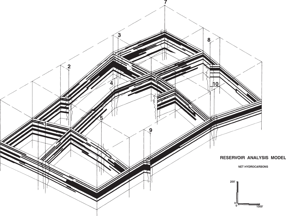
Figure 6-45 Compare this 3D RAM with the fence diagram in Figure 6-38, which was prepared from the same well data.
The use of 3D reservoir analysis models has become less common in recent years as the increased availability of computing power has made the construction of 3D geocellular models practical. These geocellular models not only capture the distribution of lithologies and reservoir and fluid properties in three dimensions, they also allow for the simulation of fluid flow within petroleum reservoirs.
Cross-Section Construction Using a Computer
The most significant advantage of building cross sections using a computer is that the geologist is actively viewing and interacting with the cross section during the interpretation process. In other words, rather than viewing the cross-section display as a final product, constructed for presentation purposes, cross-sectional views can be created at all phases of a geological interpretation to help guide the final result. For example, on the computer the geologist can set up cross-section displays that are designed primarily for correlation purposes and quickly re-datum and respace these cross sections to view the geometric implications of the evolving correlation interpretation. Cross sections can be constructed for many purposes, and with the computer, they can be created on-the-fly in a matter of seconds.
Correlation Cross Sections
During the log correlation phase of subsurface interpretation, the geologist can build cross-section displays, optimized for log correlation, that contain several dozen wells each. Figure 6-46 shows an eight-well correlation cross section through Pliocene sediments. Correlation sections can be set up to show any track of a series of electric logs. By limiting the view to just one track, several dozen closely spaced logs can be viewed on a computer screen at one time, and log picks can be rapidly correlated from the type well across these specialized cross-section panels. The track chosen for Figure 6-46 is the SP/GR track. Note the missing sections, due to faults, displayed in Wells No. 2, 3, 5, and 7 in the stratigraphically datumed cross section. Picking and “gapping” faults during the correlation phase of a study greatly facilitates sorting out the stratigraphy in complexly faulted regions (see section Computer-Based Log Correlation in Chapter 4). Deviated wells need to be corrected to a true vertical depth display utilizing the directional survey.
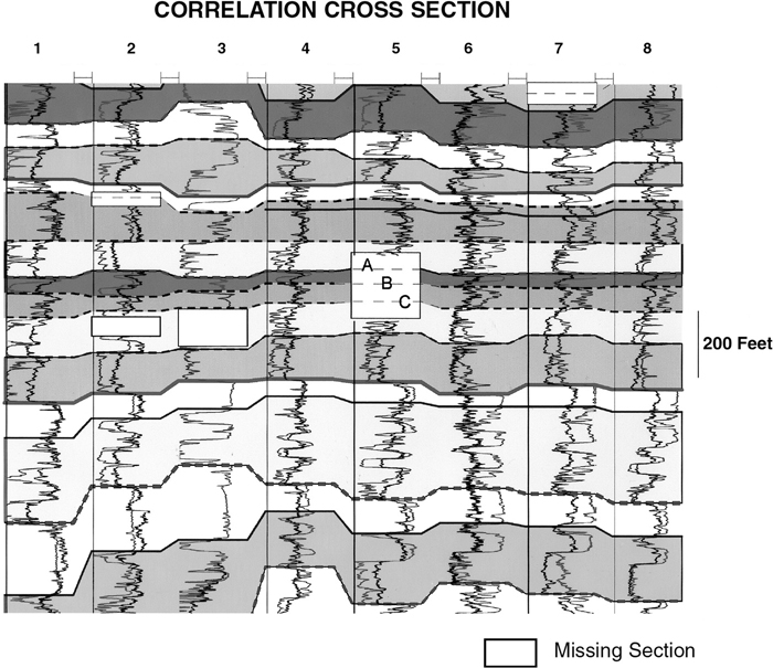
Figure 6-46 Eight-well, closely spaced correlation cross section set up to show the SP/GR track of a series of electric logs. The orientation of the section is constantly changing as all wells in the field study were included for correlation purposes. The missing section due to faulting is restored using a fault-gapping tool. Wells numbered 1 through 8 at the top of the section are all Mesa Petroleum-operated wells. (Published by permission of W. C. Ross and A2D Technologies.)
Stratigraphic Cross Sections
Stratigraphic cross sections are designed to reconstruct original depositional geometries prior to structural deformation. Computer-based cross-section software facilitates the construction of stratigraphic cross sections in a number of ways. The ability to quickly select any correlation and rehang the section on the selected datum allows the geologist to reconstruct, with the click of a button, depositional geometries for successive correlations. To properly reconstruct accurate stratigraphic geometries, wells can be spaced proportional to map distance (or projected to a line of section). For wells with deviated wellbores, the program used should be able to adjust the spacing of the wells to be proportional to map distance using the latitude and longitude positions along the chosen datum. Cross-section software should support the picking and termination of correlations, facies boundaries, and unconformities in the space between wells (Figs. 6-47 and 6-48). As wells are reordered or the section re-datumed from stratigraphic to structural views, the inter-well interpretation shifts appropriately (Fig. 6-47a and b).
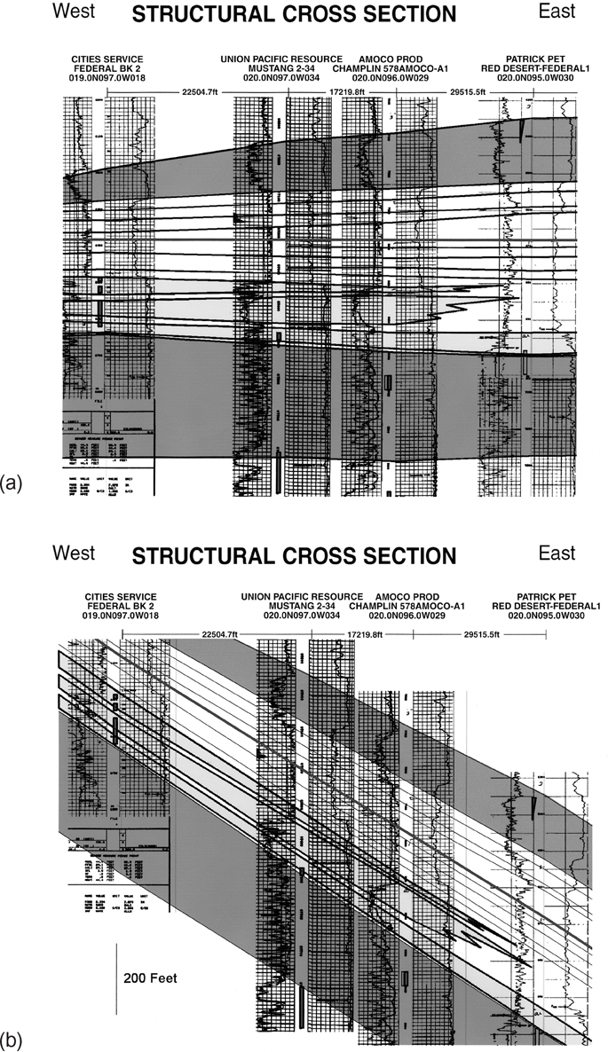
Figure 6-47 Stratigraphic (a) and structural (b) cross sections of Almond Formation and Lewis Formation stratigraphic relationships in the Green River Basin of Wyoming. Wells are spaced proportional to map distance. Facies changes and sandstone pinchouts, interpreted in the inter-well space in stratigraphic mode (a), are automatically repositioned properly in structural mode (b), and tops picked in the time-stratigraphic gap are used to determine and draw the position of onlap and erosional truncation terminations above and below the sequence boundary, respectively. (Published by permission of W. C. Ross and A2D Technologies.)
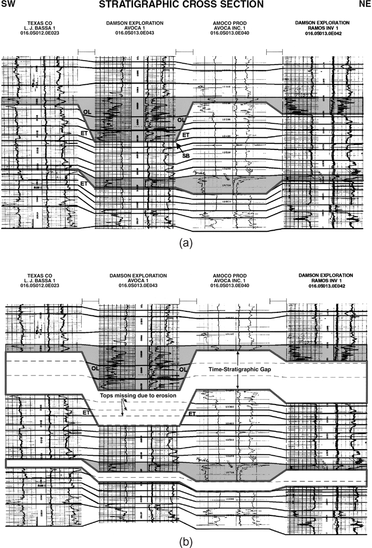
Figure 6-48 Stratigraphic cross sections of shallow marine and incised valley-fill sediments. (a) Shallow marine shelf facies are shown truncated by an incised-valley system. The base of the incised-valley system is a sequence boundary (SB). Erosional truncation (ET) of shelf strata below the sequence boundary and onlap (OL) of channel- fill strata above the unconformity are automatically positioned using the timeline geometries shown in (b). (b) The logs have been pulled apart, or “gapped,” at the sequence boundary to represent a missing section due to erosion and/or nondeposition. The intersection of the sequence boundary and tops picked in the time-stratigraphic gap are used to determine and draw the position of onlap and erosional truncation terminations above and below the sequence boundary, respectively. (Published by permission of W. C. Ross and A2D Technologies; and AAPG©1990, reprinted by permission of the AAPG whose permission is required for further use.)
Missing Section in Stratigraphic Cross Sections
Building stratigraphic cross sections can be enhanced by restoring those portions of the cross section that are missing due to erosion, nondeposition, or faulting. Unconformity/fault tools allow geologists to split or gap logs proportionally to reflect the amount of section lost due to erosion or faulting. An example of restoring a missing section due to channel erosion is illustrated in Figure 6-48a, where a siliciclastic package of marine shales and shelf sandstones is truncated by an incised valley system. Figure 6-48b shows the same system where the logs have been split, or gapped, at an unconformity (sequence) boundary. The gap space represents missing time due to erosion (in the valley) and nondeposition (in the interfluves). Correlations from the marine shale interfluve are extended into the missing section gap and represent an estimate of stratigraphic geometry prior to erosion. The ability to pick tops within these gaps allows geologists to hang cross sections on tops that have been cut out by erosion. Tops picked within the channel feature are extended into the interfluve space. When the gaps are closed, the software automatically determines the appropriate onlap and truncation geometries in the inter-well space, above and below the unconformity surface, respectively (Fig. 6-48a).
Structural Cross Sections
Structural cross sections are built by geologists as a complement to structure maps. Creating structural cross sections using a computer is simply a matter of selecting a structural datum and a well spacing proportional to map distance or projected to a line of section. These sections can be produced on-the-fly to check the validity of an evolving interpretation.
To include fault interpretations in a structural interpretation, the geologist first picks faults using an arbitrary, generic fault-naming scheme (Fig. 6-49). In this phase of interpretation, fault picks and missing section estimates can be interactively interpreted in “fault gap mode” by splitting the log and dragging down the fault gaps with a mouse-controlled fault tool (Fig. 4-33c and d in Computer-Based Log Correlation in Chapter 4). Once the generic fault locations in the wells are in place, the geologist can correlate or assign them with the same fault name (Fig. 6-50). These correlated faults each possess a missing section or vertical separation value interpreted by the geologist when the fault was first picked and after the gap was “pulled down” in gap mode. When the faults are correlated, these vertical separation values are interpolated from well to well to create an overall vertical separation fault function along the length of the fault. When the geologist instructs the software to create a structural cross section, the fault gaps are automatically closed and correlations intersecting the fault are automatically offset utilizing the vertical separation value at the fault-correlation intersection point (Fig. 6-51). The appropriate offset is determined using logic described in Chapter 4.

Figure 6-49 Stratigraphic cross section of Pliocene sediments. The missing section fault gaps show the results of fault identification through detailed correlation and vertical separation (VS) analysis. Estimates of a missing section (VS), due to faulting, have been performed at three locations and are shown within each missing section fault gap. Fault names are generic. As a result, no fault correlation is required at this stage of fault interpretation. Correlations A, B, and C are picked within the missing fault gap on the Mesa Petroleum OCS-G 03587 A-6 well. (Published by permission of W. C. Ross and A2D Technologies.)
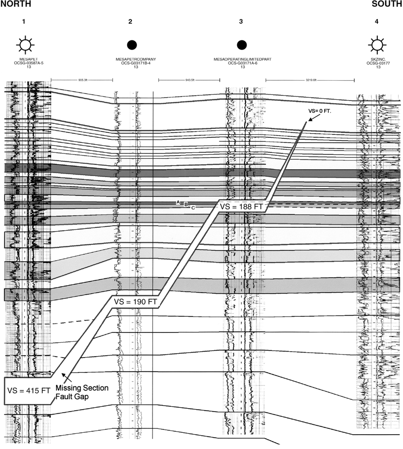
Figure 6-50 Stratigraphic cross section from Figure 6-49 showing fault geometry after geologist assigns a specific fault name to each generically named fault. (Published by permission of W. C. Ross and A2D Technologies.)

Figure 6-51 Structural cross section with fault and bed-offset geometry resulting from application of vertical-separation fault function to each fault-correlation intersection. Note upthrown and downthrown bed offsets of missing correlations A, B, and C to the left and right of cross-section Well No. 3. (Published by permission of W. C. Ross and A2D Technologies.)
In addition to being a significant time-saver in the construction of structural cross sections, the automated offsetting of correlations provides a powerful constraint on the attitude of beds in the inter-well area, including beds cut out by the fault (see offsets of correlations A, B, and C, which are missing at cross section Well No. 3 in Fig. 6-51).
The ability to interactively interpret fault location (depth) in a well and the amount of missing section (vertical separation), and then to pick markers within these missing-section gaps, provides the geologist with a powerful set of tools for subsurface interpretations in regions dominated by normal faults. Figure 6-52a and b show stratigraphic (with missing-section gaps) and structural versions of a cross section from the Wilcox of South Texas (Edwards 2001). The large faults have cut out hundreds of feet of section. Tops cut out by the faults have been picked within the missing-section gaps across the entire cross section. Missing-section stratigraphic cross sections are useful for removing structure and providing an undistorted view of the correlation framework (Fig. 6-52b).

Figure 6-52 (a) Structural cross section of faulted Wilcox strata in Zapata County, South Texas. Correlation offsets were calculated using interpolated vertical separation information interpreted at fault positions in wells. (b) Stratigraphic cross section with a missing section, due to faulting, shown as gaps. Note increasing size of missing-section fault gap in a down-dip direction for lowermost fault. This pattern depicts increasing amounts of vertical separation along the fault with depth. (Published by permission of W. C. Ross and A2D Technologies.)
One challenge with constructing cross sections on a computer is controlling the projection of wells into the section. Most if not all software systems project wells into a section using the normal-to-section projection method. As discussed earlier in this chapter, this projection method is not the preferred method in many cases. Some software systems allow the interpreter to manually project wells using alternative projection systems such as plunge projection, structural strike projection, fault-strike projection, and so on. Using these alternative projections, which are preferred in many instances, requires a geologist to manually control how wells are projected, assuming that the software package being used allows this manual control, as the software does not know the plunge or strike of a structure. Having to project wells by hand obviates some, but not all, of the advantages of constructing cross sections on the computer.
Fault-Seal Analysis
The evaluation of potential hydrocarbon seal along a fault surface can be critical to exploration and development prospects and to reservoir evaluation. Some aspects of this analysis that are typically considered are (1) juxtaposition of rock units, which we can classify as a structural or geometric aspect; (2) lithologic characteristics of the fault zone such as shale smear, fault gouge, and the rock types that are juxtaposed along the fault; (3) pressure differentials across the fault zone; and (4) possible vertical conductivity of the fault. Given the context of this book, we address only techniques by which you can determine juxtaposition of rock units across a fault. This determination provides the structural basis for a complete fault-seal analysis. We describe in detail a manual structural method and summarize a computer-based evaluation of juxtaposition.
Studies of faulted reservoirs in the Gulf Coast Tertiary (Smith 1980) indicate that sands that are juxtaposed against themselves across a fault are very unlikely to be sealed at that fault. Sands that are juxtaposed across a fault against a sealing lithology are very likely to be sealed at the fault. Sands that are juxtaposed across a fault against a sand of a different age are sometimes sealed at the fault. Analysis of the sealing potential of a fault generally begins with a study of juxtaposition of beds across the fault.
Analysis of juxtaposition typically involves a depiction of the fault surface showing the traces of stratigraphic units on the footwall and hanging wall. The interpreted fault surface itself may be used, or a horizontal projection of the traces can be made from the interpreted fault surface onto a vertical plane parallel to the strike of the fault. Either method portrays the juxtaposition of units across the fault. Allan (1980, 1989) is generally credited with introducing the technique into the oil industry, although the first widely available description of Allan’s technique was by Downey (1984). Rippon (1985) described the construction of fault plane sections for use in the coal mining industry in the United Kingdom. Bouvier et al. (1989) apply a technique known as fault slicing (seismic sections parallel to the trace of a fault) to examine the seal characteristics of faults in offshore Nigeria. Fault surface sections are used extensively to evaluate sealing characteristics of faults (e.g., Broussard and Lock 1995; Yielding et al. 1997).
Fault Surface Sections Constructed by Hand
Fault surface sections, variously referred to as fault plane sections, fault profile sections, juxtaposition diagrams, or Allan sections, are simply cross sections with the fault surface as the plane of section. Allan (1980, 1989) proposed this idea to show the juxtaposition of permeable units along the length of a fault. A standard cross section shows the juxtaposition of units only at a single place along the fault. The objective is to build a cross section that shows where reservoir rocks might communicate across the fault and use this information to evaluate the trapping potential of the fault. Plotting permeable intervals (based on well logs and seismic data) for adjacent fault blocks on the same cross section shows the separation and juxtaposition of the permeable units across the fault. For convenience, the fault surface section typically represents a vertical plane onto which the rock units are projected from the fault surface.
Structure maps on the top and base of permeable units are the basic data needed (for simplicity, we refer herein to such units as “sands”). The method requires structure maps with the fault traces accurately mapped, as described in Chapter 8, because the fault traces show the location and depth of the intersection of the sand and the fault surface. To build a fault surface section, you could just overlay cross-section paper on a top-of-sand structure map and trace the fault traces, both upthrown and downthrown, from the map onto the cross section. This would be the intersection of the top of sand with the fault surface along the length of the fault. Then overlay the same cross-section paper on the base-of-sand map in exactly the same position and copy the fault traces from the map. Any overlap of a top of sand with a base of sand would show juxtaposition of sand across the fault. The difficulty with this method is that the vertical scale of the cross section is the same as the horizontal scale. At a map scale of 1 in. = 1000 ft, a 100-ft sand would appear only about one-tenth of an inch thick on the cross section. This would make interpretation difficult. Many cross sections use some vertical exaggeration, and this is generally necessary for fault surface sections. As discussed earlier in this chapter, this distorts the true geometry of the units, but the purpose of a fault surface section is only to show juxtaposition of units, and such distortions do not interfere with this purpose. Also, the curvature of the fault surface introduces other distortions in the cross section, but they do not adversely affect fault surface sections either. Finally, the method itself introduces some thickness distortion as structure maps are maps of surfaces projected into a horizontal plane; thus the top and base of sand on the cross section are not in the plane of the fault.
In practice, the vertical scale of a fault surface section is in depth, so the top and base of sand are projected into a vertical plane that is more or less parallel to the strike of the fault surface. Broussard and Lock (1995) referred to this vertical plane as the Allan plane. Figure 6-53 shows a profile of this vertical plane on a standard cross section, with the projection of the sands onto it from the intersections of the top and base of sand with the fault surface. No juxtaposition exists in this case. Figure 6-54 demonstrates, with the same structure, a pitfall of using sand thickness to determine the base-of-sand intersection with the fault surface. Note that the apparent sand thickness as projected onto the Allan plane is smaller than the TVT and the stratigraphic thickness of the sand. If, as a shortcut, the TVT thickness were used to determine base of sand within dipping beds at the fault, then it could indicate juxtaposition where there is none (Fig. 6-54). Also, if apparent throw is compared to TVT of the sand and found to be less than the TVT, a false juxtaposition could be inferred. To avoid these pitfalls, always use both the top and base of sand to portray the sand face correctly on the fault surface section.
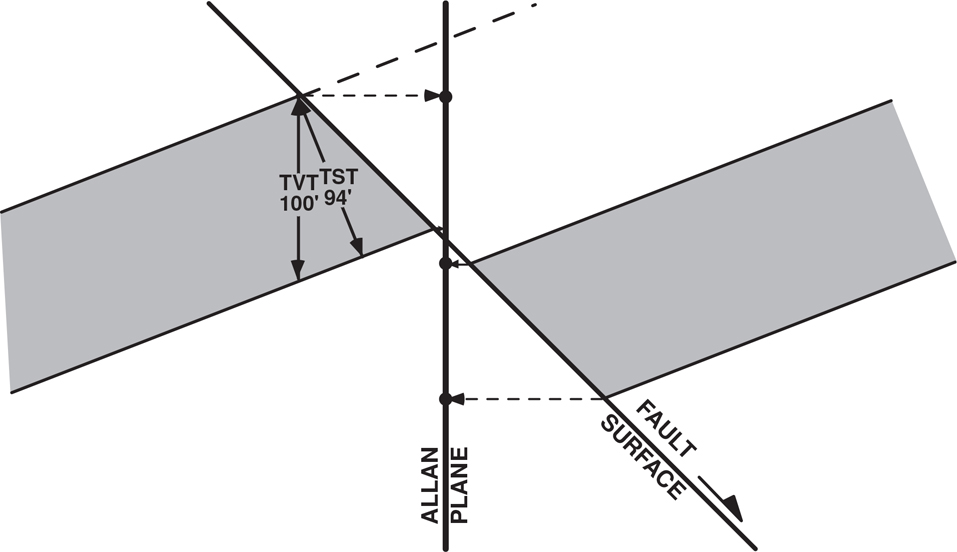
Figure 6-53 A cross section of a faulted sand bed showing the correct projection of the sand from the fault surface to the vertical Allan plane. (After Broussard and Lock 1995. Published by permission of the Gulf Coast Association of Geological Societies.)
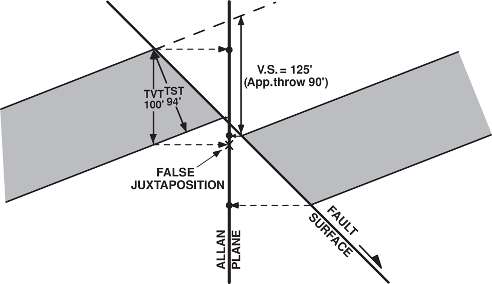
Figure 6-54 A cross section of a faulted sand bed showing an incorrect projection of the sand from the fault surface to the Allan plane. False juxtaposition can be indicated by using bed thickness for the base of sand or by comparing apparent throw to bed thickness. (After Broussard and Lock 1995. Published by permission of the Gulf Coast Association of Geological Societies.)
Figure 6-55 illustrates the process of constructing a fault surface section or Allan section from structure maps. The steps are similar to building a finished illustration (show) cross section, as described elsewhere in this chapter, except the line of section is the fault surface projected into a vertical plane. To illustrate the method, we use one sand offset by a fault and evaluate the juxtaposition of the sand.
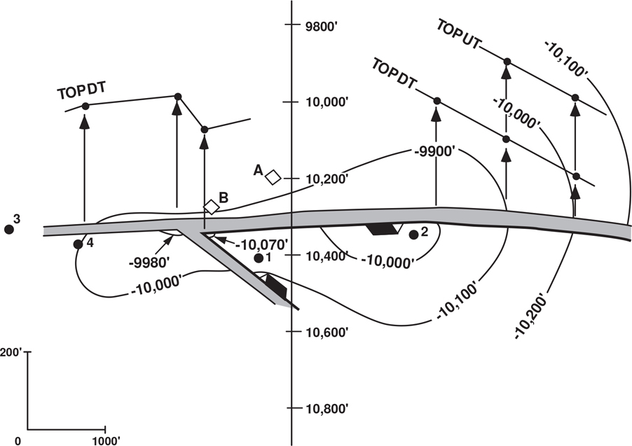
Figure 6-55 A fault surface section is constructed by overlaying depth-scaled cross-section paper on a structure map of the top of sand, with the depth scale perpendicular to the fault trace. The depths of the upthrown and downthrown traces for the top of sand are plotted on the cross section. Although not illustrated here, the traces of the base of sand are then plotted from a base-of-sand map. Wells 1, 2, 3, and 4 and Platforms A and B are used to register the cross section in the same place on both maps. (After Broussard and Lock 1995. Published by permission of the Gulf Coast Association of Geological Societies.)
For the fault surface section, select a convenient depth scale that covers the range of depths along the fault for the top-of-sand and base-of-sand maps. Overlay the cross-section paper on the top-of-sand structure map with the vertical depth scale more or less perpendicular to the fault trace on the map. Mark some registration points, such as well locations, so you can locate the cross section paper in exactly the same place from map to map. In the example, the vertical exaggeration is 5:1.
Determine the depth of the fault trace for the top of sand in the upthrown block and plot it on the cross-section paper. For example, from the structure map, find where the −10,000-ft contour intersects with the fault trace upthrown and project parallel to the depth scale to the −10,000-ft depth on the cross section and mark a point. Continue along the upthrown fault trace, plotting the depths onto the cross section (interpolating the depth where necessary). Then connect the points with a line to plot the top of the sand at the fault.
Plot the depth of the fault trace for the top of sand in the downthrown block in the same manner. At intersections with other faults, estimate the depth in the corners of the intersection, plot these points on the cross section, and connect them with a straight line. This is the top of sand as it would be on the subject fault surface at the intersecting fault, according to the structure map.
Next, although we do not illustrate it, you would repeat the process for a base-of-sand map by plotting the upthrown and downthrown traces of the base of sand. The same registration points used for the top-of-sand map will allow you to locate the cross-section paper in exactly the same place on the base of sand map.
Finally, as shown in Figure 6-56, color or shade any overlap or juxtaposition of the sand, or sands if you are plotting more than one. Minor variations in contouring between the top-and base-of-sand maps usually should not affect the juxtaposition interpretation, but they should be evaluated for their significance to the accuracy of the maps.

Figure 6-56 A fault surface section of a thick sand with the area shaded gray where the sand is juxtaposed to itself. (After Broussard and Lock 1995. Published by permission of the Gulf Coast Association of Geological Societies.)
Commonly, the fault displacement is sufficient to juxtapose different sands. For this situation, choose a depth interval suitable to the sand(s) of interest in one fault block and then determine which sand(s) in the other block fall within that depth range. Follow the steps above, using the structure maps of the top and base of each sand within its respective fault block.
Plotting the depth of the fault traces for the tops and bases of permeable intervals on cross-section paper gives a graphical display of the faces of the intervals against the fault surface that can easily be interpreted for juxtaposition of the intervals. Accurate fault surface maps and top- and base-of-sand maps are necessary for a valid fault surface section.
Computer-Based Fault-Seal Analysis
Modern visualization software provides a means of viewing a fault surface that was interpreted within a data volume on the basis of seismic and well data. An interpreter can examine the fault surface in isometric view, usually looking toward the footwall and in a direction perpendicular to the fault surface. The presentation considerably enhances the interpreter’s ability to evaluate whether the fault surface is reasonable, based on aspects such as fault geometry and displacement patterns, which can be plotted on the surface (Needham et al. 1996). Furthermore, juxtaposition of stratigraphic units can be readily examined if horizon data, such as tops and bases of permeable units, at the footwall and hanging wall are plotted as traces on the fault surface. The displayed data are derived directly from the interpreted data volume.
Application of 3D Modeling and Visualization Techniques.
The computer-based method in which the fault surface is modeled in three dimensions eliminates the projection errors that are common in the traditional method for constructing fault plane sections. More importantly, the 3D representation portrays the fault surface in a true structural context within the prospect itself and in relation to other faults.
A 3D fault surface is constructed by modeling the fault segments picked on vertical (in-line or cross-line) or horizontal (time slice) sections, either on a grid or by using triangulation algorithms (Fig. 6-57). The surface can then be viewed in perspective to provide an assessment of the plausibility of the interpreted fault geometry. Horizon terminations at their respective fault segments are used to plot footwall and hanging wall horizon traces on the perspective view of the fault surface, allowing the interpreter to observe in detail how reservoir layers are juxtaposed by the fault. The horizon separation information can also be used to calculate displacement-related values (throw, heave, vertical separation), which may be gridded or triangulated over the entire fault surface in order to produce displacement maps on the 3D representation of the fault surface. Fault displacement can also be used to calculate other attributes, such as fault-seal potential, which can be posted on the perspective view of the fault surface.
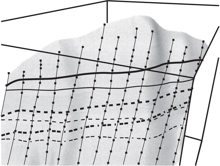
Figure 6-57 Footwall (thick lines and dashes) and hanging wall (thin lines and dashes) projected onto a normal fault surface. Vertical lines with nodes represent the fault surface intersection with the vertical seismic lines. (Published by permission of Badley Earth Sciences.)
Fault-Seal Potential.
Fault seal can be due to juxtaposition of reservoir rock against nonreservoir rock or to fault-zone material of high entry-pressure (e.g., clay smear in the fault zone) (Yielding et al. 1997). Both seal types are dependent on fault displacement and the nature and distribution of lithologies in the wall rocks (Figs. 6-58 and 6-59). The 3D representation of the entire fault surface allows fault-seal attributes to be mapped onto the fault surface. A detailed description of the various methods to predict fault-seal potential, with examples using fault surface sections, can be found in Yielding et al. 1997 and Yielding et al. 2010.
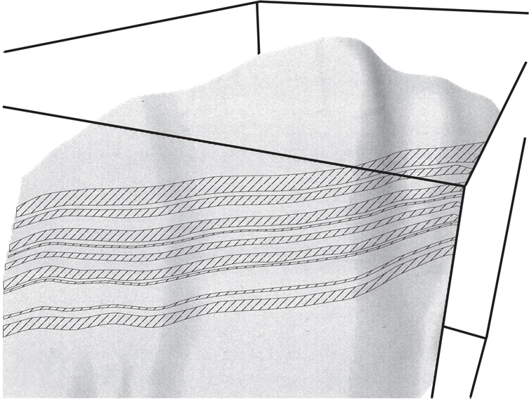
Figure 6-58 Fault surface showing sands in the footwall of a normal fault. (Published by permission of Badley Earth Sciences.)
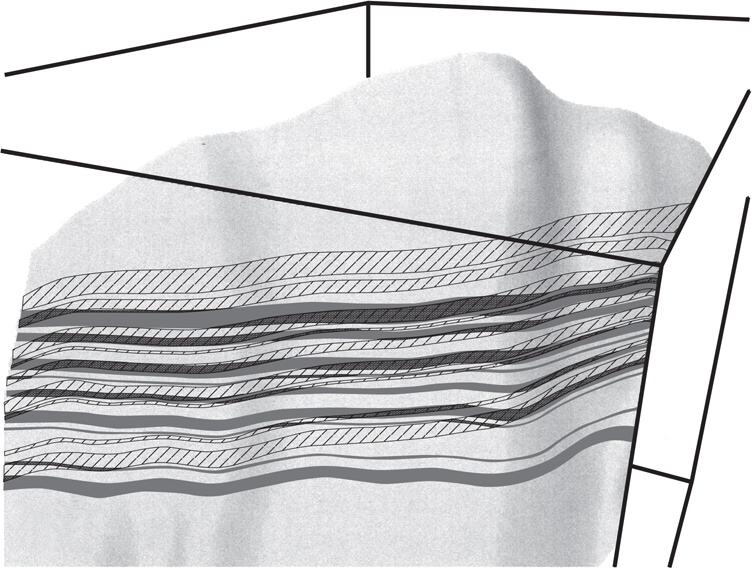
Figure 6-59 Fault surface showing sands in the footwall (hachure pattern) and the hanging wall (solid pattern), and sand juxtaposition where the two patterns overlap. (Published by permission of Badley Earth Sciences.)
Identification of juxtaposition of reservoir units across the fault surface (Fig. 6-59) uses horizons mapped from seismic and well data and a detailed reservoir stratigraphy defined by isochores. Probable seals due to juxtaposition (sands on one side of the fault in contact with impermeable lithologies, commonly shales) can be clearly identified along the fault surface (Fig. 6-59). Similarly, overlaps of juxtaposed reservoir units (e.g., sand against sand) can be explicitly displayed (Fig. 6-60). Remember that the accuracy of horizon interpretation is paramount to the precision of this juxtaposition display and analysis and therefore to the ultimate depiction of the reservoirs.

Figure 6-60 Fault surface showing the overlaps of juxtaposed reservoir units. (Published by permission of Badley Earth Sciences.)
Once the overlap of permeable units is determined, as in Figure 6-60, an analysis can be made of whether a given contact is likely to support a pressure difference due to lithologic attributes (e.g., gouge ratio, shale smear). Refer to Yielding et al. (1997, 2010) for a detailed discussion.
Conclusions
Fault surface sections, whether depicted as vertical sections parallel to the strike of the fault or as 3D representations of the fault surface, offer a unique view within the 3D data volume. The sections provide data about the fault, the quality of the interpretation, and especially the fault’s potential for sealing hydrocarbons. The routine construction and analysis of fault surface sections should be adopted as a crucial part of the workflow in exploration and production projects.
Chronostratigraphic Sections
We describe here a chronostratigraphic cross section used by stratigraphers and sequence stratigraphers. Chronostratigraphic sections are plotted with the y-axis in geological time and the x-axis in distance (Fig. 6-61). Chronostratigraphic sections are sometimes called Wheeler diagrams (Sloss 1984) after Harry Wheeler, who proposed this type of plot (Wheeler 1958). Chronostratigraphic sections are not used in mapping, but they are extremely useful in exploration because they illustrate the history of a basin. Also important is that the sections can show the distribution of facies across the basin at various times. Source, seal, and reservoir units can be highlighted. Chronostratigraphic sections are usually accompanied with a map that illustrates the line of section. Several chronostratigraphic sections are shown in Figures 6-62 and 6-63.
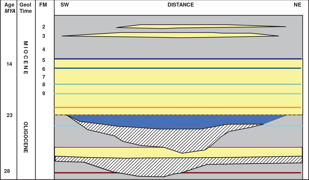
Figure 6-61 Generic chronostratigraphic section illustrating the change in lithology with time and along the line of the section. Hachured intervals equal times of erosion and nondeposition. (Modified from Shoup 2017. Used with permission of R. Shoup.)

Figure 6-62 A chronostratigraphic section from the Nam Con Son Basin in Southeast Asia. This chronostratigraphic section illustrates the geological history of a basin. Various additional pieces of information, such as seafloor magnetic reversals, sea level curve, biostratigraphy, formation names, and orogenic events, are plotted on the vertical axis along with geological time. Lithology is based on stratigraphy seen in individual wells across the basin. (Modified from Swiecicki and Maynard, 2009; used with permission of Dr. Tony Swiecicki.) Register on the InformIT site (see preface) to view the full-sized color figure.

Figure 6-63 A chronographic section across the Dampier Sub-Basin, offshore northwest Australia. This chronographic section shows the specific wells going into the section. (From Norvick 2001. Published with permission from M. S. Norvick.)