Chapter 8
Time intelligence calculations
Almost any data model includes some sort of calculation related to dates. DAX offers several functions to simplify these calculations, which are useful if the underlying data model follows certain specific requirements. On the other hand, if the model contains peculiarities in the handling of time that would prevent the use of standard time intelligence functions, then writing custom calculations is always an option.
In this chapter, you learn how to implement common date-related calculations such as year-to-date, year-over-year, and other calculations over time including nonadditive and semi-additive measures. You learn both how to use specific time intelligence functions and how to rely on custom DAX code for nonstandard calendars and week-based calculations.
Introducing time intelligence
Typically, a data model contains a date table. In fact, when slicing data by year and month, it is preferable to use the columns of a table specifically designed to slice dates. Extracting the date parts from a single column of type Date or DateTime in calculated columns is a less desirable approach.
There are several reasons for this choice. By using a date table, the model becomes easier to browse, and you can use specific DAX functions that perform time intelligence calculations. In fact, in order to work properly, most of the time intelligence functions in DAX require a separate date table.
If a model contains multiple dates, like the order date and the delivery date, then one can either create multiple relationships with a single date table or duplicate the date table. The resulting models are different, and so are the calculations. Later in this chapter, we will discuss these two alternatives in more detail.
In any case, one should always create at least one date table whenever there are one or more date columns in the data. Power BI and Power Pivot for Excel offer embedded features to automatically create tables or columns to manage dates in the model, whereas Analysis Services has no specific feature for the handling of time intelligence. However, the implementation of these features does not always follow the best practice of keeping a single date table in the data model. Also, because these features come with several restrictions, it is usually better to use your own date table. The next sections expand on this last statement.
Automatic Date/Time in Power BI
Power BI has a feature called Auto Date/Time, which can be configured through the options in the Data Load section (see Figure 8-1).

When the setting is enabled—it is by default—Power BI automatically creates a date table for each Date or DateTime column in the model. We will call it a “date column” from here on. This makes it possible to slice each date by year, quarter, month, and day. These automatically created tables are hidden to the user and cannot be modified. Connecting to the Power BI Desktop file with DAX Studio makes them visible to any developers curious about their structure.
The Auto Date/Time feature comes with two major drawbacks:
Power BI Desktop generates one table per date column. This creates an unnecessarily high number of date tables in the model, unrelated to one another. Building a simple report presenting the amount ordered and the amount sold in the same matrix proves to be a real challenge.
The tables are hidden and cannot be modified by the developer. Consequently, if one needs to add a column for the weekday, they cannot.
Building a proper date table for complete freedom is a skill that you learn in the next few pages, and it only requires a few lines of DAX code. Forcing your model to follow bad practices in data modeling just to save a couple of minutes when building the model for the first time is definitely a bad choice.
Automatic date columns in Power Pivot for Excel
Power Pivot for Excel also has a feature to handle the automatic creation of data structures, making it easier to browse dates. However, it uses a different technique that is even worse than that of Power BI. In fact, when one uses a date column in a pivot table, Power Pivot automatically creates a set of calculated columns in the same table that contains the date column. Thus, it creates one calculated column for the year, one for the month name, one for the quarter, and one for the month number—required for sorting. In total, it adds four columns to your table.
As a bad practice, it shares all the bad features of Power BI and it adds a new one. In fact, if there are multiple date columns in a single table, then the number of these calculated columns will start to increase. There is no way to use the same set of columns to slice different dates, as is the case with Power BI. Finally, if the date column is in a table with millions of rows—as is often the case—these calculated columns increase the file size and the memory footprint of the model.
This feature can be disabled in the Excel options, as you can see in Figure 8-2.
Date table template in Power Pivot for Excel
Excel offers another feature that works much better than the previous feature. Indeed, since 2017 there is an option in Power Pivot for Excel to create a date table, which can be activated through the Power Pivot window, as shown in Figure 8-3.

In Power Pivot, clicking on New creates a new table in the model with a set of calculated columns that include year, month, and weekday. It is up to the developer to create the correct set of relationships in the model. Also, if needed, one has the option to modify the names and the formulas of the calculated columns, as well as adding new ones.
There is also the option of saving the current table as a new template, which will be used in the future for newly created date tables. Overall, this technique works well. The table generated by Power Pivot is a regular date table that fulfills all the requirements of a good date table. This, in conjunction with the fact that Power Pivot for Excel does not support calculated tables, makes the feature useful.
Building a date table
As you have learned, the first step for handling date calculations in DAX is to create a date table. Because of its relevance, one should pay attention to some details when creating the date table. In this section, we provide the best practices regarding the creation of a date table. There are two different aspects to consider: a technical aspect and a data modeling aspect.
From a technical point of view, the date table must follow these guidelines:
The date table contains all dates included in the period to analyze. For example, if the minimum and maximum dates contained in Sales are July 3, 2016, and July 27, 2019, respectively, the range of dates of the table is between January 1, 2016, and December 31, 2019. In other words, the date table needs to contain all the days for all the years containing sales data. There can be no gaps in the sequence of dates. All dates need to be present, regardless of whether there are transactions or not on each date.
The date table contains one column of DateTime type, with unique values. The Date data type is a better choice because it guarantees that the time part is empty. If the DateTime column also contains a time part, then all the times of the day need to be identical throughout the table.
It is not necessary that the relationship between Sales and the date table be based on the Date-Time column. One can use an integer to relate the two tables, yet the DateTime column needs to be present.
The table should be marked as a Date table. Though this is not a strictly mandatory step, it greatly helps in writing correct code. We will cover the details of this feature later in this chapter.
![]() Important
Important
It is common for newbies to create a huge date table with many more years than needed. That is a mistake. For example, one might create a date table with two hundred years ranging from 1900 to 2100, just in case. Technically the date table works fine, but there will be serious performance issues whenever it is used in calculations. Using a table with only the relevant years is a best practice.
From the technical point of view, a table containing a single date column with all the required dates is enough. Nevertheless, a user typically wants to analyze information slicing by year, month, quarter, weekday, and many other attributes. Consequently, a good date table should include a rich set of columns that—although not used by the engine—greatly improve the user experience.
If you are loading the date table from an existing data source, then it is likely that all the columns describing a date are already present in the source date table. If necessary, additional columns can be created as calculated columns or by changing the source query. Performing simple calculations in the data source is preferable whenever possible—reducing the use of calculated columns to when they are strictly required. Alternatively, you can create the date table by using a DAX calculated table. We describe the calculated table technique along with the CALENDAR and CALENDARAUTO functions in the next sections.
![]() Note
Note
The term “Date” is a reserved keyword in DAX; it corresponds to the DATE function. Therefore, you should embed the Date name in quotes when referring to the table name, despite the fact that there are no spaces or special characters in that name. You might prefer using Dates instead of Date as the name of the table to avoid this requirement. However, it is better to be consistent in table names, so if you use the singular form for all the other table names, it is better to keep it singular for the date table too.
Using CALENDAR and CALENDARAUTO
If you do not have a date table in your data source, you can create the date table by using either CALENDAR or CALENDARAUTO. These functions return a table of one column, of DateTime data type. CALENDAR requires you to provide the upper and lower boundaries of the set of dates. CALENDAR-AUTO scans all the date columns across the entire data model, finds the minimum and maximum years referenced, and finally generates the set of dates between these years.
For example, a simple calendar table containing all the dates in the Sales table can be created using the following code:
Date =
CALENDAR (
    DATE ( YEAR ( MIN ( Sales[Order Date] ) ), 1, 1 ),
    DATE ( YEAR ( MAX ( Sales[Order Date] ) ), 12, 31 )
)
In order to force all dates from the first of January up to the end of December, the code only extracts the minimum and maximum years, forcing day and month to be the first and last of the year. A similar result can be obtained by using the simpler CALENDARAUTO:
Date = CALENDARAUTO ( )
CALENDARAUTO scans all the date columns, except for calculated columns. For example, if one uses CALENDARAUTO to create a Date table in a model that contains sales between 2007 and 2011 and has an AvailableForSaleDate column in the Product table starting in 2004, the result is the set of all the days between January 1, 2004, and December 31, 2011. However, if the data model contains other date columns, they affect the date range considered by CALENDARAUTO. Storing dates that are not useful to slice and dice is very common. For example, if among the many dates a model also contains the customers’ birthdates, then the result of CALENDARAUTO starts from the oldest year of birth of any customer. This produces a large date table, which in turn negatively affects performance.
CALENDARAUTO accepts an optional parameter that represents the final month number of a fiscal year. If provided, CALENDARAUTO generates dates from the first day of the following month to the last day of the month indicated as an argument. This is useful when you have a fiscal year that ends in a month other than December. For example, the following expression generates a Date table for fiscal years starting on July 1 and ending on June 30:
Date = CALENDARAUTO ( 6 )
CALENDARAUTO is slightly easier to use than CALENDAR because it automatically determines the boundaries of the set of dates. However, it might extend this set by considering unwanted columns. One can obtain the best of both worlds by restricting the result of CALENDARAUTO to only the desired set of dates, as follows:
Date =
VAR MinYear = YEAR ( MIN ( Sales[Order Date] ) )
VAR MaxYear = YEAR ( MAX ( Sales[Order Date] ) )
RETURN
FILTER (
    CALENDARAUTO ( ),
    YEAR ( [Date] ) >= MinYear &&
    YEAR ( [Date] ) <= MaxYear
)
The resulting table only contains the useful dates. Finding the first and last day of the year is not that important because CALENDARAUTO handles this internally.
Once the developer has obtained the correct list of dates, they still must create additional columns using DAX expressions. Following is a list of commonly used expressions for this scope, with an example of their results in Figure 8-4:
Date =
VAR MinYear = YEAR ( MIN ( Sales[Order Date] ) )
VAR MaxYear = YEAR ( MAX ( Sales[Order Date] ) )
RETURN
ADDCOLUMNS (
     FILTER (
         CALENDARAUTO ( ),
         YEAR ( [Date] ) >= MinYear &&
         YEAR ( [Date] ) <= MaxYear
     ),
     "Year", YEAR ( [Date] ),
     "Quarter Number", INT ( FORMAT ( [Date], "q" ) ),
     "Quarter", "Q" & INT ( FORMAT ( [Date], "q" ) ),
     "Month Number", MONTH ( [Date] ),
     "Month", FORMAT ( [Date], "mmmm" ),
     "Week Day Number", WEEKDAY ( [Date] ),
     "Week Day", FORMAT ( [Date], "dddd" ),
     "Year Month Number", YEAR ( [Date] ) * 100 + MONTH ( [Date] ),
     "Year Month", FORMAT ( [Date], "mmmm" ) & " " & YEAR ( [Date] ),
     "Year Quarter Number", YEAR ( [Date] ) * 100 + INT ( FORMAT ( [Date], "q" ) ),
     "Year Quarter", "Q" & FORMAT ( [Date], "q" ) & "-" & YEAR ( [Date] )
)
Instead of using a single ADDCOLUMNS function, one could achieve the same result by creating several calculated columns through the user interface. The main advantage of using ADDCOLUMNS is the ability to reuse the same DAX expression to create a date table in other projects.
Working with multiple dates
When there are multiple date columns in the model, you should consider two design options: creating multiple relationships to the same date table or creating multiple date tables. Choosing between the two options is an important decision because it affects the required DAX code and also the kind of analysis that is possible later on.
Consider a Sales table with the following three dates for every sales transaction:
Order Date: the date when an order was received.
Due Date: the date when the order is expected to be delivered.
Delivery Date: the actual delivery date.
The developer can relate the three dates to the same date table, knowing that only one of the three relationships can be active. Or, they can create three date tables in order to be able to slice by any of the three freely. Besides, it is likely that other tables contain other dates. For example, a Purchase table might contain other dates about the purchase process, a Budget table contains other dates in turn, and so on. In the end, every data model typically contains several dates, and one needs to understand the best way to handle all these dates.
In the next sections, we show two design options to handle this scenario and how this affects the DAX code.
Handling multiple relationships to the Date table
One can create multiple relationships between two tables. Nevertheless, only one relationship can be active. The other relationships need to be kept inactive. Inactive relationships can be activated in CALCULATE through the USERELATIONSHIP modifier introduced in Chapter 5, “Understanding CALCULATE and CALCULATETABLE.”
For example, consider the data model shown in Figure 8-5. There are two different relationships between Sales and Date, but only one can be active. In the example, the active relationship is the one between Sales[Order Date] and Date[Date].
![The model shows two relationships between Sales and Date. Only the one between Sales[Order Date] and Date[Date] is active.](http://images-20200215.ebookreading.net/5/4/4/9780134865867/9780134865867__definitive-guide-to__9780134865867__graphics__08fig05.jpg)
You can create two measures for the sales amount based on a different relationship to the Date table:
Ordered Amount :=
SUMX ( Sales, Sales[Net Price] * Sales[Quantity] )

Delivered Amount :=
CALCULATE (
    SUMX ( Sales, Sales[Net Price] * Sales[Quantity] ),
    USERELATIONSHIP ( Sales[Delivery Date], 'Date'[Date] )
)
The first measure, Ordered Amount, uses the active relationship between Sales and Date, based on Sales[Order Date]. The second measure, Delivered Amount, executes the same DAX expression using the relationship based on Sales[Delivery Date]. USERELATIONSHIP changes the active relationship between Sales and Date in the filter context defined by CALCULATE. You can see in Figure 8-6 an example of a report using these measures.

Using multiple relationships with a single date table increases the number of measures in the data model. Generally, one only defines the measures that are meaningful with certain dates. If you do not want to handle a large number of measures, or if you want complete freedom of using any measure with any date, then you might consider implementing calculation groups as explained in the following chapter.
Handling multiple date tables
Instead of duplicating every measure, an alternative approach is to create different date tables—one for each date in the model—so that every measure aggregates data according to the date selected in the report. From a maintenance point of view, this might seem like a better solution because it lowers the number of measures, and it allows for the selecting of sales that intersect between two months, but it produces a model that is harder to use. For example, one can easily produce a report with the total number of orders received in January and delivered in February of the same year—but it is harder to show in the same chart the amounts ordered and delivered by month.
This approach is also known as the role-playing dimension approach. The date table is a dimension that you duplicate once for each relationship—that is, once for each of its roles. These two options (using inactive relationships and duplicating the date table) are complementary to each other.
To create a Delivery Date table and an Order Date table, you add the same table twice in the data model. You must at least modify the table name when doing so. You can see in Figure 8-7 the data model containing two different date tables related to Sales.

![]() Important
Important
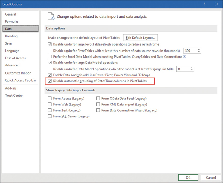
You must physically duplicate the Date table. Therefore, it is a best practice to create different views in the data source, one for each role dimension, so that each date table has different column names and different content. For example, instead of having the same Year column in all the date tables, it is better if you use Order Year and Delivery Year. Navigating the report will be easier this way. This is also visible in Figure 8-7. Furthermore, it is also a good practice to change the content of columns; for instance, by placing a prefix for the year depending on the role of the date. As an example, one might use the CY prefix for the content of the Order Year column and the DY prefix for the content of the Delivery Year column.
Figure 8-8 shows an example of a matrix using multiple date tables. Such a report cannot be created using multiple relationships with a single Date table. You can see that renaming column names and content is important to produce a readable result. In order to avoid confusion between order and delivery dates, we used CY as a prefix for order years and DY as a prefix for delivery years.
Using multiple date tables, the same measure displays different results depending on the columns used to slice and dice. However, it would be wrong to choose multiple date tables just to reduce the number of measures because this makes it impossible to create a report with the same measures grouped by two dates. For example, consider a single line chart showing Sales Amount by Order Date and Delivery Date. One needs a single Date table in the date axis of the chart, and this would be extremely complex to achieve with the multiple date tables pattern.
If your first priority is to reduce the number of measures in a model, enabling the user to browse any measure by any date, you should consider using the calculation groups described in Chapter 9, “Calculation groups,” implementing a single date table in the model. The main scenario where multiple date tables are useful is to intersect the same measure by different dates in the same visualization, as demonstrated in Figure 8-8. In most other scenarios, a single date table with multiple relationships is a better choice.
Understanding basic time intelligence calculations
In the previous sections you learned how to correctly build a date table. The date table is useful to perform any time intelligence calculation. DAX provides several time intelligence functions that simplify such calculations. It is easy to use those functions and build useful calculations. Nevertheless, it is all too easy to start using those functions without a good understanding of their inner details. For educational purposes, in this section we demonstrate how to author any time intelligence calculation by using standard DAX functions such as CALCULATE, CALCULATETABLE, FILTER, and VALUES. Then, later in this chapter, you learn how the time intelligence functions in DAX help you shorten your code and make it more readable.
There are multiple reasons why we decided to use this approach. The main driver is that, when it comes to time intelligence, there are many different calculations that cannot be expressed by simply using standard DAX functions. At some point in your DAX career, you will need to author a measure more complex than a simple year-to-date (YTD) discovering that DAX has no predefined functions for your requirements. If you learned to code time intelligence the hard way, this will not be a problem. You will roll up your sleeves and write the correct filter function without the help of DAX predefined calculations. If, on the other hand, you simply leverage standard DAX functions, then complex time intelligence will be problematic to solve.
Here is a general explanation of how time intelligence calculations work. Consider a simple measure; its evaluation happens in the current filter context:
Sales Amount :=
SUMX ( Sales, Sales[Net Price] * Sales[Quantity] )
Because Sales has a relationship with Date, the current selection on Date determines the filter over Sales. To perform the calculation over Sales in a different period, the programmer needs to modify the existing filter on Date. For example, to compute a YTD when the filter context is filtering February 2007, they would need to change the filter context to include January and February 2007, before performing the iteration over Sales.
A solution for this is to use a filter argument in a CALCULATE function, which returns the year-to-date up to February 2007:
Sales Amount Jan-Feb 2007 :=
CALCULATE (
SUMX ( Sales, Sales[Net Price] * Sales[Quantity] ),
FILTER (
ALL ( 'Date' ),
AND (
'Date'[Date] >= DATE ( 2007, 1, 1 ),
'Date'[Date] <= DATE ( 2007, 2, 28 )
)
)
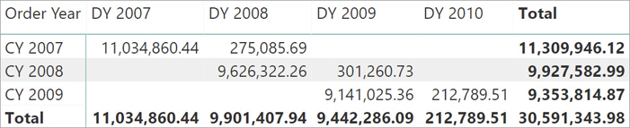
)The result is visible in Figure 8-9.
The FILTER function used as a filter argument of CALCULATE returns a set of dates that replaces the selection of the Date table. In other words, even though the original filter context coming from the rows of the matrix filters an individual month, the measure computes the value on a different set of dates.
Obviously, a measure that returns the sum of two months is not useful. Nevertheless, once you understand the basic mechanism, you can use it to write a different calculation that computes the year-to-date such as the following code:
Sales Amount YTD :=
VAR LastVisibleDate = MAX ( 'Date'[Date] )
VAR CurrentYear = YEAR ( LastVisibleDate )
VAR SetOfDatesYtd =
    FILTER (
        ALL ( 'Date' ),
        AND (
            'Date'[Date] <= LastVisibleDate,
            YEAR ( 'Date'[Date] ) = CurrentYear
        )
    )
VAR Result =
    CALCULATE (
        SUMX ( Sales, Sales[Net Price]  * Sales[Quantity] ),
        SetOfDatesYtd
    )
RETURN
    Result
Though this code is a bit more complex than the previous code, the pattern is the same. In fact, this measure first retrieves in LastVisibleDate the last date selected in the current filter context. Once the date is known, it extracts its year and saves it in the CurrentYear variable. The third variable SetOfDatesYtd contains all the dates in the current year, before the end of the current period. This set is used to replace the filter context on the date to compute the year-to-date, as you can see in Figure 8-10.

As explained earlier, one could write a time intelligence calculation without using time intelligence functions. The important concept here is that time intelligence calculations are not different from any other calculation involving filter context manipulation. Because the measure needs to aggregate values from a different set of dates, the calculation happens in two steps. First, it determines the new filter for the date. Second, it applies the new filter context before computing the actual measure. All time intelligence calculations behave the same way. Once you understand the basic concept, then time intelligence calculations will have no secrets for you.
Before moving further with more time intelligence calculations, it is important to describe a special behavior of DAX when handling relationships that are based on a date. Look at this slightly different formulation of the same code, where instead of filtering the entire date table, we only filter the Date[Date] column:
Sales Amount YTD :=
VAR LastVisibleDate = MAX ( 'Date'[Date] )
VAR CurrentYear = YEAR ( LastVisibleDate )
VAR SetOfDatesYtd =
    FILTER (
        ALL ( 'Date'[Date] ),
        AND (
            'Date'[Date] <= LastVisibleDate,
            YEAR ( 'Date'[Date] ) = CurrentYear
        )
    )
VAR Result
    CALCULATE (
        SUMX ( Sales, Sales[Net Price]  * Sales[Quantity] ),
        SetOfDatesYtd
    )
RETURN
    Result
If someone uses this measure in a report instead of the previous measure, they will see no changes. In fact, the two versions of this measure compute exactly the same value, but they should not. Let us examine in detail one specific cell—for example, April 2007.
The filter context of the cell is Year 2007, Month April. As a consequence, LastVisibleDate contains the 30th of April 2007, whereas CurrentYear contains 2007. Then because of its formulation, SetOfDatesYtd contains all the dates between January 1, 2007, up to April 30, 2007. In other words, in the cell of April 2007, the code executed is equivalent to this:
CALCULATE (
    CALCULATE (
        [Sales Amount],
        AND (                                       -- This filter is equivalent
            'Date'[Date] >= DATE ( 2007, 1, 1),     -- to the result of the FILTER
            'Date'[Date] <= DATE ( 2007, 04, 30 )   -- function
        )
    ),
    'Date'[Year] = 2007,                            -- These are coming from the rows
    'Date'[Month] = "April"                         -- of the matrix in April 2007
)
If you recall what you learned about filter contexts and the CALCULATE behavior, you should verify that this code should not compute a correct year-to-date. Indeed, the inner CALCULATE filter argument returns a table containing the Date[Date] column. As such, it should overwrite any existing filter on Date[Date], keeping other filters on other columns untouched. Because the outer CALCULATE applies a filter to Date[Year] and to Date[Month], the final filter context where [Sales Amount] is computed should only contain April 2007. Nevertheless, the measure actually computes a correct result including the other months since January 2007.
The reason is a special behavior of DAX when the relationship between two tables is based on a date column, as it happens for the relationship with Date in the demo model we are using here. Whenever a filter is applied to a column of type Date or DateTime that is used in a relationship between two tables, DAX automatically adds an ALL to the entire Date table as an additional filter argument to CALCULATE. In other words, the previous code should read this way:
CALCULATE (
    CALCULATE (
        [Sales Amount],
        AND (                                       -- This filter is equivalent
            'Date'[Date] >= DATE ( 2007, 1, 1),     -- to the result of the FILTER
            'Date'[Date] <= DATE ( 2007, 04, 30 )   -- function
        ),
        ALL ( 'Date' )    -- This is automatically added by the engine
    ),
    'Date'[Year] = 2007,                            -- These are coming from the rows
    'Date'[Month] = "April"                         -- of the matrix in April 2007
)
Every time a filter is applied on the column that defines a one-to-many relationship with another table, and the column has a Date or DateTime data type, DAX automatically propagates the filter to the other table and overrides any other filter on other columns of the same lookup table.
The reason for this behavior is to make time intelligence calculations work more simply in the case where the relationship between the date table and the sales table is based on a date column. In the next section, we describe the behavior of the Mark as Date Table feature, which introduces a similar behavior for relationships not based on a date column.
Using Mark as Date Table
Applying a filter on the date column of a calendar table works fine if the date column also defines the relationship. However, one might have a relationship based on another column. Many existing date tables use an integer column—typically in the format YYYYMMDD—to create the relationship with other tables.
In order to demonstrate the behavior, we created the DateKey column in both the Date and Sales tables. We then linked the two using the DateKey column instead of the date column. The resulting model is visible in Figure 8-11.

Using the same code that worked in previous examples to compute the YTD in Figure 8-11 would result in an incorrect calculation. You see this in Figure 8-12.

As you can see, now the report shows the same value for Sales Amount and for Sales Amount YTD. Indeed, since the relationship is no longer based on a DateTime column, DAX does not add the automatic ALL function to the date table. As such, the filter with the date is intersecting with the previous filter, vanishing the effect of the measure.
In such cases there are two possible solutions: one is to manually add ALL to all the time intelligence calculations. This solution is somewhat cumbersome because it requires the DAX coder to always remember to add ALL to all of the calculations. The other possible solution is much more convenient: mark the Date table as a date table.
If the date table is marked as such, then DAX will automatically add ALL to the table even if the relationship was not based on a date column. Be mindful that once the table is marked as a date table, the automatic ALL on the table is always added whenever one modifies the filter context on the date column. There are scenarios where this effect is undesirable, and in such cases, one would need to write complex code to build the correct filter. We cover this later in this chapter.
Introducing basic time intelligence functions
Now that you have learned the basic mechanism that runs time intelligence calculations, it is time to simplify the code. Indeed, if DAX developers had to write complex FILTER expressions every time they need a simple year-to-date calculation, their life would be troublesome.
To simplify the authoring of time intelligence calculations, DAX offers a rich set of functions that automatically perform the same filtering we wrote manually in the previous examples. For example, this is the version of Sales Amount YTD measure we wrote earlier:
Sales Amount YTD :=
VAR LastVisibleDate = MAX ( 'Date'[Date] )
VAR CurrentYear = YEAR ( LastVisibleDate )
VAR SetOfDatesYTD =
    FILTER (
        ALL ( 'Date'[Date] ),
        AND (
            'Date'[Date] <= LastVisibleDate,
            YEAR ( 'Date'[Date] ) = CurrentYear
        )
    )
VAR Result =
    CALCULATE (
        SUMX ( Sales, Sales[Net Price]  * Sales[Quantity] ),
        SetOfDatesYTD
    )
RETURN
    Result
The same behavior can be expressed by a much simpler code using the DATESYTD function:
Sales Amount YTD :=
CALCULATE (
    SUMX ( Sales, Sales[Net Price]  * Sales[Quantity] ),
    DATESYTD ( 'Date'[Date] )
)
Be mindful that DATESYTD does exactly what the more complex code performs. The gain is neither in performance nor in behavior of the code. However, because it is so much easier to write, you see that learning the many time intelligence functions in DAX is worth your time.
Simple calculations like year-to-date, quarter-to-date, month-to-date, or the comparison of sales in the current year versus the previous year can be authored with simpler code as they all rely on basic time intelligence functions. More complex calculations can oftentimes be expressed by mixing standard time intelligence functions. The only scenario where the developer will really need to author complex code is when they need nonstandard calendars, like a weekly calendar, or for complex time intelligence calculations when the standard functions will not meet the requirements.
![]() Note
Note
All time intelligence functions in DAX apply a filter condition on the date column of a Date table. You can find some examples of how to write these calculations in DAX later in this book and a complete list of all the time intelligence features rewritten in plain DAX at http://www.daxpatterns.com/time-patterns/.
In the next sections, we introduce the basic time intelligence calculations authored with the standard time intelligence functions in DAX. Later in this chapter, we will cover more advanced calculations.
Using year-to-date, quarter-to-date, and month-to-date
The calculations of year-to-date (YTD), quarter-to-date (QTD), and month-to-date (MTD) are all very similar. Month-to-date is meaningful only when you are looking at data at the day level, whereas year-to-date and quarter-to-date calculations are often used to look at data at the month level.
You can calculate the year-to-date value of sales for each month by modifying the filter context on dates for a range that starts on January 1 and ends on the month corresponding to the calculated cell. You see this in the following DAX formula:
Sales Amount YTD :=
CALCULATE (
[Sales Amount],
DATESYTD ( 'Date'[Date] )
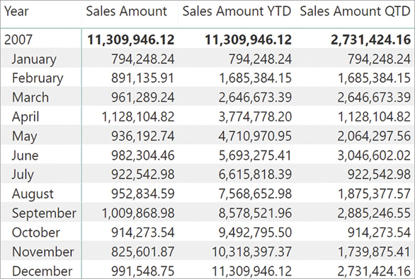
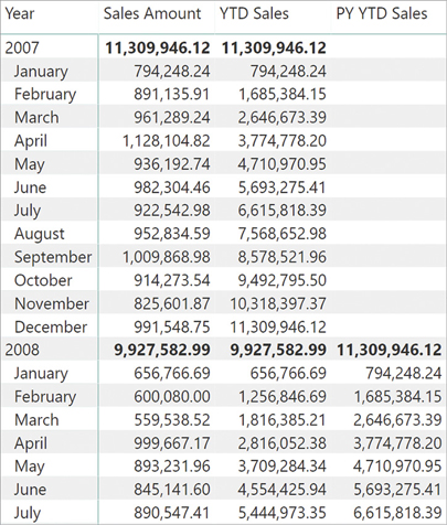
)DATESYTD is a function that returns a table with all the dates from the beginning of the year until the last date included in the current filter context. This table is used as a filter argument in CALCULATE to set the new filter for the Sales Amount calculation. Similar to DATESYTD, there are another two functions that return the month-to-date (DATESMTD) and quarter-to-date (DATESQTD) sets. For example, you can see measures based on DATESYTD and DATESQTD in Figure 8-13.
This approach requires the use of CALCULATE. DAX also offers a set of functions to simplify the syntax of to-date calculations: TOTALYTD, TOTALQTD, and TOTALMTD. In the following code, you can see the year-to-date calculation expressed using TOTALYTD:
YTD Sales :=
TOTALYTD (
    [Sales Amount],
    'Date'[Date]
)
The syntax is somewhat different, as TOTALYTD requires the expression to aggregate as its first parameter and the date column as its second parameter. Nevertheless, the behavior is identical to the original measure. The name TOTALYTD hides the underlying CALCULATE function, which is a good reason to limit its use. In fact, whenever CALCULATE is present in the code, making it evident is always a good practice—for example, for the context transition it implies.
Similar to year-to-date, you can also define quarter-to-date and month-to-date with built-in functions, as in these measures:
QTD Sales := TOTALQTD ( [Sales Amount], 'Date'[Date] )
QTD Sales := CALCULATE ( [Sales Amount], DATESQTD ( 'Date'[Date] ) )
MTD Sales := TOTALMTD ( [Sales Amount], 'Date'[Date] )
MTD Sales := CALCULATE ( [Sales Amount], DATESMTD ( 'Date'[Date] ) )
Calculating a year-to-date measure over a fiscal year that does not end on December 31 requires an optional third parameter that specifies the end day of the fiscal year. For example, both the following measures calculate the fiscal year-to-date for Sales:
Fiscal YTD Sales := TOTALYTD ( [Sales Amount], 'Date'[Date], "06-30" )
Fiscal YTD Sales := CALCULATE ( [Sales Amount], DATESYTD ( 'Date'Date], "06-30" ) )
The last parameter corresponds to June 30—that is, the end of the fiscal year. There are several time intelligence functions that have a last, optional year-end date parameter for this purpose: STARTOFYEAR, ENDOFYEAR, PREVIOUSYEAR, NEXTYEAR, DATESYTD, TOTALYTD, OPENINGBALANCEYEAR, and CLOSINGBALANCEYEAR.
![]() Important
Important
Depending on the culture settings, you might have to use the day number first. You can also consider using a string with the format YYYY-MM-DD to avoid any ambiguity caused by culture settings; in that case, the year does not matter for the purpose of determining the last day of the year to use for year-to-date calculation:
Fiscal   YTD Sales := TOTALYTD ( [Sales Amount], 'Date'[Date], "30-06"  )
Fiscal  YTD Sales := CALCULATE ( [Sales Amount], DATESYTD ( 'Date'[Date], "30-06" ) )
Fiscal YTD Sales := CALCULATE ( [Sales Amount], DATESYTD ('Date'[Date],"2018-06-30" ) )
However, consider that as of June 2018 there is a bug in case the fiscal year starts in March and ends in February. More details and a workaround are described later in the “Advanced time intelligence” section of this chapter.
Computing time periods from prior periods
Several calculations are required to get a value from the same period in the prior year (PY). This can be useful for making comparisons of trends during a time period this year to the same time period last year. In that case SAMEPERIODLASTYEAR comes in handy:
PY Sales := CALCULATE ( [Sales Amount], SAMEPERIODLASTYEAR ( 'Date'[Date] ) )
SAMEPERIODLASTYEAR returns a set of dates shifted one year back in time. SAMEPERIODLASTYEAR is a specialized version of the more generic DATEADD function, which accepts the number and type of period to shift. The types of periods supported are YEAR, QUARTER, MONTH, and DAY. For example, you can define the same PY Sales measure using this equivalent expression, which uses DATEADD to shift the current filter context one year back in time:
PY Sales := CALCULATE( [Sales Amount], DATEADD ( 'Date'[Date], -1, YEAR ) )
DATEADD is more powerful than SAMEPERIODLASTYEAR because, in a similar way, DATEADD can compute the value from a previous quarter (PQ), month (PM), or day (PD):
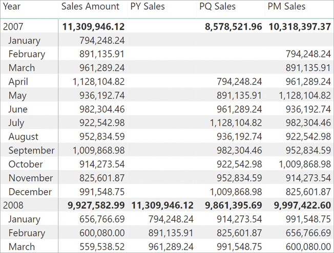
PQ Sales := CALCULATE ( [Sales Amount], DATEADD ( 'Date'[Date], -1, QUARTER ) )
PM Sales := CALCULATE ( [Sales Amount], DATEADD ( 'Date'[Date], -1, MONTH ) )
PD Sales := CALCULATE ( [Sales Amount], DATEADD ( 'Date'[Date], -1, DAY ) )
In Figure 8-14 you can see the result of some of these measures.
Another useful function is PARALLELPERIOD, which is similar to DATEADD, but returns the full period specified in the third parameter instead of the partial period returned by DATEADD. Thus, although a single month is selected in the current filter context, the following measure using PARALLEPERIOD calculates the amount of sales for the whole previous year:
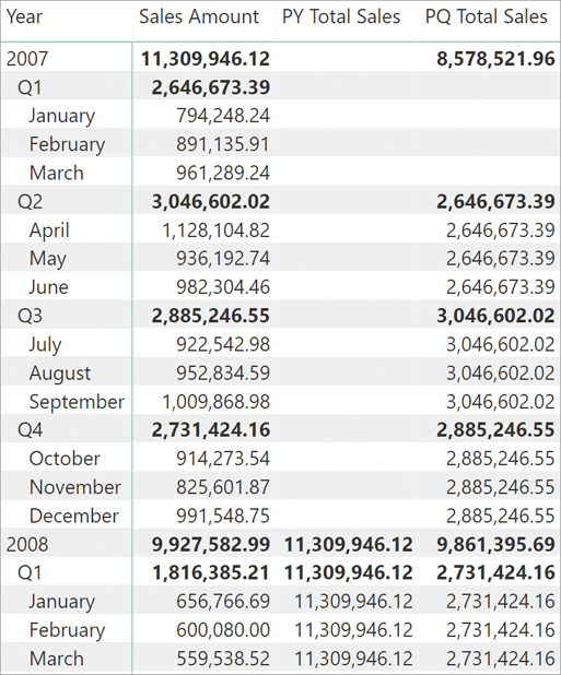
PY Total Sales :=
CALCULATE ( [Sales Amount], PARALLELPERIOD ( 'Date'[Date], -1, YEAR ) )
In a similar way, using different parameters, one can obtain different periods:
PQ Total Sales :=
CALCULATE ( [Sales Amount], PARALLELPERIOD ( 'Date'[Date], -1, QUARTER ) )
In Figure 8-15 you can see PARALLELPERIOD used to compute the previous year and quarter.
There are functions similar but not identical to PARALLELPERIOD, which are PREVIOUSYEAR, PREVIOUSQUARTER, PREVIOUSMONTH, PREVIOUSDAY, NEXTYEAR, NEXTQUARTER, NEXTMONTH, and NEXTDAY. These functions behave like PARALLELPERIOD when the selection has a single element selected corresponding to the function name—year, quarter, month, and day. If multiple periods are selected, then PARALLELPERIOD returns a shifted result of all of them. On the other hand, the specific functions (year, quarter, month, and day, respectively) return a single element that is contiguous to the selected period regardless of length. For example, the following code returns March, April, and May 2008 in case the second quarter of 2008 (April, May, and June) is selected:
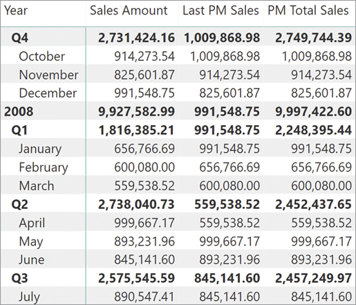
PM Total Sales :=
CALCULATE ( [Sales Amount], PARALLELPERIOD ( 'Date'[Date], -1, MONTH ) )
Conversely, the following code only returns March 2008 in case the second quarter of 2008 (April, May, and June) is selected.
Last PM Sales :=
CALCULATE ( [Sales Amount], PREVIOUSMONTH( 'Date'[Date] ) )
The difference between the two measures is visible in Figure 8-16. The Last PM Sales measure returns the value of December 2007 for both 2008 and Q1 2008, whereas PM Total Sales always returns the value for the number of months of the selection—three for a quarter and twelve for a year. This occurs even though the initial selection is shifted back one month.
Mixing time intelligence functions
One useful feature of time intelligence functions is the capability of composing more complex formulas by using time intelligence functions together. The first parameter of most time intelligence functions is the date column in the date table. However, this is just syntax sugar for the complete syntax. In fact, the full syntax of time intelligence functions requires a table as its first parameter, as you can see in the following two equivalent versions of the same measure. When used, the date column referenced is translated into a table with the unique values active in the filter context after a context transition, if a row context exists:
PY Sales :=
CALCULATE (
    [Sales Amount],
    DATESYTD ( 'Date'[Date] )
)

-- is equivalent to

PY Sales :=
CALCULATE (
    [Sales Amount],
    DATESYTD ( CALCULATETABLE ( DISTINCT ( 'Date'[Date] ) ) )
)
Time intelligence functions accept a table as their first parameter, and they act as time shifters. These functions take the content of the table, and they shift it back and forth over time by any number of years, quarters, months, or days. Because time intelligence functions accept a table, any table expression can be used in place of the table—including another time intelligence function. This makes it possible to combine multiple time intelligence functions, by cascading their results one into the other.
For example, the following code compares the year-to-date with the corresponding value in the previous year. It does so by combining SAMEPERIODLASTYEAR and DATESYTD. It is interesting to note that exchanging the order of the function calls does not change the result:
PY YTD Sales :=
CALCULATE (
    [Sales Amount],
    SAMEPERIODLASTYEAR ( DATESYTD ( 'Date'[Date] ) )
)

-- is equivalent to

PY YTD Sales :=
CALCULATE (
    [Sales Amount],
    DATESYTD ( SAMEPERIODLASTYEAR ( 'Date'[Date] ) )
)
It is also possible to use CALCULATE to move the current filter context to a different time period and then invoke a function that, in turn, analyzes the filter context and moves it to a different time period. The following two definitions of PY YTD Sales are equivalent to the previous two; YTD Sales and PY Sales measures are defined earlier in this chapter:
PY YTD Sales :=
CALCULATE (
    [YTD Sales],
    SAMEPERIODLASTYEAR ( 'Date'[Date] )
)
-- is equivalent to

PY YTD Sales :=
CALCULATE (
    [PY Sales],
    DATESYTD ( 'Date'[Date] )
)
You can see the results of PY YTD Sales in Figure 8-17. The values of YTD Sales are reported for PY YTD Sales, shifted one year ahead.
All the examples seen in this section can operate at the year, quarter, month, and day levels, but not at the week level. Time intelligence functions are not available for week-based calculations because there are too many variations of years/quarters/months based on weeks. For this reason, you must implement DAX expressions to handle week-based calculations. You can find more details and an example of this approach in the “Working with custom calendars” section, later in this chapter.
Computing a difference over previous periods
A common operation is calculating the difference between a measure and its value in the prior year. You can express that difference as an absolute value or as a percentage. You have already seen how to obtain the value for the prior year with the PY Sales measure:
PY Sales := CALCULATE ( [Sales Amount], SAMEPERIODLASTYEAR ( 'Date'[Date] ) )
For Sales Amount, the absolute difference over the previous year (year-over-year or YOY) is a simple subtraction. However, you need to add a failsafe if you want to only show the difference when both values are available. In that case, variables are important to avoid calculating the same measure twice. You can define a YOY Sales measure with the following expression:
YOY Sales :=
VAR CySales = [Sales Amount]
VAR PySales = [PY Sales]
VAR YoySales =
    IF (
        NOT ISBLANK ( CySales ) && NOT ISBLANK ( PySales ),
        CySales - PySales
    )
RETURN
    YoySales
The equivalent calculation for comparing the year-to-date measure with a corresponding value in the prior year is a simple subtraction of two measures, YTD Sales and PY YTD Sales. You learned those in the previous section:
YTD Sales := TOTALYTD ( [Sales Amount], 'Date'[Date] )

PY YTD Sales :=
CALCULATE (
    [Sales Amount],
    DATESYTD ( SAMEPERIODLASTYEAR ( 'Date'[Date] ) )
)

YOY YTD Sales :=
VAR CyYtdSales = [YTD Sales]
VAR PyYtdSales = [PY YTD Sales]
VAR YoyYtdSales =
    IF (
        NOT ISBLANK ( CyYtdSales ) && NOT ISBLANK ( PyYtdSales ),
        CyYtdSales - PyYtdSales
    )
RETURN
    YoyYtdSales
Often, the year-over-year difference is better expressed as a percentage in a report. You can define this calculation by dividing YOY Sales by PY Sales; this way, the difference uses the previous year value as a reference for the percentage difference (100 percent corresponds to a value that is doubled in one year). In the following expressions that define the YOY Sales% measure, the DIVIDE function avoids a divide-by-zero error if there is no corresponding data in the prior year:
YOY Sales% := DIVIDE ( [YOY Sales], [PY Sales] )
A similar calculation displays the percentage difference of a year-over-year comparison for the year-to-date aggregation. The following definition of YOY YTD Sales% implements this calculation:
YOY YTD Sales% := DIVIDE ( [YOY YTD Sales], [PY YTD Sales] )
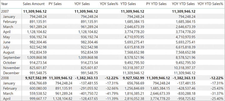
In Figure 8-18, you can see the results of these measures in a report.
Computing a moving annual total
Another common calculation that eliminates seasonal changes in sales is the moving annual total (MAT), which considers the sales aggregation over the past 12 months. You learned a technique to compute a moving average in Chapter 7, “Working with iterators and with CALCULATE.” Here we want to describe a formula to compute a similar average by using time intelligence functions.
For example, summing the range of dates from April 2007 to March 2008 calculates the value of MAT Sales for March 2008. The easiest approach is to use the DATESINPERIOD function. DATESINPERIOD returns all the dates included within a period that can be a number of years, quarters, months, or days.
MAT Sales :=
CALCULATE (                           -- Compute the sales amount in a new filter
    [Sales Amount],                   -- context modified by the next argument.
    DATESINPERIOD (                   -- Returns a table containing
        'Date'[Date],                 -- Date[Date] values,
        MAX ( 'Date'[Date] ),         -- starting from the last visible date
       -1,                            -- and going back 1
       YEAR                           -- year.
    )
)
Using DATESINPERIOD is usually the best option for the moving annual total calculation. For educational purposes, it is useful to see other techniques to obtain the same filter. Consider this alternative MAT Sales definition, which calculates the moving annual total for sales:
MAT Sales :=
CALCULATE (
    [Sales Amount],
    DATESBETWEEN (
        'Date'[Date],
        NEXTDAY ( SAMEPERIODLASTYEAR ( LASTDATE ( 'Date'[Date] ) ) ),
        LASTDATE ( 'Date'[Date] )
    )
)
The implementation of this measure requires some attention. The formula uses the DATESBETWEEN function, which returns the dates from a column included between two specified dates. Because DATESBETWEEN works at the day level, even if the report is querying data at the month level, the code must calculate the first day and the last day of the required interval. A way to obtain the last day is by using the LASTDATE function. LASTDATE is like MAX, but instead of returning a value, it returns a table. Being a table, it can be used as a parameter to other time intelligence functions. Starting from that date, the first day of the interval is computed by requesting the following day (by calling NEXTDAY) of the corresponding date one year before (by using SAMEPERIODLASTYEAR).
One problem with moving annual totals is that they compute the aggregated value—the sum. Dividing this value by the number of months included in the period averages it over the time frame. This gives you a moving annual average (MAA):
MAA Sales :=
CALCULATE (
    DIVIDE ( [Sales Amount], DISTINCTCOUNT ( 'Date'[Year Month] ) ),
    DATESINPERIOD (
        'Date'[Date],
        MAX ( 'Date'[Date] ),
       -1,
       YEAR
    )
)
As you have seen, using time intelligence functions results in powerful measures. In Figure 8-19, you can see a report that includes the moving annual total and average calculations.

Using the right call order for nested time intelligence functions
When nesting time intelligence functions, it is important to pay attention to the order used in the nesting. In the previous example, we used the following DAX expression to retrieve the first day of the moving annual total:
NEXTDAY ( SAMEPERIODLASTYEAR ( LASTDATE ( 'Date'[Date] ) ) )
You would obtain the same behavior by inverting the call order between NEXTDAY and SAMEPERIODLASTYEAR, as in the following code:
SAMEPERIODLASTYEAR ( NEXTDAY ( LASTDATE ( 'Date'[Date] ) ) )
The result is almost always the same, but this order of evaluation presents a risk of producing incorrect results at the end of the period. In fact, authoring the MAT code using this order would result in this version, which is wrong:
MAT Sales Wrong :=
CALCULATE (
    [Sales Amount],
    DATESBETWEEN (
        'Date'[Date],
        SAMEPERIODLASTYEAR ( NEXTDAY ( LASTDATE ( 'Date'[Date] ) ) ),
        LASTDATE ( 'Date'[Date] )
    )
)
This version of the formula computes the wrong result at the upper boundary of the date range. You can see this happening in a report like the one in Figure 8-20.
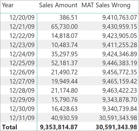
The measure computes the correct value up to December 30, 2009. Then, on December 31 the result is surprisingly high. The reason for this is that on December 31, 2009 NEXTDAY should return a table containing January 1, 2010. Unfortunately, the date table does not contain a row with January 1, 2010; thus, NEXTDAY cannot build its result. Consequently, not being able to return a valid result, NEXTDAY returns an empty table. A similar behavior happens with the following function: SAMEPERIODLASTYEAR. It receives an empty table, and as the result, it returns an empty table too. Because DATESBETWEEN requires a scalar value, the empty result of SAMEPERIODLASTYEAR is considered as a blank value. Blank—as a DateTime value—equals zero, which is December 30, 1899. Thus, on December 31, 2009, DATESBETWEEN returns the whole set of dates in the Date table; indeed, the blank as a starting date defines no boundaries for the initial date, and this results in an incorrect result.
The solution is straightforward. It simply involves using the correct order of evaluation. If SAMEPERIODLASTYEAR is the first function called, then on December 31, 2009, it will return a valid date, which is December 31, 2008. Then, NEXTDAY returns January 1, 2009, that this time does exist in the Date table.
In general, all time intelligence functions return sets of existing dates. If a date does not belong to the Date table, then these functions return an empty table that corresponds to a blank scalar value. In some scenarios this behavior might produce unexpected results, as explained in this section. For the specific example of the moving annual total, using DATESINPERIOD is simpler and safer, but this concept is important in case time intelligence functions are combined for other custom calculations.
Understanding semi-additive calculations
The techniques you have learned so far to aggregate values from different time periods work fine with regular additive measures. An additive measure is a calculation that aggregates values using a regular sum when sliced by any attribute. As an example, think about the sales amount. The sales amount of all the customers is the sum of the sales amount of each individual customer. At the same time, the sales amount of a full year is the sum of the sales amount of all the days in the year. There is nothing special about additive measures; they are intuitive and easy to use and to understand.
However, not all calculations are additive. Some measures are non-additive. An example would be a distinct count of the gender of the customers. For each individual customer, the result is 1. But when computed over a set of customers including different genders, the result will never be greater than the number of genders (three in case of Contoso—blank, M, and F). Thus, the result over a set of customers, dates, or any other column cannot be computed by summing individual values. Nonadditive measures are frequent in reports, oftentimes associated with distinct counts calculations. Nonadditive measures are more difficult to use and to understand than regular additive measures. However, regarding additivity, they are not the hardest ones. Indeed, there is a third kind of measure, the semi-additive measure, that proves to be challenging.
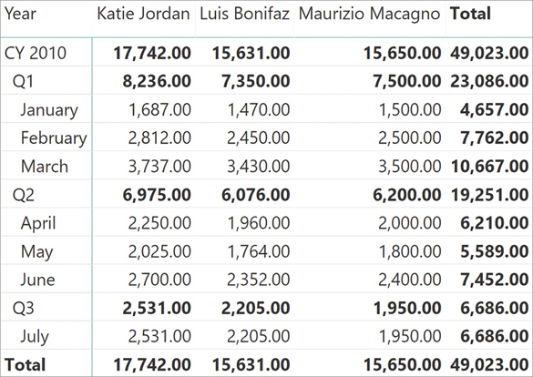
A semi-additive measure uses one kind of aggregation (typically a sum) when sliced by certain columns and a different kind of aggregation (usually the last date) when sliced by other columns. A great example is the balance of a bank account. The balance of all the customers is the sum of each individual balance. However, the balance over a full year is not the sum of monthly balances. Instead it is the balance on the last date of the year. Slicing the balance by customer results in a regular calculation, whereas slicing by date means the calculation follows a different path. As an example, look at the data in Figure 8-21.
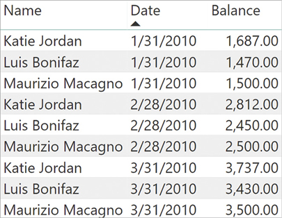
The sample data shows that the balance of Katie Jordan at the end of January was 1,687.00, whereas at the end of February the balance was 2,812.00. When we look at January and February together, her balance is not the sum of the two values. Instead, it is the last balance available. On the other hand, the overall balance of all customers in January is the sum of the three customers together.
If one uses a simple sum to aggregate values, the result of the calculation would be a sum over all the attributes as you can see in Figure 8-22.
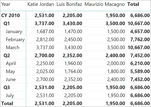
As you can note, the individual month values are correct. But at the aggregated levels—both at the quarter level and at the year level—the result is still a sum, making no sense. The correct result is visible in Figure 8-23, where—at each aggregate level—the report shows the last known value.
The handling of semi-additive measures is a complex topic, both because of the different possible calculations and because of the need to pay attention to several details. In the next sections we describe the basic techniques to handle semi-additive calculations.
Using LASTDATE and LASTNONBLANK
DAX offers several functions to handle semi-additive calculations. However, writing the correct code to handle semi-additive calculations is not just a matter of finding the correct function to use. Many subtle details might break a calculation if the author is not paying attention. In this section, we demonstrate different versions of the same code, which will or will not work depending on the data. The purpose of showing “wrong” solutions is educational because the “right” solution depends on the data present in the data model. Also, the solution of more complex scenarios requires some step-by-step reasoning.
The first function we describe is LASTDATE. We used the LASTDATE function earlier, when describing how to compute the moving annual total. LASTDATE returns a table only containing one row, which represents the last date visible in the current filter context. When used as a filter argument of CALCULATE, LASTDATE overrides the filter context on the date table so that only the last day of the selected period remains visible. The following code computes the last balance by using LASTDATE to overwrite the filter context on Date:
LastBalance :=
CALCULATE (
    SUM ( Balances[Balance] ),
    LASTDATE ( 'Date'[Date] )
)
LASTDATE is simple to use; unfortunately, LASTDATE is not the correct solution for many semi-additive calculations. In fact, LASTDATE scans the date table always returning the last date in the date table. For example, at the month level it always returns the last day of the month, and at the quarter level it returns the last date of the quarter. If the data is not available on the specific date returned by LASTDATE, the result of the calculation is blank. You see this in Figure 8-24 where the total of Q3 and the grand total are not visible. Because the total of Q3 is empty, the report does not even show Q3, resulting in a confusing result.

If, instead of using the month to slice data at the lowest level, we use the date, then the problem of LASTDATE becomes even more evident, as you can see in Figure 8-25. The Q3 row now is visible, even though its result is still blank.
If there are values on dates prior to the last day of the Date table, and that last day has no data available, then a better solution is to use the LASTNONBLANK function. LASTNONBLANK is an iterator that scans a table and returns the last value of the table for which the second parameter does not evaluate to BLANK. In our example, we use LASTNONBLANK to scan the Date table searching for the last date for which there are rows in the Balances table:
LastBalanceNonBlank :=
CALCULATE (
    SUM ( Balances[Balance] ),
    LASTNONBLANK (
        'Date'[Date],
        COUNTROWS ( RELATEDTABLE ( Balances ) )
    )
)
When used at the month level, LASTNONBLANK iterates over each date in the month, and for each date it checks whether the related table with the balances is empty. The innermost RELATEDTABLE function is executed in the row context of the LASTNONBLANK iterator, so that RELATEDTABLE only returns the balances of the given date. If there is no data, then RELATEDTABLE returns an empty table and COUNTROWS returns a blank. At the end of the iteration, LASTNONBLANK returns the last date that computed a nonblank result.
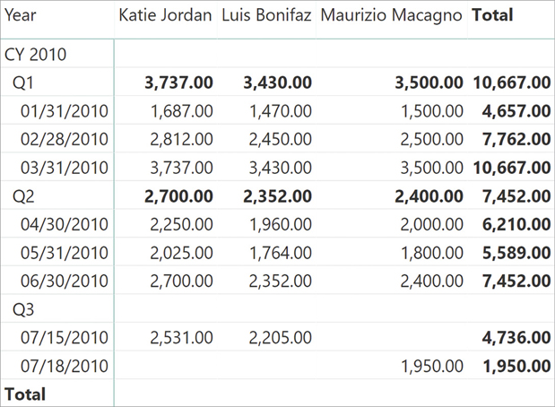
If all customer balances are gathered on the same date, then LASTNONBLANK solves the problem. In our example, we have different dates for different customers within the same month and this creates another issue. As we anticipated at the beginning of this section, with semi-additive calculations the devil is in the details. With our sample data LASTNONBLANK works much better than LASTDATE because it actively searches for the last date. However, it fails in computing correct totals, as you can see in Figure 8-26.

The result for each individual customer looks correct. Indeed, the last known balance for Katie Jordan is 2,531.00, which the formula correctly reports as her total. The same behavior produces correct results for Luis Bonifaz and Maurizio Macagno. Nevertheless, the grand total seems wrong. Indeed, the grand total is 1,950.00, which is the value of Maurizio Macagno only. It is confusing for a report to show a total composed in theory of three values (2,531.00, 2,205.00, 1,950.00) that only sums up the last value.
The reason is not hard to explain. When the filter context filters Katie Jordan, the last date with some values is July 15. When the filter context filters Maurizio Macagno, the last date becomes July 18. Nevertheless, when the filter context no longer filters the customer name, then the last date is Maurizio Macagno’s, which is July 18. Neither Katie Jordan nor Luis Bonifaz have any data on July 18. Therefore, for the month of July the formula only reports the value of Maurizio Macagno.
As it often happens, there is nothing wrong with the behavior of DAX. The problem is that our code is not complete yet because it does not consider the fact that different customers might have different last dates in our data model.
Depending on the requirements, the formula can be corrected in different ways. Indeed, one needs to define exactly what to show at the total level. Given the fact that there is some data on July 18, the idea is to either
Consider July 18 the last date to use for all the customers, regardless of their individual last date. Therefore, the customers not reported at a certain date have a zero balance at that date.
Consider each customer’s own last date, then aggregate the grand total using as the last date, the last date of each customer. Thus, the balance account of a customer is always the last balance available for that customer.
Both these definitions are correct, and it all depends on the requirements of the report. Because both are interesting to learn, we demonstrate how to write the code for both. The easier of the two is considering the last date for which there is some data regardless of the customer. The correct formula only requires changing the way LASTNONBLANK computes its result:
LastBalanceAllCustomers :=
VAR LastDateAllCustomers =
CALCULATETABLE (
LASTNONBLANK (
'Date'[Date],
COUNTROWS ( RELATEDTABLE ( Balances ) )
),
ALL ( Balances[Name] )
)
VAR Result =
CALCULATE (
SUM( Balances[Balance] ),
LastDateAllCustomers
)
RETURN
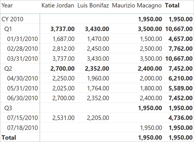
ResultIn this code we used CALCULATETABLE to remove the filter from the customer name during the evaluation of LASTNONBLANK. In this case, at the grand total LASTNONBLANK always returns July 18 regardless of the customer in the filter context. As a result, now the grand total adds up correctly, and the end balance of Katie Jordan and Luis Bonifaz is blank, as you can see in Figure 8-27.
The second option requires more complex reasoning. When using a different date for each customer, the grand total cannot be computed by simply using the filter context at the grand total. The formula needs to compute the subtotal of each customer and then aggregate the results. This is one of the scenarios where iterators are a simple and effective solution. Indeed, the following measure uses an outer SUMX to produce the total by summing the individual values of each customer:
LastBalanceIndividualCustomer :=
SUMX (
    VALUES ( Balances[Name] ),
    CALCULATE (
        SUM ( Balances[Balance] ),
        LASTNONBLANK (
            'Date'[Date],
            COUNTROWS ( RELATEDTABLE ( Balances ) )
        )
    )
)
The result of this latter measure computes for each customer the value on their own last date. It then aggregates the grand total by summing individual values. You see the result in Figure 8-28.

![]() Note
Note
With a large number of customers, the LastBalanceIndividualCustomer measure might have performance issues. The reason is that the formula includes two nested iterators, and the outer iterator has a large granularity. A faster approach to this same requirement is included in Chapter 10, “Working with the filter context,” leveraging functions like TREATAS that will be discussed in later chapters.
As you have learned, the complexity of semi-additive calculations is not in the code, but rather in the definition of its desired behavior. Once the behavior is clear, the choice between one pattern and the other is simple.
In this section we showed the most commonly used LASTDATE and LASTNONBLANK functions. There are two similar functions available to obtain the first date instead of the last date within a time period. These functions are FIRSTDATE and FIRSTNONBLANK. Moreover, there are further functions whose goal is to simplify calculations like the one demonstrated so far. We discuss them in the next section.
Working with opening and closing balances
DAX offers many functions like LASTDATE that simplify calculations retrieving the value of a measure at the opening or closing date of a time period. Although useful, these additional functions suffer from the same limitations as LASTDATE. That is, they work well if and only if the dataset contains values for all the dates.
These functions are STARTOFYEAR, STARTOFQUARTER, STARTOFMONTH, and the corresponding closing functions: ENDOFYEAR, ENDOFQUARTER, ENDOFMONTH. Intuitively, STARTOFYEAR always returns January 1 of the currently selected year in the filter context. In a similar way STARTOFQUARTER and STARTOFMONTH return the beginning of the quarter or of the month, respectively.
As an example, we prepared a different dataset that is aimed at resolving a different scenario where semi-additive calculations are useful. The demo file contains the prices of the Microsoft stock between 2013 and 2018. The value is well known at the day level. But what should a report show at an aggregated level—for example, at the quarter level? In this case, the most commonly used value is the last value of the stock price. In other words, stock prices are another example where the semi-additive pattern becomes useful.
A simple implementation of the last value of a stock works well for simple reports. The following formula computes the last value of the Microsoft stock, considering an average of the prices in case there are multiple rows for the same day:
Last Value :=
CALCULATE (
    AVERAGE ( MSFT[Value] ),
    LASTDATE ( 'Date'[Date] )
)
The result is correct when used in a daily chart like Figure 8-29.
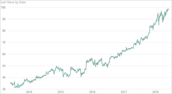
However, this nice result is not due to the DAX code working well. The chart looks correct because we used the date level in the x axis, and the client tool—Power BI in this example—works hard to ignore all the empty values in our dataset. This results in a continuous line. But using the same measure in a matrix sliced by year and month would make the gaps in the calculation become much more evident. This shows in Figure 8-30.

Using LASTDATE means you can expect empty values whenever there is no value on the exact last day of the month. That day might be either a weekend or a holiday. The correct version of Last Value is the following:
Last Value :=
CALCULATE (
    AVERAGE ( MSFT[Value] ),
    LASTNONBLANK (
        'Date'[Date],
        COUNTROWS ( RELATEDTABLE ( MSFT ) )
    )
)
Being mindful with these functions can prevent unexpected results. For example, imagine computing the Microsoft stock increase from the beginning of the quarter. One option, which again proves to be wrong, is the following code:
SOQ :=
CALCULATE (
    AVERAGE ( MSFT[Value] ),
    STARTOFQUARTER ( 'Date'[Date] )
)

SOQ% :=
DIVIDE (
    [Last Value] - [SOQ],
    [SOQ]
)
STARTOFQUARTER returns the date when the current quarter started, regardless the presence of data on that specific date. For example, January 1, which is the start of the first quarter, is also New Year’s Day. Consequently, there is never a price for a stock on that date, and the previous measures produce the result visible in Figure 8-31.
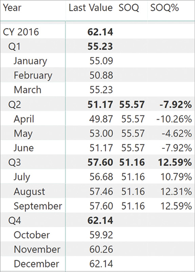
You can note that there are no values for SOQ in the first quarter. Besides, the issue is present for any quarter that starts on a day for which there is no data. To compute the start or the end of a time period, only taking into account dates with data available, the functions to use are FIRSTNONBLANK and LASTNONBLANK mixed with other time intelligence functions like, for example, DATESINPERIOD.
A much better implementation of the SOQ calculation is the following:
SOQ :=
VAR FirstDateInQuarter =
CALCULATETABLE (
FIRSTNONBLANK (
'Date'[Date],
COUNTROWS ( RELATEDTABLE( MSFT ) )
),
PARALLELPERIOD ( 'Date'[Date], 0, QUARTER )
)
VAR Result =
CALCULATE (
AVERAGE ( MSFT[Value] ),
FirstDateInQuarter
)
RETURN
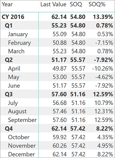
ResultThis latter version is much more complex both to author and to understand. However, it works in any scenario by only considering dates with data available. You can see the result of the matrix with the new implementation of SOQ in Figure 8-32.
At the risk of seeming pedantic, it is worth repeating the same concept used when introducing the topic of semi-additive measures. The devil is in the details. DAX offers several functions that work for models with data for all the dates. Unfortunately, not all models contain data for all the dates. In those latter scenarios, it is always extremely important to consider all the possible implications of using these simple functions. One should consider time intelligence functions as building blocks for more complex calculations. Combining different time intelligence functions enables the accurate computing of different time periods, although there is no predefined function solving the problem in a single step.
This is why instead of just showing you a smooth example for each time intelligence function, we preferred walking them through different trial-and-error scenarios. The goal of this section—and of the whole book—is not to just show you how to use functions. The goal is to empower you to think in DAX, to identify which details you should take care of, and to build your own calculations whenever the basic functionalities of the language are not enough for your needs.
In the next section we move one step forward in that same direction, by showing how most time intelligence calculations can be computed without the aid of any time intelligence functions. The goal is not purely educational. When working with custom calendars, such as weekly calendars, time intelligence functions are not useful. You need to be prepared to author some complex DAX code to obtain the desired result.
Understanding advanced time intelligence calculations
This section describes many important details about time intelligence functions. To showcase these details, we write time intelligence calculations by using simpler DAX functions such as FILTER, ALL, VALUES, MIN, and MAX. The goal of this section is not to suggest you avoid standard time intelligence functions in favor of simpler functions. Instead, the goal is to help you understand the exact behavior of time intelligence functions even in particular side cases. This knowledge enables you to then write custom calculations whenever the available functions do not provide the exact calculation you need. You will also notice that the translation to simpler DAX sometimes requires more code than expected because of certain hidden functionalities in time intelligence calculations.
Your reason for rewriting a time intelligence calculation in DAX could be that you are dealing with a nonstandard calendar, where the first day of the year is not always the same for all the years. This is the case, for example, for ISO calendars based on weeks. Here the assumption made by the time intelligence function that year, month, and quarter can always be extracted from the date value is no longer true. You can write a different logic by changing the DAX code in the filter conditions; or you can simply take advantage of other columns in the date table, so you do not have a complex DAX expression to maintain. You will find more examples of this latter approach under “Working with custom calendars” later in this chapter.
Understanding periods to date
Earlier, we described the DAX functions that calculate month-to-date, quarter-to-date, and year-to-date: they are DATESMTD, DATESQTD, and DATESYTD. Each of these filter functions is like the result of a FILTER statement that can be written in DAX. For example, consider the following DATESYTD function:
DATESYTD ( 'Date'[Date] )
It corresponds to a filter over the date column using FILTER called by CALCULATETABLE, as in the following code:
CALCULATETABLE (
    VAR LastDateInSelection = MAX ( 'Date'[Date] )
    RETURN
        FILTER (
            ALL ( 'Date'[Date] ),
            'Date'[Date] <= LastDateInSelection
                && YEAR ( 'Date'[Date] ) = YEAR ( LastDateInSelection )
        )
)
In a similar way, the DATESMTD function:
DATESMTD ( 'Date'[Date] )
corresponds to the following code:
CALCULATETABLE (
    VAR LastDateInSelection = MAX ( 'Date'[Date] )
    RETURN
        FILTER (
            ALL ( 'Date'[Date] ),
            'Date'[Date] <= LastDateInSelection
                && YEAR ( 'Date'[Date] ) = YEAR ( LastDateInSelection )
                && MONTH ( 'Date'[Date] ) = MONTH ( LastDateInSelection )
        )
)
The DATESQTD function follows the same pattern. All these alternative implementations have a common characteristic: They extract the information about year, month, and quarter from the last day available in the current selection. Then, they use this date to create a suitable filter.
The CALCULATETABLE generated for the column reference used in time intelligence functions is important when you have a row context. Look at the following two calculated columns, both created in the Date table:
'Date'[CountDatesYTD] = COUNTROWS ( DATESYTD ( 'Date'[Date] ) )

'Date'[CountFilter] =
COUNTROWS (
    VAR LastDateInSelection =
        MAX ( 'Date'[Date] )
    RETURN
        FILTER (
            ALL ( 'Date'[Date] ),
            'Date'[Date] <= LastDateInSelection
                && YEAR ( 'Date'[Date] ) = YEAR ( LastDateInSelection )
        )
)
Though they look similar, they are not. Indeed, you can see the result in Figure 8-33.
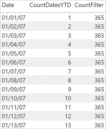
CountDatesYTD returns the number of days from the beginning of the year, up to the date in the current row. To achieve this result, DATESYTD should inspect the current filter context and extract the selected period from the filter context. However, being computed in a calculated column, there is no filter context. The behavior of CountFilter is simpler to explain: When CountFilter computes the maximum date, it always retrieves the last date of the entire date table because there are no filters in the filter context. CountDatesYTD behaves differently because DATESYTD performs a context transition being called with a date column reference. Thus, it creates a filter context that only contains the currently iterated date.
If you rewrite DATESYTD and you know that the code will not be executed inside a row context, you can remove the outer CALCULATETABLE, which would otherwise be a useless operation. This is usually the case for a filter argument in a CALCULATE call not called within an iterator—a place where DATESYTD is often used. In these cases, instead of DATESYTD, you can write:
VAR LastDateInSelection = MAX ( 'Date'[Date] )
RETURN
    FILTER (
        ALL ( 'Date'[Date] ),
        'Date'[Date] <= LastDateInSelection
            && YEAR ( 'Date'[Date] ) = YEAR ( LastDateInSelection )
    )
On the other hand, to retrieve the date from the row context—for example, in a calculated column—it is easier to retrieve the date value of the current row in a variable instead of using MAX:
VAR CurrentDate = 'Date'[Date]
RETURN
    FILTER (
        ALL ( 'Date'[Date] ),
        'Date'[Date] <= CurrentDate
            && YEAR ( 'Date'[Date] ) = YEAR ( CurrentDate )
    )
DATESYTD allows the specifying of a year-end date, which is useful to compute YTD on fiscal years. For example, for a fiscal year starting on July 1, June 30 needs to be specified in the second argument by using one of the following versions:
DATESYTD ( 'Date'[Date], "06-30" )
DATESYTD ( 'Date'[Date], "30-06" )
Regardless of the local culture, let us assume that the programmer has specified the <month> and <day>. The corresponding FILTER of DATESYTD using these placeholders is the following:
VAR LastDateInSelection = MAX ( 'Date'[Date] )
RETURN
    FILTER (
        ALL ( 'Date'[Date] ),
        'Date'[Date] > DATE ( YEAR ( LastDateInSelection ) - 1, <month>, <day> )
            && 'Date'[Date] <= LastDateInSelection
)![]() Important
Important
It is important to note that DATESYTD always starts from the day after the specified end of the fiscal year. This causes a problem in the special case where a company has a fiscal year starting on March 1. In fact, the end of the fiscal year can be either February 28 or 29, depending on whether the calculation is happening in a leap year or not. As of April 2019, this special scenario is not supported by DATESYTD. Thus, if one needs to author code and they have to start the fiscal calendar on March 1, then DATESYTD cannot be used. A workaround is available at http://sql.bi/fymarch.
Understanding DATEADD
DATEADD retrieves a set of dates shifted in time by a certain offset. When DATEADD analyzes the current filter context, it includes special handling to detect whether the current selection is one month or a special period, like the beginning or the end of a month. For example, when DATEADD retrieves an entire month shifted back one quarter, it oftentimes returns a different number of days than the current selection. This happens because DATEADD understands that the current selection is a month, and it retrieves a full corresponding month regardless of the number of days.
These special behaviors are expressed in three rules that we describe in this section. These rules make it hard to rewrite DATEADD on a generic date table. The code would be painfully difficult to write and nearly impossible to manage over time. DATEADD only uses the values of the date column, extracting the information needed—such as year, quarter, and month—from the available date value. The same logic would be hard to reproduce in plain DAX. On the other hand, by using additional columns in the Date table, one can author an alternative version of DATEADD. We will elaborate on this technique later in this chapter, in the section about custom calendars.
Consider the following formula:
DATEADD ( 'Date'[Date], -1, MONTH )
The closest—but not totally equivalent—DAX formula is the following:
VAR OffsetMonth = -1
RETURN TREATAS (
    SELECTCOLUMNS (
        CALCULATETABLE ( DISTINCT ( 'Date'[Date] ) ),
        "Date", DATE (
            YEAR ( 'Date'[Date] ),
            MONTH ( 'Date'[Date] ) + OffsetMonth,
            DAY ( 'Date'[Date] )
        )
    ),
    'Date'[Date]
)![]() Note
Note
In the previous example and in other formulas in this chapter, we use the TREATAS function, which applies a table expression to the filter context on the columns specified by the second and following arguments. You can read a more complete description of this function in Chapter 10.
The formula also works in January because a value lower than 1 for the month parameter is considered an offset to go into a previous year. However, this implementation only works properly if the destination month has the same number of days as the current month. If you move from February to January, the formula misses two or three days, depending on the year. In a similar way, if you move from March to February, the result might include days in March.
On the other hand, DATEADD does not have a similar problem and returns the entire month with the offset applied, in case an entire month was selected before the offset was applied. In order to achieve this, DATEADD uses three rules:
DATEADD only returns days that exist in the date column. If some expected dates are missing, then DATEADD returns only those dates that are not missing in the date column.
If a day does not exist in the corresponding month after the shifting operation, then the result of DATEADD includes the last day of the corresponding month.
If the selection includes the last two days of a month, then the result of DATEADD includes all the days between the corresponding days in the shifted month and the end of the shifted month.
A few examples are helpful to understand the effects of these behaviors. Consider the following measures: Day count counts the number of selected days; PM Day count counts the number of days shifted back in the previous month; PM Range returns the date range selected by DATEADD.
Day count :=
COUNTROWS ( 'Date' )

PM Day count :=
CALCULATE ( [Day count], DATEADD ( 'Date'[Date], -1, MONTH ) )

PM Range :=
CALCULATE (
    VAR MinDate = MIN ( 'Date'[Date] )
    VAR MaxDate = MAX ( 'Date'[Date] )
    VAR Result =
        FORMAT ( MinDate, "MM/DD/YYYY - " ) & FORMAT ( MaxDate, "MM/DD/YYYY" )
    RETURN
        Result,
    DATEADD ( 'Date'[Date], -1, MONTH )
)
Rule 1 is in effect when the selection is near the boundaries of the range of dates included in the date column. For example, Figure 8-34 shows the PM Day count and PM Range measures returning valid values in February 2007 because dates in January 2007 exist in the date column, whereas the same measures return blanks in January 2007 because dates in December 2006 are not present in the date column.

Figure 8-34 The dates selected are shifted back one month. The main reason why the Date table should include all the days within one year is because of the behavior of DATEADD. Be mindful that several time intelligence functions in DAX internally use DATEADD. Therefore, having a complete date table is of paramount importance for DAX time intelligence functions to behave as expected.
Rule 2 is relevant because months have different numbers of days. The 31st day does not exist for all months. If it is selected, it is moved to the last day of the month in the shifted period. For example, in Figure 8-35 the last days of March are all moved to the last day of February because February 29 to 31 do not exist in 2007.
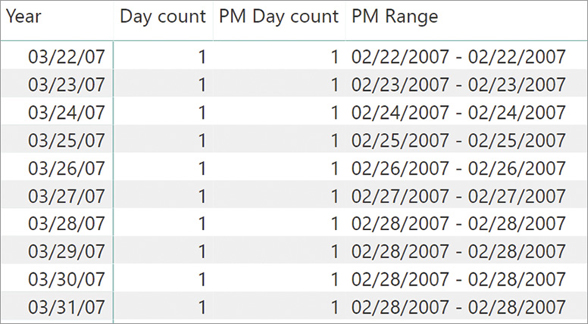
Figure 8-35 A date that does not exist in the destination month is replaced by the last day of the destination month. The consequence of this rule is that you might obtain a lower number of days than the initial selection. This is intuitive when the selection of 31 days in March should result in a corresponding selection of 28 or 29 days in February. However, when the selection includes a reduced number of days, the result might not be what is expected. For example, in Figure 8-36 you can see that a selection of 5 days in March 2007 results in only 2 days in February 2007.
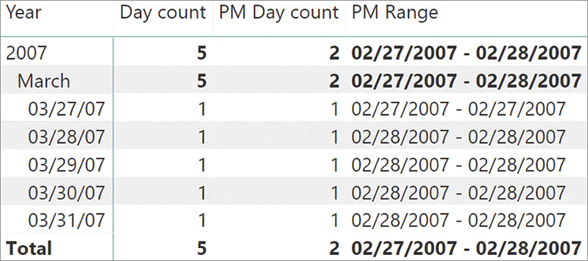
Figure 8-36 Several days in the starting selection might result in the same day in the DATEADD result. Rule 3 generates a special handling type when the last day of a month is included within a range of dates. For example, consider the initial selection of three days from June 29, 2007, to July 1, 2007. The selection only includes three days, but among those is the last day of June, which is June 30. When DATEADD shifts the dates back, it includes the last day of May (May 31). Figure 8-37 shows this behavior and it is worth a deeper look. Indeed, you can note that June 30 is moved to May 30. Only if the selection contains both June 29 and 30 does the result then include the last day of the previous month (May 31). In this case, the number of days in the previous month is greater than the number of days originally selected: 2 days selected in June 2017 return 3 days in the previous month (May 2007).
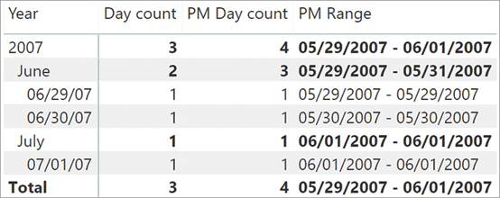
Figure 8-37 The result of DATEADD includes all days between the first and the last day of the selection after the shift operation.
The reason for these rules is to provide an intuitive behavior when a formula operates at the month level. As you can see in Figure 8-38, when you compare the selections at the month level, the result is intuitive and expected. It shows the complete range of days of the previous month.

Understanding the rules described in this section is important to handle side conditions that might happen with partial selections of days in months. For example, consider a filter over weekdays in a report. That filter might not include the last days of a month, which would guarantee that the entire previous month is selected. Moreover, the shift of dates performed by DATEADD only considers the number of days within the month and not the week days. The application of a filter to the date column of the Date table also generates an implicit ALL over the Date table itself, removing any existing filter over other columns of the Date table including weekdays. Thus, a slicer that filters weekdays is not compatible with the use of DATEADD because it does not produce the expected result.
For example, consider the following definition of PM Sales DateAdd displaying the Sales Amount of the previous month, as shown in Figure 8-39:
PM Sales DateAdd :=
CALCULATE (
    [Sales Amount],
    DATEADD ( 'Date'[Date], -1, MONTH )
)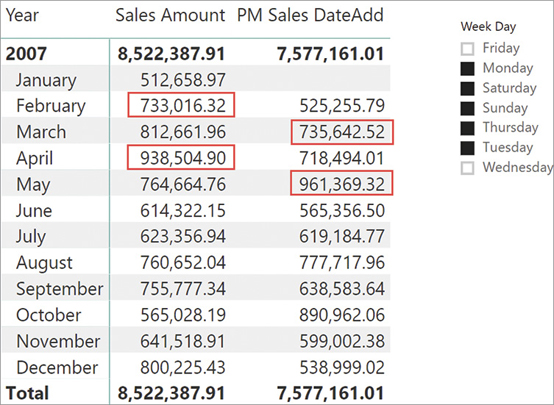
PM Sales DateAdd creates a filter of days that does not correspond to the full month. It translates the days of the month selected, including additional days at the end of the month according to Rule 3. This filter overrides and ignores the Day of Week selection for the value of the previous month. The result produces different values, even bigger than Sales Amount as in March and May 2007, for example.
In this case, computing correctly requires a custom calculation like the one implemented in the PM Sales Weekday measure. It applies a filter over the YearMonthNumber column keeping the filter on Day of Week, and removing the filter from all the other columns of the Date table using ALLEXCEPT. The YearMonthNumber calculated column is a sequential number over months and years:
Date[YearMonthNumber] =
'Date'[Year] * 12 + 'Date'[Month Number] - 1

PM Sales Weekday :=
VAR CurrentMonths = DISTINCT ( 'Date'[YearMonthNumber] )
VAR PreviousMonths =
    TREATAS (
        SELECTCOLUMNS (
            CurrentMonths,
            "YearMonthNumber", 'Date'[YearMonthNumber] - 1
        ),
        'Date'[YearMonthNumber]
    )
VAR Result =
    CALCULATE (
        [Sales Amount],
        ALLEXCEPT ( 'Date', 'Date'[Week Day] ),
        PreviousMonths
    )
RETURN
    Result
The result is visible in Figure 8-40.
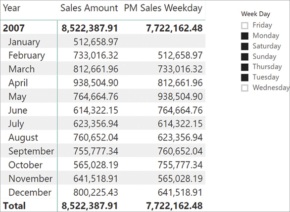
However, this solution works specifically for this report. If the selection of days were made based on other criteria like the first 6 days of the month, then the result produced by PM Sales Weekday would get the entire month, whereas the result produced by PM Sales DateAdd would work in this case. Depending on the columns visible to the user, one might implement different calculations based on the selection made. For example, the following PM Sales measure uses the ISFILTERED function to check whether a filter is active on the Day of Week column. A more detailed explanation of ISFILTERED is included in Chapter 10.
PM Sales :=
IF (
    ISFILTERED ( 'Date'[Day of Week] ),
    [PM Sales Weekday],
    [PM Sales DateAdd]
)
Understanding FIRSTDATE, LASTDATE, FIRSTNONBLANK, and LASTNONBLANK
In the “Understanding semi-additive calculations” section earlier in this chapter, you learned two functions that seem alike: LASTDATE and LASTNONBLANK. In fact, these functions exhibit distinctive behaviors, and so do the two companions FIRSTDATE and FIRSTNONBLANK.
FIRSTDATE and LASTDATE only operate on a date column. They return, respectively, the first and the last date in the active filter context, ignoring any data existing in other related tables:
FIRSTDATE ( 'Date'[Date] )
LASTDATE ( 'Date'[Date] )
FIRSTDATE returns the minimum value of the column received in the current filter context, whereas LASTDATE returns the maximum value. FIRSTDATE and LASTDATE behave somewhat like MIN and MAX, with one important difference: FIRSTDATE and LASTDATE return a table and perform a context transition, whereas MIN and MAX return a scalar value without doing any context transition.
For example, consider the following expression:
CALCULATE (
    SUM ( Inventory[Quantity] ),
    LASTDATE ( 'Date'[Date] )
)
You can rewrite the formula using MAX instead of LASTDATE, but this would result in unnecessary longer code:
CALCULATE (
    SUM ( Inventory[Quantity] ),
    FILTER (
        ALL ( 'Date'[Date] ),
        'Date'[Date] = MAX ( 'Date'[Date] )
    )
)
Besides, LASTDATE also performs a context transition. Consequently, the exact equivalent of LASTDATE in plain DAX is as follows:
CALCULATE (
    SUM ( Inventory[Quantity] ),
    VAR LastDateInSelection =
        MAXX ( CALCULATETABLE ( DISTINCT ( 'Date'[Date] ) ), 'Date'[Date] )
    RETURN
        FILTER (
            ALL ( 'Date'[Date] ),
            'Date'[Date] = LastDateInSelection
        )
)
The context transition is relevant when you execute FIRSTDATE/LASTDATE in a row context. The best practice is to use FIRSTDATE/LASTDATE when you write a filter expression because a table expression is expected, whereas MIN/MAX functions are better when you are writing a logical expression in a row context that usually requires a scalar value. Indeed, LASTDATE with a column reference implies a context transition that hides the external filter context.
For example, you will favor FIRSTDATE/LASTDATE over MIN/MAX in a filter argument of CALCULATE/CALCULATETABLE functions because the syntax is simpler. However, you should use MIN/MAX when the context transition implied by FIRSTDATE/LASTDATE would modify the result. This is the case of the condition in a FILTER function. The following expression filters the dates for computing a running total:
FILTER (
    ALL ( 'Date'[Date] ),
    'Date'[Date] <= MAX ( 'Date'[Date] )
)
MAX is the right function to use. In fact, the result of using LASTDATE instead of MAX would always contain all the dates, regardless of the current selection because of the unwanted context transition. Thus, the following expression returns all dates, no matter what. The reason is that LASTDATE—because of context transition—returns the value of Date[Date] in each row of the FILTER iteration:
FILTER (
    ALL ( 'Date'[Date] ),
    'Date'[Date] <= LASTDATE ( 'Date'[Date] ) -- this condition is always true
)
LASTNONBLANK and FIRSTNONBLANK are different from FIRSTDATE and LASTDATE. In fact, LASTNONBLANK and FIRSTNONBLANK are iterators, meaning that they scan a table row by row in a row context and that they return the last (or first) of the values for which the second parameter is not a blank. Usually, the second parameter of these functions is either a measure or an expression including CALCULATE, so to rely on context transition.
To obtain the right value for the last non-blank date for a given measure/table, you use an expression like this:
LASTNONBLANK ( 'Date'[Date], CALCULATE ( COUNTROWS ( Inventory ) ) )
It returns the last date (in the current filter context) for which there are rows in the Inventory table. You can also use an equivalent formula:
LASTNONBLANK ( 'Date'[Date], COUNTROWS ( RELATEDTABLE ( Inventory ) ) )
That last expression returns the last date (in the current filter context) for which there is a related row in the Inventory table.
It is worth noting that FIRSTNONBLANK/LASTNONBLANK functions accept any data type as their first argument, whereas the FIRSTDATE/LASTDATE functions require a column of DateTime or Date data type. Thus, and though it is not a commonly used practice, FIRSTNONBLANK and LASTNONBLANK can also be used with different tables like customers, products, or any other table.
Using drillthrough with time intelligence
A drillthrough operation is a request for the data source rows corresponding to the filter context used in a certain calculation. Every time you use a time intelligence function, you change the filter context on the Date table. This produces a different result for the measure from the result obtained with the initial filter context. When you use a client that performs a drillthrough action over a report, such as a pivot table in Excel, you could observe a behavior that is not what you might expect. In fact, the drillthrough operation made in MDX does not consider the changes in the filter context defined by the measure itself. Instead, it only considers the filter context defined by the rows, columns, filters, and slicers of the pivot table.
For example, by default the drillthrough on March 2007 always returns the same rows, regardless of the time intelligence function applied in the measure. By using TOTALYTD, one would expect all the days from January to March 2007; by using SAMEPERIODLASTYEAR, one would expect March 2006; and by using LASTDATE, one would only expect the rows for March 31, 2007. Indeed, in the default drillthrough any of these filters always returns all the rows for March 2007. This behavior can be controlled by the Detail Rows property in the Tabular model. At the time of writing (April 2019), the Detail Rows property can be set in an Analysis Services 2017 or Azure Analysis Services data model, but it is not available either in Power BI or in Power Pivot for Excel.
The Detail Rows property must apply the same filter used for the corresponding time intelligence measure. For example, consider the following year-to-date measure:
CALCULATE (
    [Sales Amount],
    DATESYTD ( 'Date'[Date] )
)
Its Detail Rows property should be set to
CALCULATETABLE (
    Sales,                       -- This expression also controls the columns returned
    DATESYTD ( 'Date'[Date] )
)
Working with custom calendars
As you have seen so far, the standard time intelligence functions in DAX only support standard Gregorian calendars. These are based on a solar calendar divided into 12 months, each one with a different number of days. These functions work well to analyze data by year, quarter, month, and day. However, there are models that have a different definition of time periods, like week-based calendars such as the ISO week date system. If someone needs a custom calendar, they need to rewrite the time intelligence logic in DAX because the standard time intelligence calculation would be of no use.
When it comes to nonstandard calendars, there are so many variations that it would be impossible to cover them all. Therefore, we show examples of how to implement time intelligence calculations in DAX when you cannot use standard functions.
In order to simplify the formulas, a common technique is to move part of the business logic in the date table through the use of dedicated columns. The standard DAX time intelligence functions do not use any information from the date table other than the date column. This is a design choice of DAX because this way the behavior of the language does not depend on the presence of additional metadata to identify columns to determine year, quarter, and month of a date—as was the case with MDX and Analysis Services Multidimensional. Being the owner of your model and of your DAX code, you can make more assumptions, and this helps in simplifying the code to handle custom time-related calculations.
This final section shows a few examples of the formulas for custom calendars. If needed, you can find more information, examples, and ready-to-use DAX formulas in the following articles:
Time Patterns: http://www.daxpatterns.com/time-patterns/
Week-Based Time Intelligence in DAX: http://sql.bi/isoweeks/
Working with weeks
DAX does not provide any time intelligence functions that handle weeks. The reason is that there are many different standards and techniques to define weeks within a year, and to define the notion of calculation over weeks. Oftentimes a single week crosses the boundaries of years, quarters, and months. You need to write the code to handle your own definition of a week-based calendar. For example, in ISO a week-date system of January 1 and January 2 in 2011 belongs to week 52 of year 2010, and the first week of 2011 starts on January 3.
Although there are different standards, you can learn a generic approach that should work in most cases. The approach involves the creation of additional columns in the Date table to store the relationship between weeks and their month/quarter/year. Changing the association rules will just require changing the content of the Date table, without modifying the DAX code of the measures.
For example, you can extend a Date table to support ISO weeks by using the following calculated columns:
'Date'[Calendar Week Number] = WEEKNUM ( 'Date'[Date], 1 )

'Date'[ISO Week Number] = WEEKNUM ( 'Date'[Date], 21 )

'Date'[ISO Year Number] = YEAR ( 'Date'[Date] + ( 3 - WEEKDAY ( 'Date'[Date], 3 ) ) )

'Date'[ISO Week] = "W" & 'Date'[ISO Week Number] & "-" & 'Date'[ISO Year Number]

'Date'[ISO Week Sequential] = INT ( ( 'Date'[Date] - 2 ) / 7 )

'Date'[ISO Year Day Number] =
VAR CurrentIsoYearNumber = 'Date'[ISO Year Number]
VAR CurrentDate = 'Date'[Date]
VAR DateFirstJanuary = DATE ( CurrentIsoYearNumber, 1, 1 )
VAR DayOfFirstJanuary = WEEKDAY ( DateFirstJanuary, 3 )
VAR OffsetStartIsoYear = - DayOfFirstJanuary + ( 7 * ( DayOfFirstJanuary > 3 ) )
VAR StartOfIsoYear = DateFirstJanuary + OffsetStartIsoYear
VAR Result = CurrentDate - StartOfIsoYear
RETURN
    Result
You can see in Figure 8-41 the result of these columns. The ISO Week column will be visible to users, whereas the ISO Week Sequential Number is for internal use only. ISO Year Day Number is the number of days since the beginning of the ISO year. These additional columns make it easy to compare different periods.
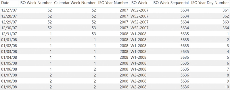
Using the new columns, a developer can write year-to-date aggregation by using the ISO Year Number column instead of extracting the year number from the date. This technique is the same as the one you learned in the “Understanding periods to date” section earlier in this chapter. We just added an additional check to make sure that only one ISO Year is selected, prior to invoking the VALUES function:
ISO YTD Sales :=
IF (
    HASONEVALUE ( 'Date'[ISO Year Number] ),
    VAR LastDateInSelection = MAX ( 'Date'[Date] )
    VAR YearSelected = VALUES ( 'Date'[ISO Year Number] )
    VAR Result =
        CALCULATE (
            [Sales Amount],
            'Date'[Date] <= LastDateInSelection,
            'Date'[ISO Year Number] = YearSelected,
            ALL ( 'Date' )
        )
    RETURN
        Result
)
Figure 8-42 shows the result of the ISO YTD Sales measure at the beginning of 2008, compared with a standard YTD computed through DATESYTD. The ISO version accurately includes December 31, 2007, which belongs to ISO Year 2008.
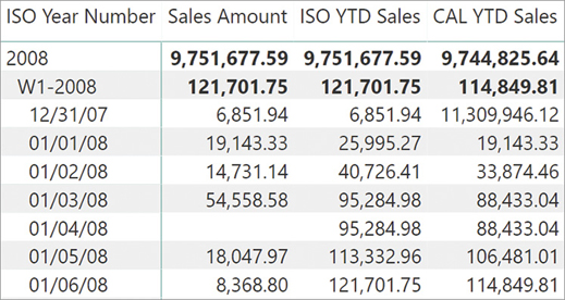
The comparison with the prior year should compare the relative weeks of the year with the same weeks in the previous year. Since the dates might be different, it is simpler to use other columns in the date table to implement the comparison logic. The distribution of weeks within each year is regular because each week always has seven days, whereas calendar months have different lengths and cannot benefit from the same assumption. In week-based calendars, you can simplify the calculation by looking in the previous year for the same relative days that were selected in the current filter context.
The following ISO PY Sales measure filters the same selection of days in the previous year. This technique also works when the selection includes complete weeks because the days are selected using the ISO Year Day Number value and not the effective date.
ISO PY Sales :=
IF (
    HASONEVALUE ( 'Date'[ISO Year Number] ),
    VAR DatesInSelection = VALUES ( 'Date'[ISO Year Day Number] )
    VAR YearSelected = VALUES ( 'Date'[ISO Year Number] )
    VAR PrevYear = YearSelected - 1
    VAR Result =
        CALCULATE (
            [Sales Amount],
            DatesInSelection,
            'Date'[ISO Year Number] = PrevYear,
            ALL ( 'Date' )
        )
    RETURN
        Result
)
Figure 8-43 shows the result produced by the ISO PY Sales measure. On the right we added the sales amount of 2007, to make it easier to understand the source of ISO PY Sales.

Week-based calendars are simple to manage because of the assumption you can make about the symmetry between days in different years. This is usually not compatible with the calendar month, so if you want to use both hierarchies (months and weeks), you should create different time intelligence calculations for each hierarchy.
Custom year-to-date, quarter-to-date, and month-to-date
Earlier in this chapter, you learned how to rewrite DATESYTD and similar functions in the “Understanding periods to date” section. There, we could still extract date attributes—like the year—from the date column. With ISO calendars, this logic is no longer in the date column. Instead, we created additional columns just for this calculation. In this section we now demonstrate how to replace the logic that extracts information from the date value by using other columns of the Date table.
For example, consider the following YTD Sales measure:
YTD Sales :=
CALCULATE (
    [Sales Amount],
    DATESYTD ( 'Date'[Date] )
)
The corresponding syntax in DAX without time intelligence is the following:
YTD Sales :=
VAR LastDateInSelection = MAX ( 'Date'[Date] )
VAR Result =
    CALCULATE (
        [Sales Amount],
        'Date'[Date] <= LastDateInSelection
           && YEAR ( 'Date'[Date] ) = YEAR ( LastDateInSelection )
    )
RETURN
    Result
If you use a custom calendar, you must replace the YEAR function call with an access to the Year column, such as in the following YTD Sales Custom measure:
YTD Sales Custom :=
VAR LastDateInSelection = MAX ( 'Date'[Date] )
VAR LastYearInSelection = MAX ( 'Date'[Calendar Year Number] )
VAR Result =
    CALCULATE (
        [Sales Amount],
        'Date'[Date] <= LastDateInSelection,
        'Date'[Calendar Year Number] = LastYearInSelection,
        ALL ( 'Date' )
    )
RETURN
    Result
You can use the same template to implement quarter-to-date and month-to-date calculations. The only difference is the column used instead of Calendar Year Number:
QTD Sales Custom :=
VAR LastDateInSelection = MAX ( 'Date'[Date] )
VAR LastYearQuarterInSelection = MAX ( 'Date'[Calendar Year Quarter Number] )
VAR Result =
    CALCULATE (
        [Sales Amount],
        'Date'[Date] <= LastDateInSelection,
        'Date'[Calendar Year Quarter Number] = LastYearQuarterInSelection,
        ALL ( 'Date' )
    )
RETURN
    Result

MTD Sales Custom :=
VAR LastDateInSelection = MAX ( 'Date'[Date] )
VAR LastYearMonthInSelection = MAX ( 'Date'[Calendar Year Month Number] )
VAR Result =
    CALCULATE (
        [Sales Amount],
        'Date'[Date] <= LastDateInSelection,
        'Date'[Calendar Year Month Number] = LastYearMonthInSelection,
        ALL ( 'Date' )
    )
RETURN
    Result
You can use these formulas to implement calculations for both standard calendars (in case you want to improve performance using DirectQuery) and custom calendars (in case the time periods are not standard periods).
Conclusions
In this long chapter, you learned the basics of time intelligence calculations in DAX. These are the important points we covered:
Both Power Pivot and Power BI have mechanisms to automate the creation of a date table. They are not worth using, unless your requirements are really simple. Having control over your date table is important and the existing tools do not let you modify the tables to follow your needs.
Building a date table is easy by leveraging CALENDARAUTO and some simple DAX code. It is worth investing some time to build your own date table, as you will reuse the code in many different projects. You can also download DAX templates for a date table on the web.
A data table should be marked as a date table to simplify the use of time intelligence calculations.
There are several time intelligence functions. Most of them simply return a table that can be used as a filter argument of CALCULATE.
You should learn to treat time intelligence functions as building blocks for more complex calculations. By mixing time intelligence functions, one can create several different and complex calculations.
When the requirements are such that standard time intelligence calculations no longer work, it is time to roll up your sleeves and learn to author time intelligence calculations with simpler DAX functions.
There are several examples of time intelligence calculations in this book. However, you can find many more at https://www.daxpatterns.com/time-patterns/.