
9. Improving Deep Networks
In Chapter 6, we detailed individual artificial neurons. In Chapter 7, we arranged these neural units together as the nodes of a network, enabling the forward propagation of some input x through the network to produce some output ŷ. Most recently, in Chapter 8, we described how to quantify the inaccuracies of a network (compare ŷ to the true y with a cost function) as well as how to minimize these inaccuracies (adjust the network parameters w and b via optimization with stochastic gradient descent and backpropagation).
In this chapter, we cover common barriers to the creation of high-performing neural networks and techniques that overcome them. We apply these ideas directly in code while architecting our first deep neural network.1 Combining this additional network depth with our newfound best practices, we’ll see if we can outperform the handwritten-digit classification accuracy of our simpler, shallower architectures from previous chapters.
1. Recall from Chapter 4 that a neural network earns the deep moniker if it consists of at least three hidden layers.
Weight Initialization
In Chapter 8, we introduced the concept of neuron saturation (see Figure 8.1), where very low or very high values of z diminish the capacity for a given neuron to learn. At the time, we offered cross-entropy cost as a solution. Although cross-entropy does effectively attenuate the effects of neuron saturation, pairing it with thoughtful weight initialization will reduce the likelihood of saturation occurring in the first place. As mentioned in a footnote in Chapter 1, modern weight initialization provided a significant leap forward in deep learning capability: It is one of the landmark theoretical advances between LeNet-5 (Figure 1.11) and AlexNet (Figure 1.17) that dramatically broadened the range of problems artificial neural networks could reliably solve. In this section, we play around with several weight initializations to help you develop an intuition around how they’re so impactful.
While describing neural network training in Chapter 8, we mentioned that the parameters w and b are initialized with random values such that a network’s starting approximation of y will be far off the mark, thereby leading to a high initial cost C. We haven’t needed to dwell on this much, because, in the background, Keras by default constructs TensorFlow models that are initialized with sensible values for w and b. It’s nevertheless worthwhile discussing this initialization, not only to be aware of another method for avoiding neuron saturation but also to fill in a gap in your understanding of how neural network training works. Although Keras does a sensible job of choosing default values—and that’s a key benefit of using Keras in the first place—it’s certainly possible, and sometimes even necessary, to change these defaults to suit your problem.
To make this section interactive, we encourage you to check out our accompanying Jupyter notebook, Weight Initialization. As shown in the following chunk of code, our library dependencies are NumPy (for numerical operations), matplotlib (for generating plots), and a handful of Keras methods, which we will detail as we work through them in this section.
import numpy as np
import matplotlib.pyplot as plt
from keras import Sequential
from keras.layers import Dense, Activation
from keras.initializers import Zeros, RandomNormal
from keras.initializers import glorot_normal, glorot_uniform
In this notebook, we simulate 784 pixel values as inputs to a single dense layer of artificial neurons. The inspiration behind our simulation of these 784 inputs comes of course from our beloved MNIST digits (Figure 5.3). For the number of neurons in the dense layer (256), we picked a number large enough so that, when we make some plots later on, they have ample data:
n_input = 784
n_dense = 256
Now for the impetus of this section: the initialization of the network parameters w and b. Before we begin passing training data into our network, we’d like to start with reasonably scaled parameters. This is for two reasons.
Large w and b values tend to correspond to larger z values and therefore saturated neurons (see Figure 8.1 for a plot on neuron saturation).
Large parameter values would imply that the network has a strong opinion about how x is related to y, but before any training on data has occurred, any such strong opinions are wholly unmerited.
Parameter values of zero, on the other hand, imply the weakest opinion on how x is related to y. To bring back the fairy tale yet again, we’re aiming for a Goldilocks-style, middle-of-the-road approach that starts training from a balanced and learnable beginning. With that in mind, when we design our neural network architecture, we select the Zeros() method for initializing the neurons of our dense layer with b = 0:
b_init = Zeros()
Following the line of thinking from the preceding paragraph to its natural conclusion, we might be tempted to think that we should also initialize our network weights w with zeros as well. In fact, this would be a training disaster: If all weights and biases were identical, many neurons in the network would treat a given input x identically, giving stochastic gradient descent a minimum of heterogeneity for identifying individual parameter adjustments that might reduce the cost C. It would be more productive to initialize weights with a range of different values so that each neuron treats a given x uniquely, thereby providing SGD with a wide variety of starting points for approximating y. By chance, some of the initial neuron outputs may contribute in part to a sensible mapping from x to y. Although this contribution will be weak at first, SGD can experiment with it to determine whether it might contribute to a reduction in the cost C between the predicted ŷ and the target y.
As worked through earlier (e.g., in discussion of Figures 7.5 and 8.9), the vast majority of the parameters in a typical network are weights; relatively few are biases. Thus, it’s acceptable (indeed, it’s the most common practice) to initialize biases with zeros, and the weights with a range of values near zero. One straightforward way to generate random values near zero is to sample from the standard normal distribution2 as in Example 9.1.
2. The normal distribution is also known as the Gaussian distribution or, colloquially, as the “bell curve” because of its bell-like shape. The standard normal distribution in particular is a normal distribution with a mean of 0 and standard deviation of 1.
Example 9.1 Weight initialization with values sampled from standard normal distribution
w_init = RandomNormal(stddev=1.0)
To observe the impact of the weight initialization we’ve chosen, in Example 9.2 we design a neural network architecture for our single dense layer of sigmoid neurons.
Example 9.2 Architecture for a single dense layer of sigmoid neurons
model = Sequential()
model.add(Dense(n_dense,
                input_dim=n_input,
                kernel_initializer=w_init,
                bias_initializer=b_init))
model.add(Activation('sigmoid'))
As in all of our previous examples, we instantiate a model by using Sequential(). We then use the add() method to create a single Dense layer with the following parameters:
256 neurons (
n_dense)784 inputs (
n_input)kernel_initializerset tow_initto initialize the network weights via our desired approach, in this case sampling from the standard normal distributionbias_initializerset tob_initto initialize the biases with zeros
For simplicity when updating it later in this section, we add the sigmoid activation function to the layer separately by using Activation('sigmoid').
With our network set up, we use the NumPy random() method to generate 784 “pixel values,” which are floats randomly sampled from the range [0.0, 1.0):
x = np.random.random((1,n_input))
We subsequently use the predict() method to forward propagate x through the single layer and output the activations a:
a = model.predict(x)
With our final line of code, we use a histogram to visualize the a activations:3
3. In case you’re wondering, the leading underscore (_ =) keeps the Jupyter notebook tidier by outputting the plot only, instead of the plot as well as an object that stores the plot.
_ = plt.hist(np.transpose(a))
Your result will look slightly different from ours because of the random() method we used to generate our input values, but your outputs should look approximately like those shown in Figure 9.1.
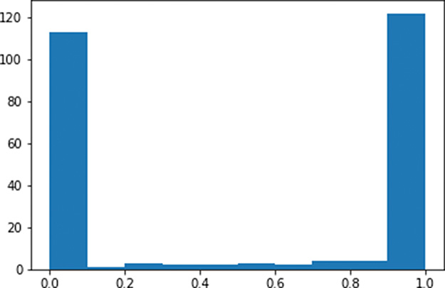
Figure 9.1 Histogram of the a activations output by a layer of sigmoid neurons, with weights initialized using a standard normal distribution
As expected given Figure 6.9, the a activations output from our sigmoid layer of neurons is constrained to a range from 0 to 1. What is undesirable about these activations, however, is that they are chiefly pressed up against the extremes of the range: Most of them are either immediately adjacent to 0 or immediately adjacent to 1. This indicates that with the normal distribution from which we sampled to initialize the layer’s weights w, we ended up encouraging our artificial neurons to produce large z values. This is unwelcome for two reasons mentioned earlier in this section:
It means the vast majority of the neurons in the layer are saturated.
It implies that the neurons have strong opinions about how x would influence y prior to any training on data.
Thankfully, this ickiness can be resolved by initializing our network weights with values sampled from alternative distributions.
Xavier Glorot Distributions
In deep learning circles, popular distributions for sampling weight-initialization values were devised by Xavier Glorot and Yoshua Bengio4 (portrait provided in Figure 1.10). These Glorot distributions, as they are typically called,5 are tailored such that sampling from them will lead to neurons initially outputting small z values. Let’s examine them in action. Replacing the standard-normal-sampling code (Example 9.1) of our Weight Initialization notebook with the line in Example 9.3, we sample from the Glorot normal distribution6 instead.
4. Glorot, X., & Bengio, Y. (2010). Understanding the difficulty of training deep feedforward neural networks. Proceedings of Machine Learning Research, 9, 249–56.
5. Some folks also refer to them as Xavier distributions.
6. The Glorot normal distribution is a truncated normal distribution. It is centered at 0 with a standard deviation of , where nin is the number of neurons in the preceding layer and nout is the number of neurons in the subsequent layer.
Example 9.3 Weight initialization with values sampled from Glorot normal distribution
w_init = glorot_normal()
By restarting and rerunning the notebook,7 you should now observe a distribution of the activations a similar to the histogram shown in Figure 9.2.
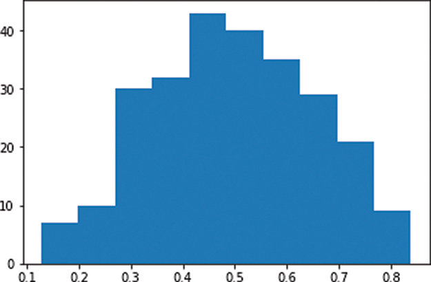
Figure 9.2 Histogram of the a activations output by a layer of sigmoid neurons, with weights initialized using the Glorot normal distribution
7. Select Kernel from the Jupyter notebook menu bar and choose Restart & Run All. This ensures you start completely fresh and don’t reuse old parameters from the previous run.
In stark contrast to Figure 9.1, the a activations obtained from our layer of sigmoid neurons is now normally distributed with a mean of ~0.5 and few (if any) values at the extremes of the sigmoid range (i.e., less than 0.1 or greater than 0.9). This is a good starting point for a neural network because now:
Few, if any, of the neurons are saturated.
It implies that the neurons generally have weak opinions about how x would influence y, which—prior to any training on data—is sensible.
![]()
In addition to the Glorot normal distribution, there is also the Glorot uniform distribution.8 The impact of selecting one of these Glorot distributions over the other when initializing your model weights is generally unnoticeable. You’re welcome to rerun the notebook while sampling values from the Glorot uniform distribution by setting w_init equal to glorot_uniform(). Your histogram of activations should come out more or less indistinguishable from Figure 9.2.
8. The Glorot uniform distribution is on the range [l; l] where .
By swapping out the sigmoid activation function in Example 9.2 with tanh (Activation('tanh')) or ReLU (Activation('relu')) in the Weight Initialization notebook, you can observe the consequences of initializing weights with values sampled from a standard normal distribution relative to a Glorot distribution across a range of activations. As shown in Figure 9.3, regardless of the chosen activation function, weight initialization with the standard normal leads to a activation outputs that are extreme relative to those obtained when initializing with Glorot.
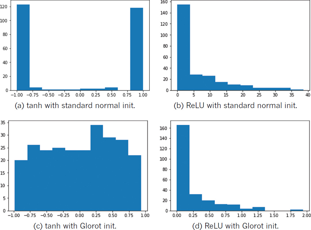
Figure 9.3 The activations output by a dense layer of 256 neurons, while varying activation function (tanh or ReLU) and weight initialization (standard normal or Glorot uniform). Note that while the distributions in (b) and (d) appear comparable at first glance, the standard normal initialization produced large activation values (reaching toward 40) while all the activations resulting from Glorot initialization are below 2.
To be sure you’re aware of the parameter initialization approach used by Keras, you can delve into the library’s documentation on a layer-by-layer basis, but, as we’ve suggested here, its default configuration is typically to initialize biases with 0 and to initialize weights with a Glorot distribution.
![]()
9. He, Y., et al. (2015). Delving deep into rectifiers: Surpassing human-level performance on ImageNet classification. arXiv: 1502.01852.
10. LeCun, Y., et al. (1998). Efficient backprop. In G. Montavon et al. (Eds.) Neural Networks: Tricks of the Trade. Lecture Notes in Computer Science, 7700 (pp. 355–65). Berlin: Springer.
Unstable Gradients
Another issue associated with artificial neural networks, and one that becomes especially perturbing as we add more hidden layers, is unstable gradients. Unstable gradients can either be vanishing or explosive in nature. We cover both varieties in turn here, and then discuss a solution to these issues called batch normalization.
Vanishing Gradients
Recall that using the cost C between the network’s predicted ŷ and the true y, as depicted in Figure 8.6, backpropagation works its way from the output layer toward the input layer, adjusting network parameters with the aim of minimizing cost. As exemplified by the mountaineering trilobite in Figure 8.2, each of the parameters is adjusted in proportion to its gradient with respect to cost: If, for example, the gradient of a parameter (with respect to the cost) is large and positive, this implies that the parameter contributes a large amount to the cost, and so decreasing it proportionally would correspond to a decrease in cost.11
11. The change is directly proportional to the negative magnitude of the gradient, scaled by the learning rate η.
In the hidden layer that is closest to the output layer, the relationship between its parameters and cost is the most direct. The farther away a hidden layer is from the output layer, the more muddled the relationship between its parameters and cost becomes. The impact of this is that, as we move from the final hidden layer toward the first hidden layer, the gradient of a given parameter relative to cost tends to flatten; it gradually vanishes. As a result of this, and as captured by Figure 8.8, the farther a layer is from the output layer, the more slowly it tends to learn. Because of this vanishing gradient problem, if we were to naïvely add more and more hidden layers to our neural network, eventually the hidden layers farthest from the output would not be able to learn to any extent, crippling the capacity for the network as a whole to learn to approximate y given x.
Exploding Gradients
Although they occur much less frequently than vanishing gradients, certain network architectures (e.g., the recurrent nets introduced in Chapter 11) can induce exploding gradients. In this case, the gradient between a given parameter relative to cost becomes increasingly steep as we move from the final hidden layer toward the first hidden layer. As with vanishing gradients, exploding gradients can inhibit an entire neural network’s capacity to learn by saturating the neurons with extreme values.
Batch Normalization
During neural network training, the distribution of hidden parameters in a layer may gradually move around; this is known as internal covariate shift. In fact, this is sort of the point of training: We want the parameters to change in order to learn things about the underlying data. But as the distribution of the weights in a layer changes, the inputs to the next layer might be shifted away from an ideal (i.e., normal, as in Figure 9.2) distribution. Enter batch normalization (or batch norm for short).12 Batch norm takes the a activations output from the preceding layer, subtracts the batch mean, and divides by the batch standard deviation. This acts to recenter the distribution of the a values with a mean of 0 and a standard deviation of 1 (see Figure 9.4). Thus, if there are any extreme values in the preceding layer, they won’t cause exploding or vanishing gradients in the next layer. In addition, batch norm has the following positive effects:
It allows layers to learn more independently from each other, because large values in one layer won’t excessively influence the calculations in the next layer.
It allows for selection of a higher learning rate—because there are no extreme values in the normalized activations—thus enabling faster learning.
The layer outputs are normalized to the batch mean and standard deviation, and that adds a noise element (especially with smaller batch sizes), which, in turn, contributes to regularization. (Regularization is covered in the next section, but suffice it to say here that regularization helps a network generalize to data it hasn’t encountered previously, which is a good thing.)

Figure 9.4 Batch normalization transforms the distribution of the activations output by a given layer of neurons toward a standard normal distribution.
12. Ioffe, S., & Szegedy, C. (2015). Batch normalization: Accelerating deep network training by reducing internal covariate shift. arXiv: 1502.03167.
Batch normalization adds two extra learnable parameters to any given layer it is applied to: γ (gamma) and β (beta). In the final step of batch norm, the outputs are linearly transformed by multiplying by γ and adding β, where γ is analogous to the standard deviation, and β to the mean. (You may notice this is the exact inverse of the operation that normalized the output values in the first place!) However, the output values were originally normalized by the batch mean and batch standard deviation, whereas γ and β are learned by SGD. We initialize the batch norm layer with γ = 1 and β = 0, and thus at the start of training this linear transformation makes no changes; batch norm is allowed to normalize the outputs as intended. As the network learns, though, it may determine that denormalizing any given layer’s activations is optimal for reducing cost. In this way, if batch norm is not helpful the network will learn to stop using it on a layer-by-layer basis. Indeed, because γ and β are continuous variables, the network can decide to what degree it would like to denormalize the outputs, depending on what works best to minimize the cost. Pretty neat!
Model Generalization (Avoiding Overfitting)
In Chapter 8, we mention that after training a model for a certain number of epochs the cost calculated on the validation dataset—which may have been decreasing nicely over earlier epochs—could begin to increase despite the fact that the cost calculated on the training dataset is still decreasing. This situation—when training cost continues to go down while validation cost goes up—is formally known as overfitting.
We illustrate the concept of overfitting in Figure 9.5. Notice we have the same data points scattered along the x and y axes in each panel. We can imagine that there is some underlying distribution that describes these points, and we show a sampling from that distribution. Our goal is to generate a model that explains the relationship between x and y but, perhaps most importantly, one that also approximates the original distribution; in this way, the model will be able to generalize to new data points drawn from the distribution and not just model the sampling of points we already have.
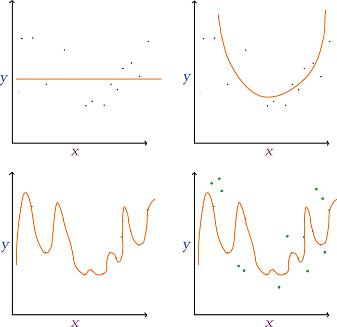
Figure 9.5 Fitting y given x using models with varying numbers of parameters. Top left: A single-parameter model underfits the data. Top right: A two-parameter model fits a parabola that suits the relationship between x and y well. Bottom left: A many-parameter model overfits the data, generalizing poorly to new data points (shown in green in the bottom-right panel).
In the first panel (top left) of Figure 9.5, we use a single-parameter model, which is limited to fitting a straight line to the data.13 This straight line underfits the data: The cost (represented by the vertical gaps between the line and the data points) is high, and the model would not generalize well to new data points. In other words, the line misses most of the points because this kind of model is not complex enough. In the next panel (top right), we use a model with two parameters, which fits a parabola-shaped curve to the data.14 With this parabolic model, the cost is much lower relative to the linear model, and it appears the model would also generalize well to new data—great!
13. This models a linear relationship, the simplest form of regression between two variables.
14. Recall the quadratic function from high school algebra.
In the third panel (bottom left) of Figure 9.5, we use a model with too many parameters—more parameters than we have data points. With this approach we reduce the cost associated with our training data points to nil: There is no perceptible gap between the curve and the data. In the last panel (bottom right), however, we show new data points from the original distribution in green, which were unseen by the model during training and so can be used to validate the model. Despite eliminating training cost entirely, the model fits these validation data poorly and so it results in a significant validation cost. The many-parameter model, dear friends, is overfit: It is a perfect model for the training data, but it doesn’t actually capture the relationship between x and y well; rather, it has learned the exact features of the training data too closely, and it subsequently performs poorly on unseen data.
Consider how in three lines of code in Example 5.6, we created a shallow neural network architecture with more than 50,000 parameters (Figure 7.5). Given this, it should not be surprising that deep learning architectures regularly have millions of parameters.15 Working with datasets that have such a large number of parameters but with perhaps only thousands of training samples could be a recipe for severe overfitting.16 Because we yearn to capitalize on deep, sophisticated network architectures even if we don’t have oodles of data at hand, thankfully we can rely on techniques specifically designed to reduce overfitting. In this section, we cover three of the best-known such techniques: L1/L2 regularization, dropout, and data augmentation.
15. Indeed, as early as Chapter 10, you’ll encounter models with tens of millions of parameters.
16. This circumstance can be annotated as n ≫ p, indicating the number of samples is much greater than the parameter count.
L1 and L2 Regularization
In branches of machine learning other than deep learning, the use of L1 or L2 regularization to reduce overfitting is prevalent. These techniques—which are alternately known as LASSO17 regression and ridge regression, respectively—both penalize models for including parameters by adding the parameters to the model’s cost function. The larger a given parameter’s size, the more that parameter adds to the cost function. Because of this, parameters are not retained by the model unless they appreciably contribute to the reduction of the difference between the model’s estimated ŷ and the true y. In other words, extraneous parameters are pared away.
17. Least absolutely shrinkage and selection operator
![]()
Dropout
L1 and L2 regularization work fine to reduce overfitting in deep learning models, but deep learning practitioners tend to favor the use of a neural-network-specific regularization technique instead. This technique, called dropout, was developed by Geoff Hinton (Figure 1.16) and his colleagues at the University of Toronto18 and was made famous by its incorporation in their benchmark-smashing AlexNet architecture (Figure 1.17).
18. Hinton, G., et al. (2012). Improving neural networks by preventing co-adaptation of feature detectors. arXiv:1207.0580.
Hinton and his coworkers’ intuitive yet powerful concept for preventing overfitting is captured by Figure 9.6. In a nutshell, dropout simply pretends that a randomly selected proportion of the neurons in each layer don’t exist during each round of training. To illustrate this, three rounds of training19 are shown in the figure. For each round, we remove a specified proportion of hidden layers by random selection. For the first hidden layer of the network, we’ve configured it to drop out one-third (33.3 percent) of the neurons. For the second hidden layer, we’ve configured 50 percent of the neurons to be dropped out. Let’s cover the three training rounds shown in Figure 9.6:
In the top panel, the second neuron of the first hidden layer and the first neuron of the second hidden layer are randomly dropped out.
In the middle panel, it is the first neuron of the first hidden layer and the second one of the second hidden layer that are selected for dropout. There is no “memory” of which neurons have been dropped out on previous training rounds, and so it is by chance alone that the neurons dropped out in the second round are distinct from those dropped out in the first.
In the bottom panel, the third neuron of the first hidden layer is dropped out for the first time. For the second consecutive round of training, the second neuron of the second hidden layer is also randomly selected.

Figure 9.6 Dropout, a technique for reducing model overfitting, involves the removal of randomly selected neurons from a network’s hidden layers in each round of training. Three rounds of training with dropout are shown here.
19. If the phrase round of training is not immediately familiar, refer to Figure 8.5 for a refresher.
Instead of reining in parameter sizes toward zero (as with batch normalization), dropout doesn’t (directly) constrain how large a given parameter value can become. Dropout is nevertheless an effective regularization technique, because it prevents any single neuron from becoming excessively influential within the network: Dropout makes it challenging for some very specific aspect of the training dataset to create an overly specific forward-propagation pathway through the network because, on any given round of training, neurons along that pathway could be removed. In this way, the model doesn’t become overreliant on certain features of the data to generate a good prediction.
When validating a neural network model that was trained using dropout, or indeed when making real-world inferences with such a network, we must take an extra step first. During validation or inference, we would like to leverage the power of the full network, that is, its total complement of neurons. The snag is that, during training, we only ever used a subset of the neurons to forward propagate x through the network and estimate ŷ. If we were to naïvely carry out this forward propagation with suddenly all of the neurons, our ŷ would emerge befuddled: There are now too many parameters, and the totals after all the mathematical operations would be larger than expected. To compensate for the additional neurons, we must correspondingly adjust our neuron parameters downward. If we had, say, dropped out half of the neurons in a hidden layer during training, then we would need to multiply the layer’s parameters by 0.5 prior to validation or inference. As a second example, for a hidden layer in which we dropped out 33.3 percent of the neurons during training, we then must multiply the layer’s parameters by 0.667 prior to validation.20 Thankfully, Keras handles this parameter-adjustment process for us automatically. When working in other deep learning libraries (e.g., low-level TensorFlow), however, you may need to be mindful and remember to carry out these adjustments yourself.
20. Put another way, if the probability of a given neuron being retained during training is p, then we multiply that neuron’s parameters by p prior to carrying out model validation or inference.
![]()
As with learning rate and mini-batch size (discussed in Chapter 8), network architecture options pertaining to dropout are hyperparameters. Here are our rules of thumb for choosing which layers to apply dropout to and how much of it to apply:
If your network is overfitting to your training data (i.e., your validation cost increases while your training cost goes down), then dropout is warranted somewhere in the network.
Even if your network isn’t obviously overfitting to your training data, adding some dropout to the network may improve validation accuracy—especially in later epochs of training.
Applying dropout to all of the hidden layers in your network may be overkill. If your network has a fair bit of depth, it may be sufficient to apply dropout solely to later layers in the network (the earliest layers may be harmlessly identifying features). To test this out, you could begin by applying dropout only to the final hidden layer and observing whether this is sufficient for curtailing overfitting; if not, add dropout to the next deepest layer, test it, and so on.
If your network is struggling to reduce validation cost or to recapitulate low validation costs attained when less dropout was applied, then you’ve added too much dropout—pare it back! As with other hyperparameters, there is a Goldilocks zone for dropout, too.
With respect to how much dropout to apply to a given layer, each network behaves uniquely and so some experimentation is required. In our experience, dropping out 20 percent up to 50 percent of the hidden-layer neurons in machine vision applications tends to provide the highest validation accuracies. In natural language applications, where individual words and phrases can convey particular significance, we have found that dropping out a smaller proportion—between 20 percent and 30 percent of the neurons in a given hidden layer—tends to be optimal.
Data Augmentation
In addition to regularizing your model’s parameters to reduce overfitting, another approach is to increase the size of your training dataset. If it is possible to inexpensively collect additional high-quality training data for the particular modeling problem you’re working on, then you should do so! The more data provided to a model during training, the better the model will be able to generalize to unseen validation data.
In many cases, collecting fresh data is a pipe dream. It may nevertheless be possible to generate new training data from existing data by augmenting it, thereby artificially expanding your training dataset. With the MNIST digits, for example, many different types of transforms would yield training samples that constitute suitable handwritten digits, such as:
Skewing the image
Blurring the image
Shifting the image a few pixels
Applying random noise to the image
Rotating the image slightly
Indeed, as shown on the personal website of Yann LeCun (see Figure 1.9 for a portrait), many of the record-setting MNIST validation dataset classifiers took advantage of such artificial training dataset expansion.21,22
22. We will use Keras data-augmentation tools on actual images of hot dogs in Chapter 10.
Fancy Optimizers
So far in this book we’ve used only one optimization algorithm: stochastic gradient descent. Although SGD performs well, researchers have devised shrewd ways to improve it.
Momentum
The first SGD improvement is to consider momentum. Here’s an analogy of the principle: Let’s imagine it’s winter and our intrepid trilobite is skiing down a snowy gradient-mountain. If a local minimum is encountered (as in the middle panel of Figure 8.7), the momentum of the trilobite’s movement down the slippery hill will keep it moving, and the minimum will be easily bypassed. In this way, the gradients on previous steps have influenced the current step.
We calculate momentum in SGD by taking a moving average of the gradients for each parameter and using that to update the weights in each step. When using momentum, we have the additional hyperparameter β (beta), which ranges from 0 to 1, and which controls how many previous gradients are incorporated in the moving average. Small β values permit older gradients to contribute to the moving average, something that can be unhelpful; the trilobite wouldn’t want the steepest part of the hill to guide its speed as it approaches the lodge for its après-ski drinks. Typically we’d use larger β values, with β = 0.9 serving as a reasonable default.
Nesterov Momentum
Another version of momentum is called Nesterov momentum. In this approach, the moving average of the gradients is first used to update the weights and find the gradients at whatever that position may be; this is equivalent to a quick peek at the position where momentum might take us. We then use the gradients from this sneak-peek position to execute a gradient step from our original position. In other words, our trilobite is suddenly aware of its speed down the hill, so it’s taking that into account, guessing where its own momentum might be taking it, and then adjusting its course before it even gets there.
AdaGrad
Although both momentum approaches improve SGD, a shortcoming is that they both use a single learning rate η for all parameters. Imagine, if you will, that we could have an individual learning rate for each parameter, thus enabling those parameters that have already reached their optimum to slow or halt learning, while those that are far from their optima can keep going. Well, you’re in luck! That’s exactly what can be achieved with the other optimizers we’ll discuss in this section: AdaGrad, AdaDelta, RMSProp, and Adam.
The name AdaGrad comes from “adaptive gradient.”23 In this variation, every parameter has a unique learning rate that scales depending on the importance of that feature. This is especially useful for sparse data where some features occur only rarely: When those features do occur, we’d like to make larger updates of their parameters. We achieve this individualization by maintaining a matrix of the sum of squares of the past gradients for each parameter, and dividing the learning rate by its square root. AdaGrad is the first introduction to the parameter ∊ (epsilon), which is a doozy: Epsilon is a smoothing factor to avoid divide-by-zero errors and can safely be left at its default value of ∊ = 1 × 10–8.24
23. Duchi, J., et al. (2011). Adaptive subgradient methods for online learning and stochastic optimization. Journal of Machine Learning Research, 12, 2121–59.
24. AdaGrad, AdaDelta, RMSProp, and Adam all use∊ for the same purpose, and it can be left at its default across all of these methods.
A significant benefit of AdaGrad is that it minimizes the need to tinker with the learning rate hyperparameter η. You can generally just set-it-and-forget-it at its default of η = 0.01. A considerable downside of AdaGrad is that, as the matrix of past gradients increases in size, the learning rate is increasingly divided by a larger and larger value, which eventually renders the learning rate impractically small and so learning essentially stops.
AdaDelta and RMSProp
AdaDelta resolves the gradient-matrix-size shortcoming of AdaGrad by maintaining a moving average of previous gradients in the same manner that momentum does.25 AdaDelta also eliminates the η term, so a learning rate doesn’t need to be configured at all.26
25. Zeiler, M.D. (2012). ADADELTA: An adaptive learning rate method. arXiv:1212.5701.
26. This is achieved through a crafty mathematical trick that we don’t think is worth expounding on here. You may notice, however, that Keras and TensorFlow still have a learning rate parameter in their implementations of AdaDelta. In those cases, it is recommended to leave η at 1, that is, no scaling and therefore no functional learning rate as you have come to know it in this book.
RMSProp (root mean square propagation) was developed by Geoff Hinton (see Figure 1.16 for a portrait) at about the same time as AdaDelta.27 It works similarly except it retains the learning rate η parameter. Both RMSProp and AdaDelta involve an extra hyperparameter ρ (rho), or decay rate, which is analogous to the β value from momentum and which guides the size of the window for the moving average. Recommended values for the hyperparameters are ρ = 0.95 for both optimizers, and setting η = 0.001 for RMSProp.
27. This optimizer remains unpublished. It was first proposed in Lecture 6e of Hinton’s Coursera Course “Neural Networks for Machine Learning” (www.cs.toronto.edu/∼hinton/coursera/lecture6/lec6.pdf).
Adam
The final optimizer we discuss in this section is also the one we employ most often in the book. Adam—short for adaptive moment estimation—builds on the optimizers that came before it.28 It’s essentially the RMSProp algorithm with two exceptions:
An extra moving average is calculated, this time of past gradients for each parameter (called the average first moment of the gradient,29 or simply the mean) and this is used to inform the update instead of the actual gradients at that point.
A clever bias trick is used to help prevent these moving averages from skewing toward zero at the start of training.
28. Kingma, D.P., & Ba, J. (2014). Adam: A method for stochastic optimization. arXiv:1412.6980.
29. The other moving average is of the squares of the gradient, which is the second moment of the gradient, or the variance.
Adam has two β hyperparameters, one for each of the moving averages that are calculated. Recommended defaults are β1 = 0.9 and β2 = 0.999. The learning rate default with Adam is η = 0.001, and you can generally leave it there.
Because RMSProp, AdaDelta, and Adam are so similar, they can be used interchangeably in similar applications, although the bias correction may help Adam later in training. Even though these newfangled optimizers are in vogue, there is still a strong case for simple SGD with momentum (or Nesterov momentum), which in some cases performs better. As with other aspects of deep learning models, you can experiment with optimizers and observe what works best for your particular model architecture and problem.
A Deep Neural Network in Keras
We can now sound the trumpet, because we’re reached a momentous milestone! With the additional theory we’ve covered in this chapter, you have enough knowledge under your belt to competently design and train a deep learning model. If you’d like to follow along interactively as we do so, pop into the accompanying Deep Net in Keras Jupyter notebook. Relative to our shallow and intermediate-depth model notebooks (refer to Example 5.1), we have a pair of additional dependencies—namely, dropout and batch normalization—as provided in Example 9.4.
Example 9.4 Additional dependencies for deep net in Keras
from keras.layers import Dropout
from keras.layers.normalization import BatchNormalization
We load and preprocess the MNIST data in the same way as previously. As shown in Example 9.5, it’s the neural network architecture cell where we begin to diverge.
Example 9.5 Deep net in Keras model architecture
model = Sequential()

model.add(Dense(64, activation='relu', input_shape=(784,)))
model.add(BatchNormalization())

model.add(Dense(64, activation='relu'))
model.add(BatchNormalization())

model.add(Dense(64, activation='relu'))
model.add(BatchNormalization())
model.add(Dropout(0.2))

model.add(Dense(10, activation='softmax'))
As before, we instantiate a Sequential model object. After we add our first hidden layer to it, however, we also add a BatchNormalization() layer. In doing this we are not adding an actual layer replete with neurons, but rather we’re adding the batch-norm transformation for the activations a from the layer before (the first hidden layer). As with the first hidden layer, we also add a BatchNormalization() layer atop the second hidden layer of neurons. Our output layer is identical to the one used in the shallow and intermediate-depth nets, but to create an honest-to-goodness deep neural network, we are further adding a third hidden layer of neurons. As with the preceding hidden layers, the third hidden layer consists of 64 batch-normalized relu neurons. We are, however, supplementing this final hidden layer with Dropout, set to remove one-fifth (0.2) of the layer’s neurons during each round of training.
As captured in Example 9.6, the only other change relative to our intermediate-depth network is that we use the Adam optimizer (optimizer='adam') in place of ordinary SGD optimization.
Example 9.6 Deep net in Keras model compilation
model.compile(loss='categorical_crossentropy',
              optimizer='adam',
              metrics=['accuracy'])
Note that we need not supply any hyperparameters to the Adam optimizer, because Keras automatically includes all the sensible defaults we detailed in the preceding section. For all of the other optimizers we covered, Keras (and TensorFlow, for that matter) has implementations that can easily be dropped in in place of ordinary SGD or Adam. You can refer to the documentation for those libraries online to see exactly how it’s done.
When we call the fit() method on our model,30 we discover that our digestion of all the additional theory in this chapter paid off: With our intermediate-depth network, our validation accuracy plateaued around 97.6 percent, but our deep net attained 97.87 percent validation accuracy following 15 epochs of training (see Figure 9.7), shaving away 11 percent of our already-small error rate. To squeeze even more juice out of the error-rate lemon than that, we’re going to need machine-vision-specific neuron layers such as those introduced in the upcoming Chapter 10.
![Epoch 15/20 60000/60000 [========================] - 1s 23us/step loss: 0.0288 acc: 0.9906 val_loss: 0.0865 val_acc: 0.9787 Epoch 16/20 60000/60000 [========================]- 22us/step loss: 0.0246 acc: 0.9919 val_loss: 0.0880 val_acc: 0.9767](http://images-20200215.ebookreading.net/5/4/4/9780135116821/9780135116821__deep-learning-illustrated__9780135116821__graphics__krohn_f09_07.jpg)
Figure 9.7 Our deep neural network architecture peaked at a 97.87 percent validation following 15 epochs of training, besting the accuracy of our shallow and intermediate-depth architectures. Because of the randomness of network initialization and training, you may obtain a slightly lower or a slightly higher accuracy with the identical architecture.
30. This model.fit() step is exactly the same as for our Intermediate Net in Keras notebook, that is, Example 8.3.
Regression
In Chapter 4, when discussing supervised learning problems, we mentioned that these can involve either classification or regression. In this book, nearly all our models are used for classifying inputs into one category or another. In this section, however, we depart from that tendency and highlight how to adapt neural network models to regression tasks—that is, any problem where you’d like to predict some continuous variable. Examples of regression problems include predicting the future price of a stock, forecasting how many centimeters of rain may fall tomorrow, and modeling how many sales to expect of a particular product. In this section, we use a neural network and a classic dataset to estimate the price of housing near Boston, Massachusetts, in the 1970s.
Our dependencies, as shown in our Regression in Keras notebook, are provided in Example 9.7. The only unfamiliar dependency is the boston_housing dataset, which is conveniently bundled into the Keras library.
Example 9.7 Regression model dependencies
from keras.datasets import boston_housing
from keras.models import Sequential
from keras.layers import Dense, Dropout
from keras.layers.normalization import BatchNormalization
Loading the data is as simple as with the MNIST digits:
(X_train, y_train), (X_valid, y_valid) = boston_housing.load_data()
Calling the shape parameter of X_train and X_valid, we find that there are 404 training cases and 102 validation cases. For each case—a distinct area of the Boston suburbs—we have 13 predictor variables related to building age, mean number of rooms, crime rate, the local student-to-teacher ratio, and so on.31 The median house price (in thousands of dollars) for each area is provided in the y variables. As an example, the first case in the training set has a median house price of $15,200.32
31. You can read more about the data by referring to the article they were originally published in: Harrison, D., & Rubinfeld, D. L. (1978). Hedonic prices and the demand for clean air. Journal of Environmental Economics and Management, 5, 81–102.
32. Running y_train[0] returns 15.2.
The network architecture we built for house-price prediction is provided in Example 9.8.
Example 9.8 Regression model network architecture
model = Sequential()

model.add(Dense(32, input_dim=13, activation='relu'))
model.add(BatchNormalization())

model.add(Dense(16, activation='relu'))
model.add(BatchNormalization())
model.add(Dropout(0.2))

model.add(Dense(1, activation='linear'))
Reasoning that with only 13 input values and a few hundred training cases we would gain little from a deep neural network with oodles of neurons in each layer, we opted for a two-hidden-layer architecture consisting of merely 32 and 16 neurons per layer. We applied batch normalization and a touch of dropout to avoid overfitting to the particular cases of the training dataset. Most critically, in the output layer we set the activation argument to linear—the option to go with when you’d like to predict a continuous variable, as we do when performing regression. The linear activation function outputs z directly so that the network’s ŷ can be any numeric value (representing, e.g., dollars, centimeters) instead of being squashed into a probability between 0 and 1 (as happens when you use the sigmoid or softmax activation functions).
When compiling the model (see Example 9.9), another regression-specific adjustment we made is using mean squared error (MSE) in place of cross-entropy (loss='mean_squared_error'). While we’ve used cross-entropy cost exclusively so far in this book, that cost function is specifically designed for classification problems, in which ŷ is a probability. For regression problems, where the output is inherently not a probabilty, we use MSE instead.33
33. There are other cost functions applicable to regression problems, such as mean absolute error (MAE) and Huber loss, although these aren’t covered in this book. MSE should serve you well enough.
Example 9.9 Compiling a regression model
model.compile(loss='mean_squared_error', optimizer='adam')
You may have noticed that we left out the accuracy metric when compiling this time around. This is deliberate: There’s no point in calculating accuracy, because this metric (the percentage of cases classified correctly) isn’t relevant to continuous variables as it is with categorical ones.34
34. It’s also helpful to remember that, generally, accuracy is used only to set our minds at ease about how well our models are performing. The model itself learns from the cost, not the accuracy.
Fitting our model (as in Example 9.10) is one step that is no different from classification.
Example 9.10 Fitting a regression model
model.fit(X_train, y_train,
          batch_size=8, epochs=32, verbose=1,
          validation_data=(X_valid, y_valid))
We trained for 32 epochs because, in our experience with this particular model, training for longer produced no lower validation losses. We didn’t spend any time optimizing the batch-size hyperparameter, so there could be small accuracy gains to be made by varying it.
During our particular run of the regression model, our lowest validation loss (25.7) was attained in the 22nd epoch. By our final (32nd) epoch, this loss had risen considerably to 56.5 (for comparison, we had a validation loss of 56.6 after just one epoch). In Chapter 11, we demonstrate how to save your model parameters after each epoch of training so that the best-performing epoch can be reloaded later, but for the time being we’re stuck with the relatively crummy parameters from the final epoch. In any event, if you’d like to see specific examples of model house-price inferences given some particular input data, you can do this by running the code provided in Example 9.11.35
35. Note that we had to use the NumPy reshape method to pass in the 13 predictor variables of the 43rd case as a row-oriented array of values ([1, 13]) as opposed to as a column.
Example 9.11 Predicting the median house price in a particular suburb of Boston
model.predict(np.reshape(X_valid[42], [1, 13]))
This returned for us a predicted median house price (ŷ) of $20,880 for the 43rd Boston suburb in the validation dataset. The actual median price (y; which can be output by calling y_valid[42]) is $14,100.
TensorBoard
When evaluating the performance of your model epoch over epoch, it can be tedious and time-consuming to read individual results numerically, as we did after running the code in Example 9.10, particularly if the model has been training for many epochs. Instead, TensorBoard (Figure 9.8) is a convenient, graphical tool for:
Visually tracking model performance in real time
Reviewing historical model performances
Comparing the performance of various model architectures and hyperparameter settings applied to fitting the same data
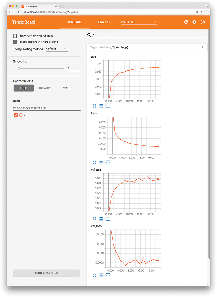
Figure 9.8 The TensorBoard dashboard enables you to, epoch over epoch, visually track your model’s cost (loss) and accuracy (acc) across both your training data and your validation (val) data.
TensorBoard comes automatically with the TensorFlow library, and instructions for getting it up and running are available via the TensorFlow site.36 It’s generally straightforward to set up. Provided here, for example, is a procedure that adapts our Deep Net in Keras notebook for TensorBoard use on a Unix-based operating system, including macOS:
36. tensorflow.org/guide/summaries_and_tensorboard
As shown in Example 9.12, change your Python code as follows:37
37. This is also laid out in our Deep Net in Keras with TensorBoard notebook.
Import the
TensorBoarddependency fromkeras.callbacks.Instantiate a TensorBoard object (we’ll call it
tensorboard), and specify a new, unique directory name (e.g.,deep-net) that you’d like to create and have TensorBoard log data written into for this particular run of model-fitting:tensorboard = TensorBoard(log_dir='logs/deep-net')
Pass the TensorBoard object as a
callbackparameter to thefit()method:callbacks = [tensorboard]
In your terminal, run the following:38
38. Note: We specified the same logging directory location that the TensorBoard object was set to use in step 1b. Since we specified a relative path and not an absolute path for our logging directory, we need to be mindful to run the tensorboard command from the same directory as our Deep Net in Keras with TensorBoard notebook.
tensorboard --logdir='logs/deep-net' --port 6006
Navigate to
localhost:6006in your favorite web browser.
Example 9.12 Using TensorBoard while fitting a model in Keras
from keras.callbacks import TensorBoard
tensorboard = TensorBoard('logs/deep-net')
model.fit(X_train, y_train,
          batch_size=128, epochs=20,
          verbose=1,
          validation_data=(X_valid, y_valid),
          callbacks=[tensorboard])
By following these steps or an analogous procedure for the circumstances of your particular operating system, you should see something like Figure 9.8 in your browser window. From there, you can visually track any given model’s cost and accuracy across both your training and validation datasets in real time as these metrics change epoch over epoch. This kind of performance tracking is one of the primary uses of TensorBoard, although the dashboard interface also provides heaps of other functionality, such as visual breakdowns of your neural network graph and the distribution of your model weights. You can learn about these additional features by reading the TensorBoard docs and exploring the interface on your own.
Summary
Over the course of the chapter, we discussed common pitfalls in modeling with neural networks and covered strategies for minimizing their impact on model performance. We wrapped up the chapter by applying all of the theory learned thus far in the book to construct our first bona fide deep learning network, which provided us with our best-yet accuracy on MNIST handwritten-digit classification. While such deep, dense neural nets are applicable to generally approximating any given output y when provided some input x, they may not be the most efficient option for specialized modeling. Coming up next in Part III, we introduce neural network layers and deep learning approaches that excel at particular, specialized tasks, including machine vision, natural language processing, the generation of art, and playing games.
Key Concepts
Here are the essential foundational concepts thus far. New terms from the current chapter are highlighted in purple.
parameters:
weight w
bias b
activation a
artificial neurons:
sigmoid
tanh
ReLU
linear
input layer
hidden layer
output layer
layer types:
dense (fully connected)
softmax
cost (loss) functions:
quadratic (mean squared error)
cross-entropy
forward propagation
backpropagation
unstable (especially vanishing) gradients
Glorot weight initialization
batch normalization
dropout
optimizers:
stochastic gradient descent
Adam
optimizer hyperparameters:
learning rate η
batch size