10
Data Frames
This chapter introduces data frame values, which are the primary two-dimensional data storage type used in R. In many ways, data frames are similar to the row-and-column table layout that you may be familiar with from spreadsheet programs like Microsoft Excel. Rather than interact with this data structure through a user interface (UI), you will learn how to programmatically and reproducibly perform operations on this data type. This chapter covers ways of creating, describing, and accessing data from data frames in R.
10.1 What Is a Data Frame?
At a practical level, data frames act like tables, where data is organized into rows and columns. For example, reconsider the table of names, weights, and heights from Chapter 9, shown in Figure 10.1. In R, you can use data frames to represent these kinds of tables.

Data frames are really just lists (see Chapter 8) in which each element is a vector of the same length. Each vector represents a column, not a row. The elements at corresponding indices in the vectors are considered part of the same row (record). This structure makes sense because each row may have different types of data—such as a person’s name (string) and height (number)—and vector elements must all be of the same type.
For example, you can think of the data shown in Figure 10.1 as a list of three vectors: name, height, and weight. The name, height, and weight of the first person measured are represented by the first elements of the name, height, and weight vectors, respectively.
You can work with data frames as if they were lists, but data frames have additional properties that make them particularly well suited for handling tables of data.
10.2 Working with Data Frames
Many data science questions can be answered by honing in on the desired subset of your data. In this section, you will learn how to create, describe, and access data from data frames.
10.2.1 Creating Data Frames
Typically you will load data sets from some external source (see Section 10.3), rather than writing out the data by hand. However, it is also possible to construct a data frame by combining multiple vectors. To accomplish this, you can use the data.frame() function, which accepts vectors as arguments, and creates a table with a column for each vector. For example:
# Create a data frame by passing vectors to the `data.frame()` function

# A vector of names
name <- c("Ada", "Bob", "Chris", "Diya", "Emma")

# A vector of heights
height <- c(64, 74, 69, 69, 71)

# A vector of weights
weight <- c(135, 156, 139, 144, 152)

# Combine the vectors into a data frame
# Note the names of the variables become the names of the columns!
people <- data.frame(name, height, weight, stringsAsFactors = FALSE)
The last argument to the data.frame() function is included because one of the vectors contains strings; it tells R to treat that vector as a typical vector, instead of another data type called a factor when constructing the data frame. This is usually what you will want to do—see Section 10.3.2 for more information.
You can also specify data frame column names using the key = value syntax used by named lists when you create your data frame:
# Create a data frame of names, weights, and heights,
# specifying column names to use
people <- data.frame(
  name = c("Ada", "Bob", "Chris", "Diya", "Emma"),
  height = c(64, 74, 69, 69, 71),
  weight = c(135, 156, 139, 144, 152)
)
Because data frame elements are lists, you can access the values from people using the same dollar notation and double-bracket notation as you use with lists:
# Retrieve information from a data frame using list-like syntax

# Create the same data frame as above
people <- data.frame(name, height, weight, stringsAsFactors = FALSE)

# Retrieve the `weight` column (as a list element); returns a vector
people_weights <- people$weight

# Retrieve the `height` column (as a list element); returns a vector
people_heights <- people[["height"]]
For more flexible approaches to accessing data from data frames, see section 10.2.3.
10.2.2 Describing the Structure of Data Frames
While you can interact with data frames as lists, they also offer a number of additional capabilities and functions. For example, Table 10.1 presents a few functions you can use to inspect the structure and content of a data frame:
Table 10.1 Functions for inspecting data frames
Function |
Description |
|
Returns the number of rows in the data frame |
|
Returns the number of columns in the data frame |
|
Returns the dimensions (rows, columns) in the data frame |
|
Returns the names of the columns of the data frame |
|
Returns the names of the rows of the data frame |
|
Returns the first few rows of the data frame (as a new data frame) |
|
Returns the last few rows of the data frame (as a new data frame) |
|
Opens the data frame in a spreadsheet-like viewer (only in RStudio) |
# Use functions to describe the shape and structure of a data frame

# Create the same data frame as above
people <- data.frame(name, height, weight, stringsAsFactors = F)

# Describe the structure of the data frame
nrow(people) # [1] 5
ncol(people) # [1] 3
dim(people) # [1] 5 3
colnames(people) # [1] "name" "height" "weight"
rownames(people) # [1] "1" "2" "3" "4" "5"

# Create a vector of new column names
new_col_names <- c("first_name", "how_tall", "how_heavy")

# Assign that vector to be the vector of column names
colnames(people) <- new_col_names
Many of these description functions can also be used to modify the structure of a data frame. For example, you can use the colnames() functions to assign a new set of column names to a data frame.
10.2.3 Accessing Data Frames
As stated earlier, since data frames are lists, it’s possible to use dollar notation (my_df$column_name) or double-bracket notation (my_df[["column_name"]]) to access entire columns. However, R also uses a variation of single-bracket notation that allows you to filter for and access individual data elements (cells) in the table. In this syntax, you put two values separated by a comma (,) inside of single square brackets—the first argument specifies which row(s) you want to extract, while the second argument specifies which column(s) you want to extract.
Table 10.2 summarizes how single-bracket notation can be used to access data frames. Take special note of the fourth option’s syntax (for retrieving rows): you still include the comma (,), but because you leave the which column value blank, you get all of the columns!
Table 10.2 Accessing a data frame with single bracket notation
Syntax |
Description |
Example |
|
Element(s) by row and column names |
(element in row named |
|
Element(s) by row and column indices |
(element in the second row, third column) |
|
Element(s) by row and column; can mix names and indices |
(second element in the |
|
All elements (columns) in row name or index |
(all columns in the second row) |
|
All elements (rows) in a column name or index |
(all rows in the |
# Assign a set of row names for the vector
# (using the values in the `name` column)
rownames(people) <- people$name

# Extract the row with the name "Ada" (and all columns)
people["Ada", ] # note the comma, indicating all columns

# Extract the second column as a vector
people[, "height"] # note the comma, indicating all rows

# Extract the second column as a data frame (filtering)
people["height"] # without a comma, it returns a data frame
Of course, because numbers and strings are stored in vectors, you’re actually specifying vectors of names or indices to extract. This allows you to get multiple rows or columns:
# Get the `height` and `weight` columns
people[, c("height", "weight")] # note the comma, indicating all rows

# Get the second through fourth rows
people[2:4, ] # note the comma, indicating all columns
Additionally, you can use a vector of boolean values to specify your indices of interest (just as you did with vectors):
# Get rows where `people$height` is greater than 70 (and all columns)
people[people$height > 70, ] # rows for which `height` is greater than 70
Remember
The type of data that is returned when selecting data using single brackets depends on how many columns you are selecting. Extracting values from more than one column will produce a data frame; extracting from just one column will produce a vector.
Tip
In general, it’s easier, cleaner, and less buggy to filter by column name (character string), rather than by column number, because it’s not unusual for column order to change in a data frame. You should almost never access data in a data frame by its positional index. Instead, you should use the column name to specify columns, and a filter to specify rows of interest.
Going Further
10.3 Working with CSV Data
Section 10.2 demonstrated constructing your own data frames by “hard-coding” the data values. However, it is much more common to load data from somewhere else, such as a separate file on your computer or a data resource on the internet. R is also able to ingest data from a variety of sources. This section focuses on reading tabular data in comma-separated value (CSV) format, usually stored in a file with the extension .csv. In this format, each line of the file represents a record (row) of data, while each feature (column) of that record is separated by a comma:
name, weight, height
Ada, 64, 135
Bob, 74, 156
Chris, 69, 139
Diya, 69, 144
Emma, 71, 152
Most spreadsheet programs, such as Microsoft Excel, Numbers, and Google Sheets, are just interfaces for formatting and interacting with data that is saved in this format. These programs easily import and export .csv files. But note that .csv files are unable to save the formatting and calculation formulas used in those programs—a .csv file stores only the data!
You can load the data from a .csv file into R by using the read.csv() function:
# Read data from the file `my_file.csv` into a data frame `my_df`
my_df <- read.csv("my_file.csv", stringsAsFactors = FALSE)
Again, use the stringsAsFactors argument to make sure string data is stored as a vector rather than as a factor (see Section 10.3.2 for details). This function will return a data frame just as if you had created it yourself.
Remember
If an element is missing from a data frame (which is very common with real-world data), R will fill that cell with the logical value NA, meaning “not available.” There are multiple waysa to handle this in an analysis; you can filter for those values using bracket notation to replace them, exclude them from your analysis, or impute them using more sophisticated techniques.
aSee, for example, http://www.statmethods.net/input/missingdata.html
Conversely, you can write data to a .csv file using the write.csv() function, in which you specify the data frame you want to write, the filename of the file you want to write the data to, and other optional arguments:
# Write the data in `my_df` to the file `my_new_file.csv`
# The `row.names` argument indicates if the row names should be
# written to the file (usually not)
write.csv(my_df, "my_new_file.csv", row.names = FALSE)
Additionally, there are many data sets you can explore that ship with the R software. You can see a list of these data sets using the data() function, and begin working with them directly (try View(mtcars) as an example). Moreover, many packages include data sets that are well suited for demonstrating their functionality. For a robust (though incomplete) list of more than 1,000 data sets that ship with R packages, see this webpage.1
1R Package Data Sets: https://vincentarelbundock.github.io/Rdatasets/datasets.html
10.3.1 Working Directory
The biggest complication when working with .csv files is that the read.csv() function takes as an argument a path to a file. Because you want this script to work on any computer (to support collaboration, or so you can code from your personal computer or a computer at a library), you need to be sure to use a relative path to the file. The question is: relative to what?
Like the command line, the R interpreter (running inside RStudio) has a current working directory from which all file paths are relative. The trick is that the working directory is not necessarily the directory of the current script file! This makes sense, as you may have many files open in RStudio at the same time, and your R interpreter can have only one working directory.
Just as you can view the current working directory when on the command line (using pwd), you can use an R function to view the current working directory when in R:
# Get the absolute path to the current working directory
getwd() # returns a path like /Users/YOUR_NAME/Documents/projects
You often will want to change the working directory to be your project’s directory (wherever your scripts and data files happen to be; often the root of your project repository). It is possible to change the current working directory using the setwd() function. However, this function also takes an absolute path, so doesn’t fix the problem of working across machines. You should not include this absolute path in your script (though you could use it from the console).
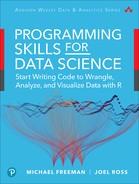
A better solution is to use RStudio itself to change the working directory. This is reasonable because the working directory is a property of the current running environment, which is what RStudio makes accessible. The easiest way to do this is to use the Session > Set Working Directory menu option (see Figure 10.2): you can either set the working directory To Source File Location (the folder containing whichever .R script you are currently editing; this is usually what you want), or you can browse for a particular directory with Choose Directory.
Session > Set Working Directory to change the working directory through RStudio.As a specific example, consider trying to load the my-data.csv file from the analysis.R script, given the folder structure illustrated in Figure 10.3. In your analysis.R script you want to be able to use a relative path to access your data (my-data.csv). In other words, you don’t want to have to specify the absolute path (/Users/YOUR_NAME/Documents/projects/analysis-project/ data/my-data.csv) to find this. Instead, you want to provide instructions on how your program can find your data file relative to where you are working (in your analysis.R file). After setting the session’s path to the working directory, you will be able to use the relative path to find it:
# Load the data using a relative path
# (this works only after setting the working directory,
# most easily with the RStudio UI)
my_data <- read.csv("data/my-data.csv", stringsAsFactors = FALSE)

my-data.csv file from the analysis.R script using the relative path data/my-data.csv.10.3.2 Factor Variables
Remember
You should always include a stringsAsFactors = FALSE argument when either loading or creating data frames. This section explains why you need to do that.
Factors are a data structure for optimizing variables that consist of a finite set of categories (i.e., they are categorical variables). For example, imagine that you had a vector of shirt sizes that could take on only the values small, medium, or large. If you were working with a large data set (thousands of shirts!), it would end up taking up a lot of memory to store the character strings (5+ letters per word at 1 or more bytes per letter) for each of those variables.
A factor would instead store a number (called a level) for each of these character strings—for example, 1 for small, 2 for medium, or 3 for large (though the order of the numbers may vary). R will remember the relationship between the integers and their labels (the strings). Since each number takes just 2–4 bytes (rather than 1 byte per letter), factors allow R to keep much more information in memory.
To see how factor variables appear similar to (but are actually different from) vectors, you can create a factor variable using as.factor():
# Demonstrate the creation of a factor variable

# Start with a character vector of shirt sizes
shirt_sizes <- c("small", "medium", "small", "large", "medium", "large")

# Create a factor representation of the vector
shirt_sizes_factor <- as.factor(shirt_sizes)

# View the factor and its levels
print(shirt_sizes_factor)
# [1] small  medium small  large  medium large
# Levels: large medium small

# The length of the factor is still the length of the vector,
# not the number of levels
length(shirt_sizes_factor) # 6
When you print out the shirt_sizes_factor variable, R still (intelligently) prints out the labels that you are presumably interested in. It also indicates the levels, which are the only possible values that elements can take on.
It is worth restating: factors are not vectors. This means that most all the operations and functions you want to use on vectors will not work:
# Attempt to apply vector methods to factors variables: it doesn't work!

# Create a factor of numbers (factors need not be strings)
num_factors <- as.factor(c(10, 10, 20, 20, 30, 30, 40, 40))

# Print the factor to see its levels
print(num_factors)
# [1] 10 10 20 20 30 30 40 40
# Levels: 10 20 30 40

# Multiply the numbers by 2
num_factors * 2 # Warning Message: '*' not meaningful for factors
# Returns vector of NA instead

# Changing entry to a level is fine
num_factors[1] <- 40

# Change entry to a value that ISN'T a level fails
num_factors[1] <- 50 # Warning Message: invalid factor level, NA generated
# num_factors[1] is now NA
If you create a data frame with a string vector as a column (as happens with read.csv()), it will automatically be treated as a factor unless you explicitly tell it not to be:
# Attempt to replace a factor with a (new) string: it doesn't work!

# Create a vector of shirt sizes
shirt_size <- c("small", "medium", "small", "large", "medium", "large")

# Create a vector of costs (in dollars)
cost <- c(15.5, 17, 17, 14, 12, 23)

# Data frame of inventory (by default, stringsAsFactors is set to TRUE)
shirts_factor <- data.frame(shirt_size, cost)

# Confirm that the `shirt_size` column is a factor
is.factor(shirts_factor$shirt_size) # TRUE

# Therefore, you are unable to add a new size like "extra-large"
shirts_factor[1, 1] <- "extra-large"
# Warning: invalid factor level, NA generated
The NA produced in the preceding example can be avoided if the stringsAsFactors option is set to FALSE:
# Avoid the creation of factor variables using `stringsAsFactors = FALSE`

# Set `stringsAsFactors` to `FALSE` so that new shirt sizes can be introduced
shirts <- data.frame(shirt_size, cost, stringsAsFactors = FALSE)

# The `shirt_size` column is NOT a factor
is.factor(shirts$shirt_size) # FALSE

# It is possible to add a new size like "extra-large"
shirts[1, 1] <- "extra-large" # no problem!
This is not to say that factors can’t be useful (beyond just saving memory)! They offer easy ways to group and process data using specialized functions:
# Demonstrate the value of factors for "splitting" data into groups
# (while valuable, this is more clearly accomplished through other methods)

# Create vectors of sizes and costs
shirt_size <- c("small", "medium", "small", "large", "medium", "large")
cost <- c(15.5, 17, 17, 14, 12, 23)

# Data frame of inventory (with factors)
shirts_factor <- data.frame(shirt_size, cost)

# Produce a list of data frames, one for each factor level
#   first argument is the data frame to split
#   second argument the data frame to is the factor to split by
shirt_size_frames <- split(shirts_factor, shirts_factor$shirt_size)

# Apply a function (mean) to each factor level
#   first argument is the vector to apply the function to
#   second argument is the factor to split by
#   third argument is the name of the function
tapply(shirts_factor$cost, shirts_factor$shirt_size, mean)
        # large medium  small
        # 18.50  14.50  16.25
While this is a handy use of factors, you can easily do the same type of aggregation without them (as shown in Chapter 11).
In general, the skills associated with this text are more concerned with working with data as vectors. Thus you should always use stringsAsFactors = FALSE when creating data frames or loading .csv files that include strings.
This chapter has introduced the data frame as the primary data structure for working with two-dimensional data in R. Moving forward, almost all analysis and visualization work will depend on working with data frames. For practice working with data frames, see the set of accompanying book exercises.2
2Data frame exercises: https://github.com/programming-for-data-science/chapter-10-exercises