Chapter 24. Network Assurance
This chapter covers the following topics:
Network Diagnostic Tools: This section covers the common use cases and operations of ping, traceroute, SNMP, and syslog.
Debugging: This section describes the value of using debugging as a troubleshooting tool and provides basic configuration examples.
NetFlow and Flexible NetFlow: This section examines the benefits and operations of NetFlow and Flexible NetFlow.
Switched Port Analyzer (SPAN Technologies): This section examines the benefits and operations of SPAN, RSPAN, and ERSPAN.
IP SLA: This section covers IP SLA and the value of automated network probes and monitoring.
Cisco DNA Center Assurance: This section provides a high-level overview of Cisco DNA Center Assurance and associated workflows for troubleshooting and diagnostics.
Do I Know This Already?
The “Do I Know This Already?” quiz allows you to assess whether you should read the entire chapter. If you miss no more than one of these self-assessment questions, you might want to move ahead to the “Exam Preparation Tasks” section. Table 24-1 lists the major headings in this chapter and the “Do I Know This Already?” quiz questions covering the material in those headings so you can assess your knowledge of these specific areas. The answers to the “Do I Know This Already?” quiz appear in Appendix A, “Answers to the ‘Do I Know This Already?’ Quiz Questions.”
Table 24-1 “Do I Know This Already?” Foundation Topics Section-to-Question Mapping
Foundation Topics Section |
Questions |
Network Diagnostic Tools |
1 |
Debugging |
2 |
NetFlow and Flexible NetFlow |
3–5 |
Switched Port Analyzer (SPAN) Technologies |
6 |
IP SLA |
7 |
Cisco DNA Center Assurance |
8–10 |
1. The traceroute command tries 20 hops by default before quitting.
True
False
2. What are some reasons that debugging is used in OSPF? (Choose three.)
Troubleshooting MTU issues
Troubleshooting mismatched hello timers
Viewing routing table entries
Verifying BGP route imports
Troubleshooting mismatched network masks
3. What is the latest version of NetFlow?
Version 1
Version 3
Version 5
Version 7
Version 9
4. Which of the following allows for matching key fields?
NetFlow
Flexible NetFlow
zFlow
IPFIX
5. Which of the following are required to configure Flexible NetFlow? (Choose three.)
Top talkers
Flow exporter
Flow record
Flow sampler
Flow monitor
6. What is ERSPAN for?
Capturing packets from one port on a switch to another port on the same switch
Capturing packets from one port on a switch to a port on another switch
Capturing packets from one device and sending the capture across a Layer 3 routed link to another destination
Capturing packets on one port and sending the capture to a VLAN
7. What is IP SLA used to monitor? (Choose four.)
Delay
Jitter
Packet loss
syslog messages
SNMP traps
Voice quality scores
8. Which are Cisco DNA Center components? (Choose three.)
Assurance
Design
Plan
Operate
Provision
9. True or false: Cisco DNA Center Assurance can only manage routers and switches.
True
False
10. How does Cisco DNA Center Assurance simplify troubleshooting and diagnostics? (Choose two.)
Using streaming telemetry to gain insight from devices
Adding Plug and Play
Simplifying provisioning for devices
Using open APIs to integrate with other platforms to provide contextual information
Answers to the “Do I Know This Already?” quiz:
1 B
2 A, B, E
3 E
4 B
5 B, C, E
6 C
7 A, B, C, F
8 A, B, E
9 B
10 A, D
Foundation Topics
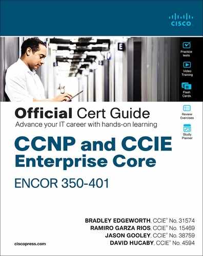
Operating a network requires a specific set of skills. Those skills may include routing knowledge, troubleshooting techniques, and design experience. However, depth of skillsets can vary widely, based on years of experience and size and complexity of the networks that network operators are responsible for. For example, many small networks are very complex, and many very large networks are simple in design and complexity. Having a foundational skillset in key areas can help with the burden of operating and troubleshooting a network. Simply put, a network engineer who has experience with a technology will be more familiar with the technology in the event that the issue or challenge comes up again. This chapter covers some of the most common tools and techniques used to operate and troubleshoot a network. This chapter also covers some of the new software-defined methods of managing, maintaining, and troubleshooting networks. Figure 24-1 shows the basic topology that is used to illustrate these technologies.

Figure 24-1 Basic Topology
Network Diagnostic Tools
Many network diagnostic tools are readily available. This section covers some of the most common tools available and provides use cases and examples of when to use them.
ping
ping is one of the most useful and underrated troubleshooting tools in any network. When following a troubleshooting flow or logic, it is critical to cover the basics first. For example, if a BGP peering adjacency is not coming up, it would make sense to check basic reachability between the two peers prior to doing any deep-dive BGP troubleshooting or debugging. Issues often lie in a lower level of the OSI model; physical layer issues, such as a cable being unplugged, can be found with a quick ping.
The following troubleshooting flow is a quick and basic way to check reachability and try to determine what the issue may be:
Step 1. Gather the facts. If you receive a trouble ticket saying that a remote location is down and cannot access the headquarters, it is important to know what the IP address information for the remote site router or device is. For example, using Figure 24-1, say that R2 is unable to reach the Loopback0 interface on R1. R2’s IP address of its Ethernet0/0 is 10.1.12.2/24.
Step 2. Test reachability by using the ping command. Check to see whether the other end of the link is reachable by issuing the ping 10.1.12.2 command at the command-line interface (CLI).
Step 3. Record the outcome of the ping command and move to the next troubleshooting step. If ping is successful, then the issue isn’t likely related to basic reachability. If ping is unsuccessful, the next step could be checking something more advanced, such as interface issues, routing issues, access lists, or intermediate firewalls.
Example 24-1 illustrates a successful ping between R1 and R2. This example shows five 100-byte ICMP echo request packets sent to 10.1.12.2 with a 2-second timeout. The result is five exclamation points (!!!!!). This means that all five pings were successful within the default parameters, and ICMP echo reply packets were received from the destination. Each ping sent is represented by a single exclamation point (!) or period (.). This means that basic reachability has been verified. The success rate is the percentage of pings that were successful out of the total pings sent. The route trip time is measured in a minimum/average/maximum manner. For example, if five ping packets were sent, and all five were successful, the success rate was 100%; in this case, the minimum/average/maximum were all 1 ms.
Example 24-1 Successful ping Between R1 and R2
R1# ping 10.1.12.2
Type escape sequence to abort.
Sending 5, 100-byte ICMP Echos to 10.1.12.2, timeout is 2 seconds:
!!!!!
Success rate is 100 percent (5/5), round-trip min/avg/max = 1/1/1 ms
It is important to illustrate what an unsuccessful ping looks like as well. Example 24-2 shows an unsuccessful ping to R2’s Ethernet0/0 interface with an IP address of 10.1.12.2.
Example 24-2 Unsuccessful ping Between R1 and R2
R1# ping 10.1.12.2
Type escape sequence to abort.
Sending 5, 100-byte ICMP Echos to 10.1.12.2, timeout is 2 seconds:
.....
Success rate is 0 percent (0/5)
It is easy to count the number of pings when a low number of them are sent. The default is five. However, the parameters mentioned earlier for the ping command can be changed and manipulated to aid in troubleshooting. Example 24-3 shows some of the available options for the ping command on a Cisco device. These options can be seen by using the context sensitive help (?) after the IP address that follows the ping command. This section specifically focuses on the repeat, size, and source options.
Example 24-3 ping 10.1.12.2 Options
R1# ping 10.1.12.2 ?
  data      specify data pattern
  df-bit    enable do not fragment bit in IP header
  repeat    specify repeat count
  size      specify datagram size
  source    specify source address or name
  timeout   specify timeout interval
  tos       specify type of service value
  validate  validate reply data
  <cr>
Suppose that while troubleshooting, a network operator wants to make a change to the network and validate that it resolved the issue at hand. A common way of doing this is to use the repeat option for the ping command. Many times, network operators want to run a continuous or a long ping to see when the destination is reachable. Example 24-4 shows a long ping set with a repeat of 100. In this case, the ping was not working, and then the destination became available—as shown by the 21 periods and the 79 exclamation points.
Example 24-4 ping 10.1.12.2 repeat 100 Command
R1# ping 10.1.12.2 repeat 100
Type escape sequence to abort.
Sending 100, 100-byte ICMP Echos to 10.1.12.2, timeout is 2 seconds:
.....................!!!!!!!!!!!!!!!!!!!!!!!!!!!!!!!!!!!!!!!!!!!!!!!!!
!!!!!!!!!!!!!!!!!!!!!!!!!!!!!!
Success rate is 79 percent (79/100), round-trip min/avg/max = 1/1/1 ms
Another very common use case for the ping command is to send different sizes of packets to a destination. An example might be to send 1500-byte packets with the DF bit set to make sure there are no MTU issues on the interfaces or to test different quality of service policies that restrict certain packet sizes. Example 24-5 shows a ping destined to R2’s Ethernet0/0 interface with an IP address 10.1.12.2 and a packet size of 1500 bytes. The output shows that it was successful.
Example 24-5 ping 10.1.12.2 size 1500 Command
R1# ping 10.1.12.2 size 1500
Type escape sequence to abort.
Sending 5, 1500-byte ICMP Echos to 10.1.12.2, timeout is 2 seconds:
!!!!!
Success rate is 100 percent (5/5), round-trip min/avg/max = 1/1/1 ms
It is sometimes important to source pings from the appropriate interface when sending the pings to the destination. Otherwise, the source IP address used is the outgoing interface. In this topology, there is only one outgoing interface. However, if there were multiple outgoing interfaces, the router would check the routing table to determine the best interface to use for the source of the ping. If a network operator wanted to check a specific path—such as between the Loopback101 interface of R1 and the destination being R2’s Loopback102 interface that has IP address 22.22.22.22—the source-interface option of the ping command could be used. Example 24-6 shows all the options covered thus far (repeat, size, and source-interface) in a single ping command. Multiple options can be used at the same time, as shown here, to simplify troubleshooting. Never underestimated the power of ping!
Example 24-6 ping with Multiple Options
R1# ping 22.22.22.22 source loopback 101 size 1500 repeat 10
Type escape sequence to abort.
Sending 10, 1500-byte ICMP Echos to 22.22.22.22, timeout is 2 seconds:
Packet sent with a source address of 11.11.11.11
!!!!!!!!!!
Success rate is 100 percent (10/10), round-trip min/avg/max = 1/1/1 ms
R1#
An extended ping can take advantage of the same options already discussed as well as some more detailed options for troubleshooting. These options are listed in Table 24-2.
Table 24-2 Extended ping Command Options
Option |
Description |
Protocol |
IP, Novell, AppleTalk, CLNS, and so on; the default is IP |
Target IP address |
Destination IP address of ping packets |
Repeat Count |
Number of ping packets sent; the default is 5 packets |
Datagram Size |
Size of the ping packet; the default is 100 bytes |
Timeout in seconds |
How long a echo reply response is waited for |
Extended Commands |
Yes or No to use extended commands; the default is No, but if Yes is used, more options become available |
Source Address or Interface |
IP address of the source interface or the interface name |
Type of Service (ToS) |
The Type of Service to be used for each probe; 0 is the default |
Set DF bit in IP header |
Sets the Do Not Fragment bit in the IP header; the default is No |
Data Pattern |
The data pattern used in the ping packets; the default is 0xABCD |
Loose, Strict, Record, Timestamp, Verbose |
The options set for the ping packets:
|
Using the same topology shown in Figure 24-1, let’s now look at an extended ping sent from R1’s Loopback101 interface, destined to R2’s Loopback123 interface. The following list provides the extended options that will be used:
IP
Repeat count of 1
Datagram size of 1500 bytes
Timeout of 1 second
Source Interface of Loopback101
Type of Service of 184
Setting the DF bit in the IP Header
Data pattern 0xABBA
Timestamp and default of Verbose
Example 24-7 shows an extended ping using all these options and the output received from the tool at the command line. A repeat count of 1 is used in this example just to make the output more legible. Usually, this is 5 at the minimum or a higher number, depending on what is being diagnosed. Most common interface MTU settings are set at 1500 bytes. Setting the MTU in an extended ping and setting the DF bit in the IP header can help determine whether there are MTU settings in the path that are not set appropriately. A good example of when to use this is with tunneling. It is important to account for the overhead of the tunnel technology, which can vary based on the tunnel technology being used. Specifying a Type of Service of 184 in decimal translates to Expedited Forwarding or (EF) per-hop behavior (PHB). This can be useful when testing real-time quality of service (QoS) policies in a network environment. However, some service providers do not honor pings or ICMP traffic marked with different PHB markings. Setting Data Patterns can help when troubleshooting framing errors, line coding, or clock signaling issues on serial interfaces. Service providers often ask network operators to send all 0s (0x0000) or all 1s (0xffff) during testing, depending on the issues they suspect. Finally, a timestamp is set in this example, in addition to the default Verbose output. This gives a clock timestamp of when the destination sent an echo reply message back to the source.
Example 24-7 Extended ping with Multiple Options
R1# ping
Protocol [ip]:
Target IP address: 22.22.22.23
Repeat count [5]: 1
Datagram size [100]: 1500
Timeout in seconds [2]: 1
Extended commands [n]: yes
Source address or interface: Loopback101
Type of service [0]: 184
Set DF bit in IP header? [no]: yes
Validate reply data? [no]:
Data pattern [0xABCD]: 0xABBA
Loose, Strict, Record, Timestamp, Verbose[none]: Timestamp
Number of timestamps [ 9 ]: 3
Loose, Strict, Record, Timestamp, Verbose[TV]:
Sweep range of sizes [n]:
Type escape sequence to abort.
Sending 1, 1500-byte ICMP Echos to 22.22.22.23, timeout is 1 seconds:
Packet sent with a source address of 11.11.11.11
Packet sent with the DF bit set
Packet has data pattern 0xABBA
Packet has IP options:  Total option bytes= 16, padded length=16
 Timestamp: Type 0.  Overflows: 0 length 16, ptr 5
  >>Current pointer<<
  Time= 16:00:00.000 PST (00000000)
  Time= 16:00:00.000 PST (00000000)
  Time= 16:00:00.000 PST (00000000)

Reply to request 0 (1 ms).  Received packet has options
 Total option bytes= 16, padded length=16
 Timestamp: Type 0.  Overflows: 1 length 16, ptr 17
  Time=*08:18:41.697 PST (838005A1)
  Time=*08:18:41.698 PST (838005A2)
  Time=*08:18:41.698 PST (838005A2)
  >>Current pointer<<

Success rate is 100 percent (1/1), round-trip min/avg/max = 1/1/1 ms
ping and extended ping are very useful and powerful troubleshooting tools that you are likely to use daily. The information gained from using the ping command can help lead network operations staff to understand where an issue may exist within the network environment. More often than not, ping is used as a quick verification tool to confirm or narrow down the root cause of a network issue that is causing reachability problems.
traceroute
traceroute is another common troubleshooting tool. traceroute is often used to troubleshoot when trying to determine where traffic is failing as well as what path traffic takes throughout the network. traceroute shows the IP addresses or DNS names of the hops between the source and destination. It also shows how long it takes to reach the destination at each hop, measured in milliseconds. This tool is frequently used when more than one path is available to the destination or when there is more than one hop to the destination. Using the same topology shown in Figure 24-1, Example 24-8 shows a traceroute from R1 to R2’s Loopback102 address of 22.22.22.22. Example 24-8 shows a successful traceroute from R1 to R2’s Loopback102 interface. The output shows that the traceroute to 22.22.22.22 was sent to the next hop of 10.1.12.2 and was successful. Three probes were sent, and the second one timed out.
Example 24-8 Basic traceroute to R2 Loopback102
R1# traceroute 22.22.22.22
Type escape sequence to abort.
Tracing the route to 22.22.22.22
VRF info: (vrf in name/id, vrf out name/id)
  1 10.1.12.2 0 msec *  1 msec
Example 24-9 shows an unsuccessful traceroute. There are many reasons for unsuccessful traceroutes; however, one of the most common is a missing route or down interface. Example 24-9 illustrates a failed traceroute due to a missing route or mistyped destination. Notice that when a timeout has occurred, traceroute displays an asterisk. By default, traceroute tries up to 30 times/hops before completing.
Example 24-9 Basic traceroute to a Nonexistent Route
R1# traceroute 22.22.22.23
Type escape sequence to abort.
Tracing the route to 22.22.22.23
VRF info: (vrf in name/id, vrf out name/id)
  1  *  *  *
  2  *  *  *
  3  *  *  *
  4  *  *  *
  5  *  *  *
  6  *  *  *
  7  *  *  *
  8  *  *  *
  9  *  *  *
 10  *  *  *
 11  *  *  *
 12  *  *  *
 13  *  *  *
 14  *  *  *
 15  *  *  *
 16  *  *  *
 17  *  *  *
 18  *  *  *
 19  *  *  *
 20  *  *  *
 21  *  *  *
 22  *  *  *
 23  *  *  *
 24  *  *  *
 25  *  *  *
 26  *  *  *
 27  *  *  *
 28  *  *  *
 29  *  *  *
 30  *  *  *
Example 24-10 shows the R1 routing table. This output shows that R1 has a /32 host route to 22.22.22.22 using OSPF. However, there is no route for 22.22.22.23/32, which is why the traceroute is failing.
Example 24-10 R1 Routing Table
R1# show ip route
Codes: L - local, C - connected, S - static, R - RIP, M - mobile, B - BGP
       D - EIGRP, EX - EIGRP external, O - OSPF, IA - OSPF inter area
       N1 - OSPF NSSA external type 1, N2 - OSPF NSSA external type 2
       E1 - OSPF external type 1, E2 - OSPF external type 2
       i - IS-IS, su - IS-IS summary, L1 - IS-IS level-1, L2 - IS-IS level-2
       ia - IS-IS inter area, * - candidate default, U - per-user static route
       o - ODR, P - periodic downloaded static route, H - NHRP, l - LISP
       a - application route
       + - replicated route, % - next hop override

Gateway of last resort is not set

      10.0.0.0/8 is variably subnetted, 2 subnets, 2 masks
C        10.1.12.0/24 is directly connected, Ethernet0/0
L        10.1.12.1/32 is directly connected, Ethernet0/0
      11.0.0.0/32 is subnetted, 1 subnets
C        11.11.11.11 is directly connected, Loopback101
      22.0.0.0/32 is subnetted, 1 subnets
O IA     22.22.22.22 [110/11] via 10.1.12.2, 01:58:55, Ethernet0/0
Furthermore, if a less specific route is added to R1 that points to 22.0.0.0/8 or 22.0.0.0 255.0.0.0, the traceroute returns a “host unreachable” message. This is because there is a route to the next hop, R2 (10.1.12.2), but once the traceroute gets to R2, there is no interface or route to 22.22.22.23/32, and the traceroute fails. Example 24-11 shows this scenario.
Example 24-11 Adding a Less Specific Route on R1
R1# configure terminal
Enter configuration commands, one per line.  End with CNTL/Z.
R1(config)# ip route 22.0.0.0 255.0.0.0 10.1.12.2
R1(config)# end
R1# traceroute 22.22.22.23
Type escape sequence to abort.
Tracing the route to 22.22.22.23
VRF info: (vrf in name/id, vrf out name/id)
  1 10.1.12.2 0 msec 0 msec 0 msec
  2 10.1.12.2 !H  *  !H
If a new loopback interface were added to R2 with the IP address 22.22.22.23 255.255.255.0, the traceroute would be successful. Example 24-12 shows the new Loopback123 interface configured on R2. Note that the response in Example 24-11 includes !H, which means R1 received an ICMP “destination host unreachable” message from R2. This is what happens when there is not a route present to the IP address.
Example 24-12 Adding a Loopback123 Interface on R2
R2# configure terminal
Enter configuration commands, one per line.  End with CNTL/Z.
R2(config)# int loopback 123
R2(config-if)# ip add 22.22.22.23 255.255.255.255
R2(config-if)# end
Now that the new Loopback123 interface is configured on R2, it is important to circle back and rerun the traceroute from R1 to the 22.22.22.23 address to see if it is successful. Example 24-13 shows a successful traceroute from R1 to Loopback123 on R2.
Example 24-13 Adding a Loopback123 Interface on R2
R1# traceroute 22.22.22.23
Type escape sequence to abort.
Tracing the route to 22.22.22.23
VRF info: (vrf in name/id, vrf out name/id)
  1 10.1.12.2 0 msec *  0 msec
Another great benefit of traceroute is that it has options available, much like the ping command. These options can also be discovered by leveraging the context-sensitive help (?) from the command-line interface. Example 24-14 shows the list of available options to the traceroute command. This section focuses on the port, source, timeout, and probe options.
Example 24-14 Available traceroute Options
R1# traceroute 22.22.22.23 ?
  numeric  display numeric address
  port     specify port number
  probe    specify number of probes per hop
  source   specify source address or name
  timeout  specify time out
  ttl      specify minimum and maximum ttl
  <cr>
There are times when using some of the options available with traceroute may be useful (for example, if a network operator wants to change the port that the first probe is sent out on or source the traceroute from a different interface, such as a loopback interface). There are also times when there might be a reason to send a different number of probes per hop with different timeout timers rather than the default of three probes. As with the ping command, multiple traceroute options can be used at the same time. Example 24-15 shows the traceroute command being used on R1 to R2’s Loopback123 interface with the port, probe, source, and timeout options all set.
Example 24-15 traceroute to R2 Loopback123 with Options
R1# traceroute 22.22.22.23 port 500 source loopback101 probe 5 timeout 10
Type escape sequence to abort.
Tracing the route to 22.22.22.23
VRF info: (vrf in name/id, vrf out name/id)
  1 10.1.12.2 1 msec *  0 msec *  0 msec
Much like the extended ping command covered earlier in this chapter, there is an extended traceroute command, and it has a number of detailed options available. Those options are listed in Table 24-3.
Table 24-3 Extended traceroute Command Options
Option |
Description |
Protocol |
IP, Novell, AppleTalk, CLNS, and so on; the default is IP |
Target IP address |
Destination IP address of ping packets |
Numeric display |
Shows only the numeric display rather than numeric and symbolic display |
Timeout in Seconds |
Time that is waited for a reply to a probe; the default is 3 seconds |
Probe count |
Number of probes sent at each hop; the default is 3 |
Source Address |
IP address of the source interface |
Minimum Time-to-live |
TTL value of the first set of probes; can be used to hide topology information or known hops |
Maximum Time-to-live |
Maximum number of hops; the default is 30 |
Port number |
Destination port number of probes; the default is 33434 |
Loose, Strict, Record, Timestamp, Verbose |
The options set for the traceroute probes:
|
Using the same topology shown earlier in the chapter, in Figure 24-1, an extended traceroute will be sent from R1’s Loopback101 interface destined to R2’s Loopback123 interface. The following extended options will be used:
IP
Source Interface of Loopback101
Timeout of 2 seconds
Probe count of 1
Port number 12345
Timestamp and default of Verbose
Example 24-16 shows an extended traceroute using all these options and the output received from the tool at the command line. A probe count of 1 is used in this example just to make the output more legible. Usually, this is 3 by default, and it can be increased, depending on what is being diagnosed.
Example 24-16 Extended traceroute to R2 Loopback123 with Options
R1# traceroute
Protocol [ip]:
Target IP address: 22.22.22.23
Source address: 11.11.11.11
Numeric display [n]:
Timeout in seconds [3]: 2
Probe count [3]: 1
Minimum Time to Live [1]:
Maximum Time to Live [30]:
Port Number [33434]: 12345
Loose, Strict, Record, Timestamp, Verbose[none]: Timestamp
Number of timestamps [ 9 ]:
Loose, Strict, Record, Timestamp, Verbose[TV]:
Type escape sequence to abort.
Tracing the route to 22.22.22.23
VRF info: (vrf in name/id, vrf out name/id)
  1 10.1.12.2 1 msec
Received packet has options
Total option bytes= 40, padded length=40
 Timestamp: Type 0.  Overflows: 0 length 40, ptr 13
  Time=*09:54:37.983 PST (83D7DB1F)
  Time=*09:54:37.983 PST (83D7DB1F)
  >>Current pointer<<
  Time= 16:00:00.000 PST (00000000)
  Time= 16:00:00.000 PST (00000000)
  Time= 16:00:00.000 PST (00000000)
  Time= 16:00:00.000 PST (00000000)
  Time= 16:00:00.000 PST (00000000)
  Time= 16:00:00.000 PST (00000000)
  Time= 16:00:00.000 PST (00000000)
Debugging
Debugging can be a very powerful part of troubleshooting complex issues in a network. Debugging is also informational. This section provides some basic OSPF debugging examples and illustrates how to use debugging when trying to narrow down issues in a network.
One of the most common use cases for debugging is when there is a need to see things at a deeper level (such as when routing protocols are having adjacency issues). There is a normal flow that is taken from a troubleshooting perspective, depending on the routing protocol. However, there are times when these steps have been taken, and the issue is not evident. With OSPF, for example, when troubleshooting adjacency issues, it is very helpful to have debugging experience. Using the simple topology shown in Figure 24-2, in this section, debugging is used to fix a couple issues in the OSPF area 0.
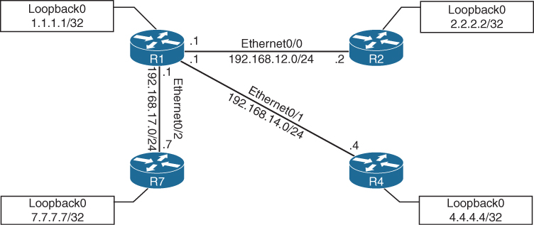
Figure 24-2 Debugging Topology
Some of the common OSPF adjacency issues can be resolved by using debugging. The following issues are covered in this section:
MTU issues
Incorrect interface types
Improperly configured network mask
From the output of the show ip ospf neighbor command on R1 in Example 24-17, it can be seen that the neighbor adjacency to R4 is in the INIT state. If the command is run after a few seconds, the state changes to EXCHANGE but quickly cycles back to the INIT state when the command is run again.
Example 24-17 Output of the show ip ospf neighbor Command
R1# show ip ospf neighbor

Neighbor ID     Pri   State           Dead Time   Address         Interface
7.7.7.7           0   FULL/  -        00:00:31    192.168.17.7    Ethernet0/2
4.4.4.4           0   INIT/  -        00:00:37    192.168.14.4    Ethernet0/1
2.2.2.2           0   FULL/  -        00:00:33    192.168.12.2    Ethernet0/0
R1# show ip ospf neighbor

Neighbor ID     Pri   State           Dead Time   Address         Interface
7.7.7.7           0   FULL/  -        00:00:33    192.168.17.7    Ethernet0/2
4.4.4.4           0   EXCHANGE/  -    00:00:37    192.168.14.4    Ethernet0/1
2.2.2.2           0   FULL/  -        00:00:32    192.168.12.2    Ethernet0/0
R1# show ip ospf neighbor

Neighbor ID     Pri   State           Dead Time   Address         Interface
7.7.7.7           0   FULL/  -        00:00:31    192.168.17.7    Ethernet0/2
4.4.4.4           0   INIT/  -        00:00:38    192.168.14.4    Ethernet0/1
2.2.2.2           0   FULL/  -        00:00:39    192.168.12.2    Ethernet0/0
A typical approach to this line of troubleshooting is to log into both devices and look at the logs or the running configuration. Although this approach may reveal the issue at hand, it may not be the most efficient way to troubleshoot. For example, a considerable amount of time is needed to log into multiple devices and start combing through the configurations to see what may be missing or misconfigured. In the next example, debugging is used on R1 to try to determine what the issue is. Example 24-18 shows the output of the debug ip ospf adj command. This command is used to reveal messages that are exchanged during the OSPF adjacency process.
Example 24-18 Output of the debug ip ospf adj Command on R1
R1# debug ip ospf adj
OSPF adjacency debugging is on
R1#
19:20:42.559: OSPF-1 ADJ   Et0/1: Rcv DBD from 4.4.4.4 seq 0x247A opt 0x52 flag 0x7
len 32  mtu 1400 state EXCHANGE
19:20:42.559: OSPF-1 ADJ   Et0/1: Nbr 4.4.4.4 has smaller interface MTU
19:20:42.559: OSPF-1 ADJ   Et0/1: Send DBD to 4.4.4.4 seq 0x247A opt 0x52 flag 0x2
len 152
R1#un all
All possible debugging has been turned off
With one debug command, it was easy to determine the root cause of the failed adjacency. The output of the debug ip ospf adj command in Example 24-18 clearly states that it received a Database Descriptor packet from the neighbor 4.4.4.4, and that the neighbor 4.4.4.4 has a smaller interface MTU of 1400. If the same debug command were run on R4, the output would be similar but show the reverse. Example 24-19 shows the output of the debug ip ospf adj command on R4 with the relevant fields highlighted.
Example 24-19 Output of the debug ip ospf adj Command on R4
R4# debug ip ospf adj
OSPF adjacency debugging is on
R4#
19:28:18.102: OSPF-1 ADJ   Et0/1: Send DBD to 1.1.1.1 seq 0x235C opt 0x52 flag 0x7
len 32
19:28:18.102: OSPF-1 ADJ   Et0/1: Retransmitting DBD to 1.1.1.1 [23]
19:28:18.102: OSPF-1 ADJ   Et0/1: Rcv DBD from 1.1.1.1 seq 0x235C opt 0x52 flag 0x2
len 152  mtu 1500 state EXSTART
19:28:18.102: OSPF-1 ADJ   Et0/1: Nbr 1.1.1.1 has larger interface MTU
R4#un all
All possible debugging has been turned off
The output of the debug command in Example 24-19 shows that R1 has an MTU size of 1500, which is larger than the locally configured MTU of 1400 on R4. This is a really quick way of troubleshooting this type of issue with adjacency formation.
The second issue to cover with adjacency formation is OSPF network type mismatch, which is a very common reason for neighbor adjacency issues. Often this is simply a misconfiguration issue when setting up the network. When the debug ip ospf hello command is used on R1, everything appears to be normal: Hellos are sent to the multicast group 224.0.0.5 every 10 seconds. Example 24-20 shows the output of the debug command on R1.
Example 24-20 Output of the debug ip ospf hello Command on R1
R1# debug ip ospf hello
OSPF hello debugging is on
R1#
19:47:46.976: OSPF-1 HELLO Et0/0: Send hello to 224.0.0.5 area 0 from 192.168.12.1
19:47:47.431: OSPF-1 HELLO Et0/1: Send hello to 224.0.0.5 area 0 from 192.168.14.1
19:47:48.363: OSPF-1 HELLO Et0/2: Send hello to 224.0.0.5 area 0 from 192.168.17.1
R1#
19:47:50.582: OSPF-1 HELLO Et0/0: Rcv hello from 2.2.2.2 area 0 192.168.12.2
19:47:51.759: OSPF-1 HELLO Et0/2: Rcv hello from 7.7.7.7 area 0 192.168.17.7
R1#
19:47:56.923: OSPF-1 HELLO Et0/0: Send hello to 224.0.0.5 area 0 from 192.168.12.1
19:47:57.235: OSPF-1 HELLO Et0/1: Send hello to 224.0.0.5 area 0 from 192.168.14.1
19:47:58.159: OSPF-1 HELLO Et0/2: Send hello to 224.0.0.5 area 0 from 192.168.17.1
R1#
19:47:59.776: OSPF-1 HELLO Et0/0: Rcv hello from 2.2.2.2 area 0 192.168.12.2
19:48:01.622: OSPF-1 HELLO Et0/2: Rcv hello from 7.7.7.7 area 0 192.168.17.7
R1#un all
All possible debugging has been turned off
However, the situation is different if we issue the same debug command on R4. Example 24-21 shows the issue called out right in the debug output on R4. Based on the output, we can see that the hello parameters are mismatched. The output shows that R4 is receiving a dead interval of 40, while it has a configured dead interval of 120. We can also see that the hello interval R4 is receiving is 10, and the configured hello interval is 30. By default, the dead interval is 4 times the hello interval.
Example 24-21 Output of the debug ip ospf hello Command on R4
R4# debug ip ospf hello
OSPF hello debugging is on
R4#
19:45:45.127: OSPF-1 HELLO Et0/1: Rcv hello from 1.1.1.1 area 0 192.168.14.1
19:45:45.127: OSPF-1 HELLO Et0/1: Mismatched hello parameters from 192.168.14.1
19:45:45.127: OSPF-1 HELLO Et0/1: Dead R 40 C 120, Hello R 10 C 30
19:45:45.259: OSPF-1 HELLO Et0/3: Rcv hello from 7.7.7.7 area 0 192.168.47.7
R4#
19:45:48.298: OSPF-1 HELLO Et0/0: Send hello to 224.0.0.5 area 0 from 192.168.34.4
19:45:48.602: OSPF-1 HELLO Et0/0: Rcv hello from 3.3.3.3 area 0 192.168.34.3
R4#un all
All possible debugging has been turned off
Different network types have different hello intervals and dead intervals. Table 24-4 highlights the different hello and dead interval times based on the different OSPF network types.
Table 24-4 OSPF Network Types and Hello/Dead Intervals
Network Type |
Hello Interval (in seconds) |
Dead Interval (in seconds) |
Broadcast |
10 |
40 |
Non-broadcast |
30 |
120 |
Point-to-point |
10 |
40 |
Point-to-Multipoint |
30 |
120 |
The issue could be simply mismatched network types or mismatched hello or dead intervals. The show ip ospf interface command shows what the configured network types and hello and dead intervals are. Example 24-22 shows the output of this command on R4.
Example 24-22 Output of the show ip ospf interface Command on R4
R4# show ip ospf interface ethernet0/1
Ethernet0/1 is up, line protocol is up
  Internet Address 192.168.14.4/24, Area 0, Attached via Network Statement
  Process ID 1, Router ID 4.4.4.4, Network Type POINT_TO_MULTIPOINT, Cost: 10
  Topology-MTID    Cost    Disabled    Shutdown      Topology Name
        0           10        no          no            Base
  Transmit Delay is 1 sec, State POINT_TO_MULTIPOINT
  Timer intervals configured, Hello 30, Dead 120, Wait 120, Retransmit 5
    oob-resync timeout 120
    Hello due in 00:00:05
  Supports Link-local Signaling (LLS)
  Cisco NSF helper support enabled
  IETF NSF helper support enabled
  Index 2/2, flood queue length 0
  Next 0x0(0)/0x0(0)
  Last flood scan length is 1, maximum is 2
  Last flood scan time is 0 msec, maximum is 1 msec
  Neighbor Count is 0, Adjacent neighbor count is 0
  Suppress hello for 0 neighbor(s)
Simply changing the network type on R4 interface Ethernet0/1 back to the default of Broadcast fixes the adjacency issue in this case. This is because R1 is configured as Broadcast, and now the hello and dead intervals will match. Example 24-23 shows the ip ospf network-type broadcast command issued to change the network type to Broadcast on the Ethernet0/1 interface and the neighbor adjacency coming up. It is also verified with the do show ip ospf neighbor command.
Example 24-23 Changing the Network Type on R4
R4# configure terminal
Enter configuration commands, one per line.  End with CNTL/Z.
R4(config)# interface ethernet0/1
R4(config-if)# ip ospf network broadcast
R4(config-if)#
20:28:51.904: %OSPF-5-ADJCHG: Process 1, Nbr 1.1.1.1 on Ethernet0/1 from LOADING to
FULL, Loading Done
R4(config-if)# do show ip ospf neighbor

Neighbor ID     Pri   State           Dead Time   Address         Interface
7.7.7.7           0   FULL/  -        00:00:32    192.168.47.7    Ethernet0/3
1.1.1.1           1   FULL/BDR        00:00:39    192.168.14.1    Ethernet0/1
3.3.3.3           0   FULL/  -        00:00:33    192.168.34.3    Ethernet0/0
The final use case for using debugging to solve OSPF adjacency issues involves improper configuration of IP addresses and subnet masks on an OSPF interface. To troubleshoot this without having to look through running configurations or at a specific interface, you can use the same debug ip ospf hello command covered earlier in this section. Example 24-24 shows the output of running the show ip ospf neighbor command on R1. It indicates that there is no OSPF adjacency to R4 when there certainly should be one. The adjacency is stuck in INIT mode. In Example 24-24, the debug ip ospf hello command and the debug ip ospf adj command are enabled on R1 to see what is going on. The output shows a message that states, “No more immediate hello for nbr 4.4.4.4, which has been sent on this intf 2 times.” This indicates that something is wrong between R1 and R4.
Example 24-24 show ip ospf neighbor, debug ip ospf hello, and debug ip ospf adj Commands on R1
R1# show ip ospf neighbor

Neighbor ID     Pri   State           Dead Time   Address         Interface
7.7.7.7           0   FULL/  -        00:00:34    192.168.17.7    Ethernet0/2
4.4.4.4           0   INIT/  -        00:00:30    192.168.14.4    Ethernet0/1
2.2.2.2           0   FULL/  -        00:00:37    192.168.12.2    Ethernet0/0
R1#
R1# deb ip os hello
OSPF hello debugging is on
R1# deb ip ospf adj
OSPF adjacency debugging is on
R1#
20:55:02.465: OSPF-1 HELLO Et0/0: Send hello to 224.0.0.5 area 0 from 192.168.12.1
20:55:03.660: OSPF-1 HELLO Et0/0: Rcv hello from 2.2.2.2 area 0 192.168.12.2
20:55:04.867: OSPF-1 HELLO Et0/1: Send hello to 224.0.0.5 area 0 from 192.168.14.1
20:55:05.468: OSPF-1 HELLO Et0/1: Rcv hello from 4.4.4.4 area 0 192.168.14.4
20:55:05.468: OSPF-1 HELLO Et0/1: No more immediate hello for nbr 4.4.4.4, which has
been sent on this intf 2 times
R1#
20:55:06.051: OSPF-1 HELLO Et0/2: Send hello to 224.0.0.5 area 0 from 192.168.17.1
R1#
20:55:08.006: OSPF-1 HELLO Et0/2: Rcv hello from 7.7.7.7 area 0 192.168.17.7

R1#
R1# undebug all
All possible debugging has been turned off
Issuing the same debug commands on R4 provides the output shown in Example 24-25; the issue is mismatched hello parameters. R4 is receiving a network of 255.255.255.0, but it has a network mask of 255.255.255.248 locally configured. This causes an adjacency issue even though the hello and dead intervals are configured to match.
Example 24-25 debug ip ospf hello and debug ip ospf adj Commands on R4
R4# deb ip ospf hello
OSPF hello debugging is on
R4# deb ip os ad
OSPF adjacency debugging is on
R4#
21:05:50.863: OSPF-1 HELLO Et0/0: Rcv hello from 3.3.3.3 area 0 192.168.34.3
21:05:51.318: OSPF-1 HELLO Et0/1: Send hello to 224.0.0.5 area 0 from 192.168.14.4
21:05:51.859: OSPF-1 HELLO Et0/3: Send hello to 224.0.0.5 area 0 from 192.168.47.4
R4#
21:05:53.376: OSPF-1 HELLO Et0/0: Send hello to 224.0.0.5 area 0 from 192.168.34.4
R4#
21:05:56.906: OSPF-1 HELLO Et0/3: Rcv hello from 7.7.7.7 area 0 192.168.47.7
R4#
21:05:57.927: OSPF-1 HELLO Et0/1: Rcv hello from 1.1.1.1 area 0 192.168.14.1
21:05:57.927: OSPF-1 HELLO Et0/1: Mismatched hello parameters from 192.168.14.1
21:05:57.927: OSPF-1 HELLO Et0/1: Dead R 40 C 40, Hello R 10 C 10 Mask R
255.255.255.0 C 255.255.255.248
R4#
21:06:00.255: OSPF-1 HELLO Et0/0: Rcv hello from 3.3.3.3 area 0 192.168.34.3
21:06:00.814: OSPF-1 HELLO Et0/1: Send hello to 224.0.0.5 area 0 from 192.168.14.4
21:06:01.047: OSPF-1 HELLO Et0/3: Send hello to 224.0.0.5 area 0 from 192.168.47.4
R4# undebug all
All possible debugging has been turned off
R4#
To resolve this issue, the network mask on the Ethernet0/1 interface of R4 needs to be changed to match the one that R1 has configured and is sending to R4 through OSPF hellos. Example 24-26 shows the network mask being changed on the R4 Ethernet0/1 interface and the OSPF adjacency coming up. This is then verified with the do show ip ospf neighbor command.
Example 24-26 Network Mask Change and show ip ospf neighbor on R4
R4# configure terminal
Enter configuration commands, one per line.  End with CNTL/Z.
R4(config)# interface ethernet0/1
R4(config-if)# ip address 192.168.14.4 255.255.255.0
R4(config-if)#
21:14:15.598: %OSPF-5-ADJCHG: Process 1, Nbr 1.1.1.1 on Ethernet0/1 from LOADING to
FULL, Loading Done
R4(config-if)# do show ip ospf neighbor
Neighbor ID     Pri   State           Dead Time   Address         Interface
1.1.1.1           1   FULL/BDR        00:00:38    192.168.14.1    Ethernet0/1
7.7.7.7           0   FULL/  -        00:00:37    192.168.47.7    Ethernet0/3
3.3.3.3           0   FULL/  -        00:00:30    192.168.34.3    Ethernet0/0
R4(config-if)#
Conditional Debugging
As mentioned earlier in this chapter, debugging can be very informational. Sometimes, there is too much information, and it is important to know how to restrict the debug commands and limit the messages to what is appropriate for troubleshooting the issue at hand. Often, networking engineers or operators are intimidated by the sheer number of messages that can be seen while debugging. In the past, routers and switches didn’t have as much memory and CPU as they do today, and running debug (especially running multiple debug commands simultaneously) could cause a network device to become unresponsive or crash, and it could even cause an outage.
Conditional debugging can be used to limit the scope of the messages that are being returned to the console or syslog server. A great example of this is the debug ip packet command. Issuing this command on a router that is in production could send back a tremendous number of messages. One way to alleviate this issue is to attach an access list to the debug command to limit the scope of messages to the source or destination specified within the access list. For example, say that you configure an access list that focuses on any traffic to or from the 192.168.14.0/24 network. This can be done using standard or extended access lists. The options for the debug ip packet command are as follows:
<1-199>: Standard access list
<1300-2699>: Access list with expanded range
detail: More debugging detail
To showcase the power of conditional debugging, Example 24-27 uses a standard access list to limit the messages to the console and filter solely on traffic to and from the 192.168.14.0/24 subnet.
Example 24-27 Conditional Debugging IP Packet for 192.168.14.0/24 on R4
R4(config)# access-list 100 permit ip any 192.168.14.0 0.0.0.255
R4(config)# access-list 100 permit ip 192.168.14.0 0.0.0.255 any
R4# debug ip packet 100
IP packet debugging is on for access list 100
R4#
21:29:58.118: IP: s=192.168.14.1 (Ethernet0/1), d=224.0.0.2, len 62, rcvd 0
21:29:58.118: IP: s=192.168.14.1 (Ethernet0/1), d=224.0.0.2, len 62, input feature,
packet consumed, MCI Check(104), rtype 0, forus FALSE, sendself FALSE, mtu 0, fwdchk
  FALSE
R4#
21:30:00.418: IP: s=192.168.14.4 (local), d=224.0.0.2 (Ethernet0/1), len 62, sending
  broad/multicast
21:30:00.418: IP: s=192.168.14.4 (local), d=224.0.0.2 (Ethernet0/1), len 62, sending
  full packet
R4#
21:30:01.964: IP: s=192.168.14.1 (Ethernet0/1), d=224.0.0.2, len 62, rcvd 0
21:30:01.964: IP: s=192.168.14.1 (Ethernet0/1), d=224.0.0.2, len 62, input feature,
   packet consumed, MCI Check(104), rtype 0, forus FALSE, sendself FALSE, mtu 0,
   fwdchk FALSE
21:30:02.327: IP: s=192.168.14.1 (Ethernet0/1), d=224.0.0.5, len 80, rcvd 0
21:30:02.327: IP: s=192.168.14.1 (Ethernet0/1), d=224.0.0.5, len 80, input feature,
   packet consumed, MCI Check(104), rtype 0, forus FALSE, sendself FALSE, mtu 0,
   fwdchk FALSE
R4#
21:30:03.263: IP: s=192.168.14.4 (local), d=224.0.0.5 (Ethernet0/1), len 80, sending
  broad/multicast
21:30:03.263: IP: s=192.168.14.4 (local), d=224.0.0.5 (Ethernet0/1), len 80, sending
  full packet
R4# un
21:30:04.506: IP: s=192.168.14.4 (local), d=224.0.0.2 (Ethernet0/1), len 62, sending
  broad/multicast
21:30:04.506: IP: s=192.168.14.4 (local), d=224.0.0.2 (Ethernet0/1), len 62, sending
  full packet
R4# undebug all
All possible debugging has been turned off
R4#
Another common method of conditional debugging is to debug on a specific interface. This is extremely useful when trying to narrow down a packet flow between two hosts. Imagine that a network engineer is trying to debug a traffic flow between R1’s Ethernet0/1 interface with source IP address 192.168.14.1/24 that is destined to R4’s Loopback0 interface with IP address 4.4.4.4/32. One way to do this would certainly be to change the access list 100 to reflect these source and destination IP addresses. However, because the access list is looking for any traffic sourced or destined to the 192.168.14.0/24 network, this traffic flow would fall into matching that access list. Using conditional debugging on the Loopback0 interface of R4 would be a simple way of meeting these requirements. Example 24-28 shows the conditional debugging on R4. When that is in place, a ping on R1 sourced from the Ethernet0/1 interface matches the conditions set on R4.
Example 24-28 Conditional Loopback0 Interface Debugging IP Packet for 192.168.14.0/24 on R4
R4# debug interface Loopback0
Condition 1 set
R4#
R4#
R4# debug ip packet 100
IP packet debugging is on for access list 100
R4#
R4#
R4# show debug
Generic IP:
  IP packet debugging is on for access list 100
Condition 1: interface Lo0 (1 flags triggered)
        Flags: Lo0

R4#
21:39:59.033: IP: tableid=0, s=192.168.14.1 (Ethernet0/3), d=4.4.4.4 (Loopback0),
routed via RIB
21:39:59.033: IP: s=192.168.14.1 (Ethernet0/3), d=4.4.4.4, len 100, stop process pak
  for forus packet
21:39:59.033: IP: tableid=0, s=192.168.14.1 (Ethernet0/3), d=4.4.4.4 (Loopback0),
  routed via RIB
21:39:59.033: IP: s=192.168.14.1 (Ethernet0/3), d=4.4.4.4, len 100, stop process pak
  for forus packet
21:39:59.033: IP: tableid=0, s=192.168.14.1 (Ethernet0/3), d=4.4.4.4 (Loopback0),
  routed via RIB
21:39:59.033: IP: s=192.168.14.1 (Ethernet0/3), d=4.4.4.4, len 100, stop process pak
  for forus packet
R4#
21:39:59.034: IP: tableid=0, s=192.168.14.1 (Ethernet0/3), d=4.4.4.4 (Loopback0),
  routed via RIB
21:39:59.034: IP: s=192.168.14.1 (Ethernet0/3), d=4.4.4.4, len 100, stop process pak
  for forus packet
21:39:59.034: IP: tableid=0, s=192.168.14.1 (Ethernet0/3), d=4.4.4.4 (Loopback0),
  routed via RIB
21:39:59.034: IP: s=192.168.14.1 (Ethernet0/3), d=4.4.4.4, len 100, stop process pak
  for forus packet
R4# undebug all
All possible debugging has been turned off
R4# undebug interface loopback0
This condition is the last interface condition set.
Removing all conditions may cause a flood of debugging
messages to result, unless specific debugging flags
are first removed.

Proceed with removal? [yes/no]: yes
Condition 1 has been removed
It is important to note that even if all debugging has been turned off using the undebug all command, the interface conditions set for Loopback0 on R4 remain. The way to remove this condition is to use the undebug interface loopback0 command on R4. Once this is executed, the user is asked to confirm whether to proceed with removing the condition. The conditions can be removed while live debug commands are still running, and the operating system wants to indicate that the user might receive a flood of debug messages when the condition is removed. Although there are many more debug operations available, understanding the fundamental steps outlined here helps take the fear out of using this powerful diagnostic tool when troubleshooting issues that arise in the network environment.
Simple Network Management Protocol (SNMP)
Network operations teams often have to rely on reactive alerting from network devices to be notified when something is happening—such as something failing or certain events happening on a device. The typical tool for this is Simple Network Management Protocol (SNMP). SNMP can also be used to configure devices, although this use is less common. More often when network engineering teams need to configure devices, configuration management tools such as Cisco Prime Infrastructure are used.
This section focuses on SNMP from an alerting perspective and provides some configuration examples for enabling SNMP and some basic functionality of the protocol. SNMP sends unsolicited traps to an SNMP collector or network management system (NMS). These traps are in response to something that happened in the network. For example, traps may be generated for link status events, improper user authentication, and power supply failures. These events are defined in the SNMP Management Information Base (MIB). The MIB can be thought of as a repository of device parameters that can be used to trigger alerts. There are currently three versions of SNMP. Table 24-5 lists the versions and their differences.
Table 24-5 SNMP Version Comparison
Version |
Level |
Authentication |
Encryption |
Result |
SNMPv1 |
noAuthNoPriv |
Community string |
No |
Uses a community string match for authentication. |
SNMPv2c |
noAuthNoPriv |
Community string |
No |
Uses a community string match for authentication. |
SNMPv3 |
noAuthNoPriv |
Username |
No |
Uses a username match for authentication. |
SNMPv3 |
authNoPriv |
Message Digest 5 (MD5) or Secure Hash Algorithm (SHA) |
No |
Provides authentication based on the HMAC-MD5 or HMAC-SHA algorithms. |
SNMPv3 |
authPriv (requires the cryptographic software image) |
MD5 or SHA |
Data Encryption Standard (DES) or Advanced Encryption Standard (AES) |
Provides authentication based on the HMAC-MD5 or HMAC-SHA algorithms. Allows specifying the User-based Security Model (USM) with these encryption algorithms: DES 56-bit encryption in addition to authentication based on the CBC-DES (DES-56) standard. 3DES 168-bit encryption AES 128-bit, 192-bit, or256-bit encryption |
SNMPv3 provides the most security options and encryption capabilities. SNMPv3 uses usernames and SHA or MD5 for authentication, which makes SNMPv3 very secure compared to SNMPv1 or SNMPv2c. Using SNMP is considered best practice in production. However, the examples in this section use SNMPv2c for simplicity’s sake. SNMPv1 and SNMPv2c use access lists and a community password or string to control what SNMP managers can talk to the devices via SNMP. These community strings can be read-only (RO) or read/write (RW). As the names imply, read-only allows the polling of devices to get information from the device(s). Read/write allows pushing of information to a device or configuration of a device. It is critical to limit SNMP access to these devices by using access lists, as mentioned earlier in this section. Without access lists, there is a potential risk as the devices could be attacked by unauthorized users. SNMPv2c also has improved error handling and expanded error code information, which makes it a much better option than SNMPv1. By default, if no version is specified in configuration, SNMPv1 is used. However, to better show how SNMP works, this chapter focuses on SNMPv2c. SNMPv2c operations are listed in Table 24-6.
Table 24-6 SNMP Operations
Operation |
Description |
get-request |
Retrieves a value from a specific variable. |
get-next-request |
Retrieves a value from a variable within a table. |
get-bulk-request |
Retrieves large blocks of data, such as multiple rows in a table, that would otherwise require the transmission of many small blocks of data. |
get-response |
Replies to a get request, get next request, and set request sent by an NMS. |
set-request |
Stores a value in a specific variable. |
trap |
Sends an unsolicited message from an SNMP agent to an SNMP manager when some event has occurred. |
Figure 24-3 depicts the communications between an NMS and a network device.
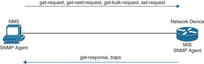
Figure 24-3 SNMP Communication Between NMS Host and Network Device
Now that the basic operations of SNMP have been listed, it is important to look at a MIB to understand some of the information or values that can be polled or send traps from SNMP. Example 24-29 shows some of the contents of the SNMPv2-MIB.my file. This file is publicly available on the Cisco website and shows what values can be polled in the MIB and to illustrate sending traps from SNMP.
Example 24-29 Partial Contents of SNMPv2-MIB.my
   -- the System group
   --
   -- a collection of objects common to all managed systems.

   system   OBJECT IDENTIFIER ::= { mib-2 1 }

   sysDescr OBJECT-TYPE
       SYNTAX      DisplayString (SIZE (0..255))
       MAX-ACCESS  read-only
       STATUS      current
       DESCRIPTION
               "A textual description of the entity.  This value should
               include the full name and version identification of
               the system's hardware type, software operating-system,
               and networking software."
       ::= { system 1 }

   sysObjectID OBJECT-TYPE
       SYNTAX      OBJECT IDENTIFIER
       MAX-ACCESS  read-only
       STATUS      current
       DESCRIPTION
               "The vendor's authoritative identification of the
               network management subsystem contained in the entity.
               This value is allocated within the SMI enterprises
               subtree (1.3.6.1.4.1) and provides an easy and
               unambiguous means for determining 'what kind of box' is
               being managed.  For example, if vendor 'Flintstones,
               Inc.' was assigned the subtree 1.3.6.1.4.1.424242,
               it could assign the identifier 1.3.6.1.4.1.424242.1.1
               to its 'Fred Router'."
       ::= { system 2 }

   sysUpTime OBJECT-TYPE
       SYNTAX      TimeTicks
       MAX-ACCESS  read-only
       STATUS      current
       DESCRIPTION
               "The time (in hundredths of a second) since the
               network management portion of the system was last
               re-initialized."
       ::= { system 3 }

   sysContact OBJECT-TYPE
       SYNTAX      DisplayString (SIZE (0..255))
       MAX-ACCESS  read-write
       STATUS      current
       DESCRIPTION
               "The textual identification of the contact person for
               this managed node, together with information on how
               to contact this person.  If no contact information is
               known, the value is the zero-length string."
       ::= { system 4 }

   sysName OBJECT-TYPE
       SYNTAX      DisplayString (SIZE (0..255))
       MAX-ACCESS  read-write
       STATUS      current
       DESCRIPTION
               "An administratively-assigned name for this managed
               node.  By convention, this is the node's fully-qualified
               domain name.  If the name is unknown, the value is
               the zero-length string."
       ::= { system 5 }

   sysLocation OBJECT-TYPE
       SYNTAX      DisplayString (SIZE (0..255))
       MAX-ACCESS  read-write
       STATUS      current
       DESCRIPTION
               "The physical location of this node (e.g., 'telephone
               closet, 3rd floor').  If the location is unknown, the
               value is the zero-length string."
       ::= { system 6 }
The structure of this MIB file is well documented and human readable. This portion of the file was selected to illustrate some of the portions of the MIB used in the configuration examples in this chapter as well as make it easier to tie back what is configured on a device to what it corresponds to inside a MIB file. Although configuring an NMS is not covered in this chapter, the device side that points to an NMS is covered in this section. The following list shows a handful of measures involved in setting up SNMP on a device to allow the device to be polled and send traps to an NMS:
Define the SNMP host or the NMS to send traps to.
Create an access list to restrict access via SNMP.
Define the read-only community string.
Define the read/write community string.
Define the SNMP location.
Define the SNMP contact.
These settings do not need to be configured in any particular order. However, it makes sense to configure the access list first and then the read-only and read/write strings. That way, when the device is accessible via SNMP, it is already locked down to only the allowed hosts within the access list. On R1, a standard access list is configured to only permit access from an NMS host on the 192.168.14.0/24 subnet. The host IP address is 192.168.14.100. Once the access list is configured, the read-only and read/write community strings are configured and bound to that access list. Example 24-30 illustrates this on R1. It is important to try to use SNMP strings that are not easy to guess from a security perspective.
Example 24-30 SNMP Access List on R1
R4(config)# access-list 99 permit 192.168.14.100 0.0.0.0
R4(config)# snmp-server community READONLY ro 99
R4(config)# snmp-server community READONLY rw 99
At this point, the device is configured to be polled from an NMS host with the IP address 192.168.14.100. If additional hosts need to be added, you simply add the new host IP addresses to the access list. It is also possible to permit the whole subnet. However, this is more of a security risk than specifying only the necessary hosts.
If a network operations team wants to send SNMP traps to an NMS, traps first must be enabled on the device. All available traps can be enabled by issuing the snmp-server enable traps command. However, this may enable unnecessary traps that have no significance to the network operations team. It might be more appropriate to be selective about which traps to enable. The traps that are available to be enabled is platform specific. A common approach to determining what traps are available is to look at the documentation for the device. It may be easier to simply issue the snmp-server enable traps command followed by ? to leverage the context-sensitive help and determine what traps are available on the device. Example 24-31 shows a partial list of traps that are available on R1.
Example 24-31 Available SNMP Traps on R1
R4(config)# snmp-server enable traps ?
  aaa_server       Enable SNMP AAA Server traps
  atm              Enable SNMP atm traps
  bfd              Allow SNMP BFD traps
  bgp              Enable BGP traps
  bstun            Enable SNMP BSTUN traps
  bulkstat         Enable Data-Collection-MIB Collection notifications
  ccme             Enable SNMP ccme traps
  cef              Enable SNMP CEF traps
  cnpd             Enable NBAR Protocol Discovery traps
  config           Enable SNMP config traps
  config-copy      Enable SNMP config-copy traps
  config-ctid      Enable SNMP config-ctid traps
  cpu              Allow cpu related traps
  dial             Enable SNMP dial control traps
  diameter         Allow Diameter related traps
  dlsw             Enable SNMP dlsw traps
  dnis             Enable SNMP DNIS traps
  ds1              Enable SNMP DS1 traps
  dsp              Enable SNMP dsp traps
  eigrp            Enable SNMP EIGRP traps
  entity           Enable SNMP entity traps
  entity-ext       Enable SNMP entity extension traps
 --More--
A significant number of traps can be enabled to send to an NMS. For the purpose of this section, the config trap will be enabled. In order to configure this trap, the snmp-server enable traps config command must be issued. Example 24-32 shows this command being used on R1 to enable the config trap to be sent to the NMS host at 192.168.14.100.
Example 24-32 Enabling SNMP Config Traps on R1
R4(config)# snmp-server enable traps config
R4(config)# snmp-server host 192.168.14.100 traps READONLY
syslog
Devices can generate a tremendous amount of useful information, including messages sent to the console, to the logging buffer, and to off-box syslog collectors. In fact, all three can be sent the same or different message types. This section briefly covers these options and provides a use case for each one. By default, all syslog messages are sent to the console. (This is how the debug commands from earlier in this chapter are displayed on the console port.) However, this can be adjusted, as can what messages are sent to the logging buffer or off-box syslog collector. It is critical to note that prior to configuring any device to send log information, the date and time of the clock must be properly configured for accurate time. If it is not, the time stamps on all the logging messages will not reflect the appropriate and accurate time, which will make troubleshooting much more difficult because you will not be able to correlate issues with the logs by using the time stamps generated. Ensuring that NTP is configured properly helps with this issue.
Messages that are generated have specific severity levels associated to them, but these levels can be changed. The default severity level of each message type is listed in Table 24-7.
Table 24-7 syslog Message Severity Levels
Level Keyword |
Level |
Description |
syslog Definition |
emergencies |
0 |
System unstable |
LOG_EMERG |
alerts |
1 |
Immediate action needed |
LOG_ALERT |
critical |
2 |
Critical conditions |
LOG_CRIT |
errors |
3 |
Error conditions |
LOG_ERR |
warnings |
4 |
Warning conditions |
LOG_WARNING |
notifications |
5 |
Normal but significant conditions |
LOG_NOTICE |
informational |
6 |
Informational messages only |
LOG_INFO |
debugging |
7 |
Debugging messages |
LOG_DEBUG |
These messages can be used to provide valuable information to the network operations staff, or they can be so overwhelming that they make it difficult to sift through to find or pinpoint an issue. It is important to note that having syslog configured doesn’t mean that an issue will be found. It still takes the proper skill to be able to look at the messages and determine the root cause of the issue. syslog is, however, very helpful in guiding you toward the issue at hand.
The logging buffer is the first area to focus on. On R1, you can enable logging to the buffer as follows:
Enable logging to the buffer.
Set the severity level of syslog messages to send to the buffer.
Set the logging buffer to a larger size.
The logging buffered ? command is issued from the global configuration mode to see the available options. Example 24-33 shows the list of available options. It is important to note that the severity level can be configured by simply specifying the level with a number from 0 to 7 or the name of the severity (listed next to the severity level number). The default size of the logging buffer is 4096 bytes. This can get overwritten quite quickly. It is good practice to expand the buffer size so you can capture more logging information.
Example 24-33 Logging the Buffer Severity Level on R1
R1(config)# logging buffered ?
  <0-7>              Logging severity level
  <4096-2147483647>  Logging buffer size
  alerts             Immediate action needed           (severity=1)
  critical           Critical conditions               (severity=2)
  debugging          Debugging messages                (severity=7)
  discriminator      Establish MD-Buffer association
  emergencies        System is unusable                (severity=0)
  errors             Error conditions                  (severity=3)
  filtered           Enable filtered logging
  informational      Informational messages            (severity=6)
  notifications      Normal but significant conditions (severity=5)
  warnings           Warning conditions                (severity=4)
  xml                Enable logging in XML to XML logging buffer
  <cr>
Debugging or severity 7 is the level that will be configured in this example; with this configuration, any debugging can be sent to the logging buffer instead of the console, which makes working on a device and troubleshooting less daunting as the debugging doesn’t interfere with the console output—that is, as long as the debugging level is not set on the console as well. In Example 24-34, the logging is configured to the debugging level, 7, and it is set to 100000 bytes. The do show logging command is then run to confirm the changes. Notice the syslog message that shows the logging size was changed.
Example 24-34 Configuring the Logging Buffer Size and Severity Level on R1
R1(config)# logging buffer 100000
R1(config)#
R1(config)# logging buffer debugging

R1(config)# do show logging
Syslog logging: enabled (0 messages dropped, 4 messages rate-limited, 0 flushes,
  0 overruns, xml disabled, filtering disabled)

No Active Message Discriminator.


No Inactive Message Discriminator.


    Console logging: disabled
    Monitor logging: level debugging, 0 messages logged, xml disabled,
                     filtering disabled
    Buffer logging:  level debugging, 1 messages logged, xml disabled,
                    filtering disabled
    Exception Logging: size (4096 bytes)
    Count and timestamp logging messages: disabled
    Persistent logging: disabled

No active filter modules.

    Trap logging: level informational, 108 message lines logged
        Logging Source-Interface:       VRF Name:

Log Buffer (100000 bytes):

*Jul 10 19:41:05.793: %SYS-5-LOG_CONFIG_CHANGE: Buffer logging: level debugging, xml
   disabled, filtering disabled, size (100000)
Now that the logging buffer has been configured for a severity level of debugging, it is good to show what happens when a debug command is used and stored in the buffer. Example 24-35 shows how to disable console logging and run debug ip ospf hello followed by the show logging command to reveal the debugging output on R1.
Example 24-35 Using the Logging Buffer on R1 for Debugging
R1(config)# no logging console
R1(config)# end
R1# debug ip ospf hello
OSPF hello debugging is on
R1# show logging
Syslog logging: enabled (0 messages dropped, 4 messages rate-limited, 0 flushes,
  0 overruns, xml disabled, filtering disabled)

No Active Message Discriminator.


No Inactive Message Discriminator.


    Console logging: disabled
    Monitor logging: level debugging, 0 messages logged, xml disabled,
                     filtering disabled
    Buffer logging:  level debugging, 11 messages logged, xml disabled,
                    filtering disabled
    Exception Logging: size (4096 bytes)
    Count and timestamp logging messages: disabled
    Persistent logging: disabled

No active filter modules.

    Trap logging: level informational, 109 message lines logged
        Logging Source-Interface:       VRF Name:

Log Buffer (100000 bytes):

*Jul 10 19:41:05.793: %SYS-5-LOG_CONFIG_CHANGE: Buffer logging: level debugging, xml
disabled, filtering disabled, size (100000)
*Jul 10 19:51:05.335: %SYS-5-CONFIG_I: Configured from console by console
*Jul 10 19:51:28.110: OSPF-1 HELLO Et0/0: Send hello to 224.0.0.5 area 0 from
  192.168.12.1
*Jul 10 19:51:30.923: OSPF-1 HELLO Et0/2: Send hello to 224.0.0.5 area 0 from
  192.168.17.1
*Jul 10 19:51:31.259: OSPF-1 HELLO Et0/2: Rcv hello from 7.7.7.7 area 0 192.168.17.7
*Jul 10 19:51:32.990: OSPF-1 HELLO Et0/0: Rcv hello from 2.2.2.2 area 0 192.168.12.2
*Jul 10 19:51:33.026: OSPF-1 HELLO Et0/1: Rcv hello from 4.4.4.4 area 0 192.168.14.4
*Jul 10 19:51:36.231: OSPF-1 HELLO Et0/1: Send hello to 224.0.0.5 area 0 from
  192.168.14.1
*Jul 10 19:51:37.376: OSPF-1 HELLO Et0/0: Send hello to 224.0.0.5 area 0 from
  192.168.12.1
*Jul 10 19:51:40.219: OSPF-1 HELLO Et0/2: Send hello to 224.0.0.5 area 0 from
  192.168.17.1
*Jul 10 19:51:40.706: OSPF-1 HELLO Et0/2: Rcv hello from 7.7.7.7 area 0 192.168.17.7
R1# undebug all
All possible debugging has been turned off
If a network operations team wanted to send these same logs to an off-box collector, that could be configured as well. By default, these messages are sent to the logging host through UDP port 514, but this can be changed if necessary. Configuring logging to a host is very similar to configuring logging on the console or buffer. In this case, it is configured by using the following steps:
Enable logging to host 192.168.14.100.
Set the severity level of syslog messages to send to host.
Example 24-36 shows the basic configuration for sending syslog messages to a collector or host from R1.
Example 24-36 Sending Logging to a Host on R1 for Debugging
R1(config)# logging host 192.168.14.100
R1(config)# logging trap 7
R1(config)# do show logging
Syslog logging: enabled (0 messages dropped, 4 messages rate-limited, 0 flushes,
  0 overruns, xml disabled, filtering disabled)

No Active Message Discriminator.


No Inactive Message Discriminator.


    Console logging: disabled
    Monitor logging: level debugging, 0 messages logged, xml disabled,
                     filtering disabled
    Buffer logging:  level debugging, 22 messages logged, xml disabled,
                    filtering disabled
    Exception Logging: size (4096 bytes)
    Count and timestamp logging messages: disabled
    Persistent logging: disabled

No active filter modules.

    Trap logging: level debugging, 112 message lines logged
        Logging to 192.168.14.100  (udp port 514, audit disabled,
              link up),
              1 message lines logged,
              0 message lines rate-limited,
              0 message lines dropped-by-MD,
              xml disabled, sequence number disabled
              filtering disabled
The power of using syslog is evident even in these basic examples. It can be used to notify of power supply failures, CPU spikes, and a variety of other things. It is important not to underestimate the level of granularity and detail that can be achieved by setting up proper notification policies in a network. This section provides a high-level discussion on the topic, but it is easy to go extremely deep on the subject. It is ultimately up to the network operations team to determine how deep is appropriate to meet the business’s needs. There are many options available, such as multiple logging destinations and ways to systematically set up different levels of logging. It all depends on what the network operations team feels is appropriate for their environment.
NetFlow and Flexible NetFlow
Gathering statistics about a network during its operations is not only useful but important. Gathering statistical information on traffic flows is necessary for a number of reasons. Some businesses, such as service providers, use it for customer billing. Other businesses use it to determine whether traffic is optimally flowing through the network. Some use it for troubleshooting if the network is not performing correctly. NetFlow is very versatile and provides a wealth of information without much configuration burden. That being said, NetFlow has two components that must be configured: NetFlow Data Capture and NetFlow Data Export. NetFlow Data Capture captures the traffic statistics. NetFlow Data Export exports the statistical data to a NetFlow collector, such as Cisco DNA Center or Cisco Prime Infrastructure. Examples of each of these are provided in this section.
There are a couple things to note from a design perspective prior to enabling NetFlow. First, NetFlow consumes memory resources. The traffic statistics are captured in the memory cache. The default size of the cache is platform specific and should be investigated prior to enabling NetFlow. This is especially the case with older platforms that potentially have lower memory resources available.
NetFlow captures traffic on ingress and egress—that is, traffic that is coming into the devices as well as traffic that is leaving them. Table 24-8 lists the different types of ingress and egress traffic collected with NetFlow Version 9 on a Cisco IOS device.
Table 24-8 NetFlow Ingress and Egress Collected Traffic Types
Ingress |
Egress |
IP to IP packets |
NetFlow accounting for all IP traffic packets |
IP to Multiprotocol Label Switching (MPLS) packets |
MPLS to IP packets |
Frame Relay terminated packets |
|
ATM terminated packets |
|
NetFlow collects traffic based on flows. A flow is a unidirectional traffic stream that contains a combination of the following key fields:
Source IP address
Destination IP address
Source port number
Destination port number
Layer 3 protocol type
Type of service (ToS)
Input logical interface
The following example shows how to enable NetFlow on a device. (If the desired intention is not to export the NetFlow data to a collector, that step can be skipped.) This example covers configuring R1’s Ethernet0/1 interface for NetFlow Data Capture and exporting the data to the 192.168.14.100 collector. The steps are rather simple. Example 24-37 illustrates the process of configuring NetFlow Data Capture and NetFlow Data Export on R1.
Example 24-37 Configuring NetFlow and NetFlow Data Export on R1
R1# configure terminal
Enter configuration commands, one per line.  End with CNTL/Z.
R1(config)# ip flow-export version 9
R1(config)# ip flow-export destination 192.168.14.100 9999
R1(config)# interface Ethernet0/1
R1(config-if)# ip flow ingress
R1(config-if)# ip flow egress
R1(config-if)# end
R1#
To verify that NetFlow and NetFlow Data Export were configured properly, a few commands can be run from the command-line interface. The first is show ip flow interface, which shows the interfaces that are configured for NetFlow. The second is the show ip flow export command, which shows the destination for the NetFlow data to be exported to as well as statistics on the export, including any errors that may arise. Finally, the show ip cache flow command shows the traffic flows that NetFlow is capturing. Example 24-38 shows the output of these three commands.
Example 24-38 Verifying NetFlow and NetFlow Data Export Configuration on R1
R1# show ip flow interface
Ethernet0/1
  ip flow ingress
  ip flow egress
R1#
R1# show ip flow export
Flow export v9 is enabled for main cache
  Export source and destination details :
  VRF ID : Default
    Destination(1)  192.168.14.100 (9999)
  Version 9 flow records
  0 flows exported in 0 udp datagrams
  0 flows failed due to lack of export packet
  0 export packets were sent up to process level
  0 export packets were dropped due to no fib
  0 export packets were dropped due to adjacency issues
  0 export packets were dropped due to fragmentation failures
  0 export packets were dropped due to encapsulation fixup failures
R1# show ip cache flow
IP packet size distribution (6 total packets):
   1-32   64   96  128  160  192  224  256  288  320  352  384  416  448  480
   .000 .666 .333 .000 .000 .000 .000 .000 .000 .000 .000 .000 .000 .000 .000

    512  544  576 1024 1536 2048 2560 3072 3584 4096 4608
   .000 .000 .000 .000 .000 .000 .000 .000 .000 .000 .000

IP Flow Switching Cache, 278544 bytes
  2 active, 4094 inactive, 2 added
  29 ager polls, 0 flow alloc failures
  Active flows timeout in 30 minutes
  Inactive flows timeout in 15 seconds
IP Sub Flow Cache, 34056 bytes
  2 active, 1022 inactive, 2 added, 2 added to flow
  0 alloc failures, 0 force free
  1 chunk, 1 chunk added
  last clearing of statistics never
Protocol         Total    Flows   Packets Bytes  Packets Active(Sec) Idle(Sec)
--------         Flows     /Sec     /Flow  /Pkt     /Sec     /Flow     /Flow

SrcIf         SrcIPaddress    DstIf         DstIPaddress    Pr SrcP DstP  Pkts
Et0/1         192.168.14.4    Null          224.0.0.5       59 0000 0000     2

SrcIf         SrcIPaddress    DstIf         DstIPaddress    Pr SrcP DstP  Pkts
Et0/1         192.168.14.4    Null          224.0.0.2       11 0286 0286     4
Another great option for NetFlow is being able to configure the top specified number of talkers on the network. A very useful and quick configuration allows you to gain a great snapshot of what is going on in a device from a flow perspective. This view can be enabled by issuing the global configuration mode command ip flow-top-talkers and configuring the top command for the number of talkers (1–200) and the sort-by command to sort by bytes or packets, depending on the use case. Example 24-39 shows the configuration steps on R1 and the associated verification steps.
Example 24-39 Configuring and Verifying the Top Talkers on R1
R1# configure terminal
Enter configuration commands, one per line.  End with CNTL/Z.
R1(config)# ip flow-top-talkers
R1(config-flow-top-talkers)# top 10
R1(config-flow-top-talkers)# sort-by bytes
R1(config-flow-top-talkers)# end
R1#
R1#
R1# show ip flow top-talkers

SrcIf         SrcIPaddress    DstIf         DstIPaddress    Pr SrcP DstP Bytes
Et0/1         192.168.14.4    Null          224.0.0.2       11 0286 0286  9610
Et0/1         192.168.14.4    Null          224.0.0.5       59 0000 0000  5820
2 of 10 top talkers shown. 2 of 2 flows matched.

R1#
Flexible NetFlow was created to aid in more complex traffic analysis configuration than is possible with traditional NetFlow. Flexible NetFlow allows for the use and reuse of configuration components. Table 24-9 lists the components that make Flexible NetFlow powerful. Flexible NetFlow allows for the use of multiple flow monitors on the same traffic at the same time. This means that multiple different flow policies can be applied to the same traffic as it flows through a device. If two different departments have a reason to analyze the traffic, they can both do so by using different parameters in each flow monitor.
Table 24-9 Flexible NetFlow Components
Component Name |
Description |
Flow Records |
Combination of key and non-key fields. There are predefined and user-defined records. |
Flow Monitors |
Applied to the interface to perform network traffic monitoring. |
Flow Exporters |
Exports NetFlow Version 9 data from the Flow Monitor cache to a remote host or NetFlow collector. |
Flow Samplers |
Samples partial NetFlow data rather than analyzing all NetFlow data. |
There are trade-offs in using sampled NetFlow data. The biggest one is that there is a reduced load on the device in terms of memory and CPU. However, by sampling NetFlow data only at specific intervals, something could be missed as the accuracy goes down with sampling compared to when gathering all data. Depending on the use case and the environment, however, sampling may be perfectly acceptable. It all depends on the business and its priorities.
Security has been a huge driver in the adoption of Flexible NetFlow due to its ability to track all parts of the IP header as well as the packet and normalize it into flows. Flexible NetFlow can dynamically create individual caches for each type of flow. In addition, Flexible NetFlow can filter ingress traffic destined to a single destination. These factors make Flexible NetFlow a very powerful security asset.
You can use the collect and match commands to create a customized flow record. To create a custom flow record, certain key and non-key fields must be matched so the flow record is usable. The match command is used to select key fields, and the collect command is used to select non-key fields. Table 24-10 shows a list of the key and non-key fields that can be used to mimic the original NetFlow capabilities when building a custom flow record.
Table 24-10 Flow Record Key and Non-Key Fields
Field |
Key or Non-Key Field |
Definition |
IP ToS |
Key |
Value in the type of service (ToS) field |
IP protocol |
Key |
Value in the IP protocol field |
IP source address |
Key |
IP source address |
IP destination address |
Key |
IP destination address |
Transport source port |
Key |
Value of the transport layer source port field |
Transport destination port |
Key |
Value of the transport layer destination port field |
Interface input |
Key |
Interface on which the traffic is received |
Flow sampler ID |
Key |
ID number of the flow sampler (if flow sampling is enabled) |
IP source AS |
Non-key |
Source autonomous system number |
IP destination AS |
Non-key |
Destination autonomous system number |
IP next-hop address |
Non-key |
IP address of the next hop |
IP source mask |
Non-key |
Mask for the IP source address |
IP destination mask |
Non-key |
Mask for the IP destination address |
TCP flags |
Non-key |
Value in the TCP flag field |
Interface output |
Non-key |
Interface on which the traffic is transmitted |
Counter bytes |
Non-key |
Number of bytes seen in the flow |
Counter packets |
Non-key |
Number of packets seen in the flow |
Time stamp system uptime first |
Non-key |
System uptime (time, in milliseconds, since this device was first booted) when the first packet was switched |
Time stamp system uptime last |
Non-key |
System uptime (time, in milliseconds, since this device was first booted) when the last packet was switched |
Configuring flow records is an important step in enabling Flexible NetFlow because the flow record defines what type of traffic will be analyzed or monitored. There are predefined flow records, and you can also create custom flow records. Custom flow records can have hundreds of different combinations to meet the exact needs of the business. Configuring a custom flow record involves the following steps:
Define the flow record name.
Set a useful description of the flow record.
Set match criteria for key fields.
Define non-key fields to be collected.
Although many of the predefined flow records that are available may be suitable for many use cases, there are too many of them to cover here. Having the ability to build a custom flow record for a specific and unique use case makes it extremely powerful. Example 24-40 shows a custom flow record called CUSTOM1 being defined on R4. This example uses the match command to match the IPv4 destination address and the collect command to gather the byte and packet counts. To verify the flow record configuration, the command show flow record CUSTOM1 can be used. To see all flow records configured, including predefined flow records, the show flow record command by itself can be used. The show run flow record command also shows the running configuration of the customer flow records that were created.
Example 24-40 Configuring and Verifying the Custom Flow Record on R4
R4# configure terminal
Enter configuration commands, one per line.  End with CNTL/Z.
R4(config)# flow record CUSTOM1
R4(config-flow-record)# description Custom Flow Record for IPv4 Traffic
R4(config-flow-record)# match ipv4 destination address
R4(config-flow-record)# collect counter bytes
R4(config-flow-record)# collect counter packets
R4(config-flow-record)# exit
R4(config)#
R4(config)# do show flow record CUSTOM1
flow record CUSTOM1:
  Description:        Custom Flow Record for IPv4 Traffic
  No. of users:       0
  Total field space:  12 bytes
  Fields:
    match ipv4 destination address
    collect counter bytes
    collect counter packets

R4(config)#
R4(config)#do show running-config flow record
Current configuration:
!
flow record CUSTOM1
 description Custom Flow Record for IPv4 Traffic
 match ipv4 destination address
 collect counter bytes
 collect counter packets
!
R4(config)#
Now that a custom flow record has been configured, the flow exporter can be created. There are a few important steps to complete when building a flow exporter:
Define the flow exporter name.
Set a useful description of the flow exporter.
Specify the destination of the flow exporter to be used.
Specify NetFlow version to export.
Specify the UDP port.
In this instance, the exporter that will be created will point to the 192.168.14.100 host that has been used in other examples in this chapter. This step in the process exports flow data from the device to a NetFlow collector or management platform such as Cisco DNA Center or Cisco Prime Infrastructure. Example 24-41 illustrates the configuration of the flow exporter as well as how to verify the configuration on R4.
Example 24-41 Configuring and Verifying the Custom Flow Exporter on R4
R4# configure terminal
Enter configuration commands, one per line.  End with CNTL/Z.
R4(config)# flow exporter CUSTOM1
R4(config-flow-exporter)# description EXPORT-TO-NETFLOW-COLLECTOR
R4(config-flow-exporter)# destination 192.168.14.100
R4(config-flow-exporter)# export-protocol netflow-v9
R4(config-flow-exporter)# transport UDP 9999
R4(config-flow-exporter)# exit
R4(config)# exit
R4# sh run flow exporter
Current configuration:
!
flow exporter CUSTOM1
 description EXPORT-TO-NETFLOW-COLLECTOR
 destination 192.168.14.100
 transport udp 9999
!
R4#
R4# show flow exporter CUSTOM1
Flow Exporter CUSTOM1:
  Description:              EXPORT-TO-NETFLOW-COLLECTOR
  Export protocol:          NetFlow Version 9
  Transport Configuration:
    Destination IP address: 192.168.14.100
    Source IP address:      192.168.14.4
    Transport Protocol:     UDP
    Destination Port:       9999
    Source Port:            50192
    DSCP:                   0x0
    TTL:                    255
    Output Features:        Not Used
R4#
Now that a custom flow exporter called CUSTOM1 has been configured, the flow monitor must be created. Each flow monitor requires a flow record to be assigned to it. Each flow monitor has its own cache, and the flow record provides the layout and how to carve up the cache for the defined traffic defined in the flow record. The flow monitor can use the predefined flow records or custom flow records. For the purpose of this section, the CUSTOM1 flow record is used to illustrate the configuration steps. To configure a flow monitor, the following high-level steps must be taken:
Define the flow monitor name.
Set a useful description of the flow monitor.
Specify the flow record to be used.
Specify a cache timeout of 60 for active connections.
Assign the exporter to the monitor.
Configuring a flow monitor is a pretty straightforward task. The cache timeout tells the device to export the cache to the collector every 60 seconds. It is important when creating a flow monitor for the description of the flow monitor to be useful and to map back to the flow record. Similarly, when configuring QoS, it is nice to have the descriptions self-document the intent of what the policy is doing. This helps when configuring the flow monitor and when using context sensitive help, as the description that is configured shows in the output. Example 24-42 shows this as well as the configuration and verification for the flow monitor called CUSTOM1.
Example 24-42 Configuring and Verifying the Custom Flow Monitor on R4
R4(config)# flow monitor CUSTOM1
R4(config-flow-monitor)# description Uses Custom Flow Record CUSTOM1 for IPv4$
R4(config-flow-monitor)# record ?
  CUSTOM1           Custom Flow Record for IPv4 Traffic
  netflow           Traditional NetFlow collection schemes
  netflow-original  Traditional IPv4 input NetFlow with origin ASs
R4(config-flow-monitor)# record CUSTOM1
R4(config-flow-monitor)# cache active timeout 60
R4(config-flow-monitor)# end
R4# show run flow monitor CUSTOM1
Current configuration:
!
flow monitor CUSTOM1
 description Uses Custom Flow Record CUSTOM1 for IPv4 Traffic
 cache timeout active 60
 record CUSTOM1
!
R4# show flow monitor CUSTOM1
Flow Monitor CUSTOM1:
  Description:       Uses Custom Flow Record CUSTOM1 for IPv4 Traffic
  Flow Record:       CUSTOM1
  Cache:
    Type:                 normal
    Status:               not allocated
    Size:                 4096 entries / 0 bytes
    Inactive Timeout:     15 secs
    Active Timeout:       60 secs
    Update Timeout:       1800 secs
    Synchronized Timeout: 600 secs
R4#
The next step is to map the flow exporter CUSTOM1 to the flow monitor CUSTOM1. You need to essentially map the two together so the traffic that is being collected by the flow record can be exported to the NetFlow collector at 192.168.14.100. Example 24-43 shows the process and verification for adding the flow exporter CUSTOM1 to the flow monitor CUSTOM1 on R4. The output illustrates the need for clear and detailed descriptions throughout the process.
Example 24-43 Configuring and Verifying the Flow Exporter Mapping to the Flow Monitor on R4
R4# configure terminal
Enter configuration commands, one per line.  End with CNTL/Z.
R4(config)# flow monitor CUSTOM1
R4(config-flow-monitor)# exporter ?
 CUSTOM1  EXPORT-TO-NETFLOW-COLLECTOR
R4(config-flow-monitor)# exporter CUSTOM1
R4(config-flow-monitor)# end
R4# show run flow monitor
Current configuration:
!
flow monitor CUSTOM1
 description Uses Custom Flow Record CUSTOM1 for IPv4 Traffic
 exporter CUSTOM1
 cache timeout active 60
 record CUSTOM1
!
R4# show flow monitor CUSTOM1
Flow Monitor CUSTOM1:
  Description:       Uses Custom Flow Record CUSTOM1 for IPv4 Traffic
  Flow Record:       CUSTOM1
  Flow Exporter:     CUSTOM1 (inactive)
  Cache:
    Type:                 normal
    Status:               not allocated
    Size:                 4096 entries / 0 bytes
    Inactive Timeout:     15 secs
    Active Timeout:       60 secs
    Update Timeout:       1800 secs
    Synchronized Timeout: 600 secs
R4#
The final step necessary in enabling Flexible NetFlow is to apply the flow monitor to the interfaces. This step turns on the collection of NetFlow statistics, and it can be enabled for ingress or egress or both. This scenario highlights the ingress option, using the ip flow monitor CUSTOM1 input command on the desired interfaces. Example 24-44 illustrates the process as well as how to verify that Flexible NetFlow is working by issuing the show ip flow monitor CUSTOM1 cache command.
Example 24-44 Configuring and Verifying the Flow Monitor Interface Commands on R4
R4(config)# interface ethernet0/1
R4(config-if)# ip flow monitor ?
  CUSTOM1         Uses Custom Flow Record CUSTOM1 for IPv4 Traffic
R4(config-if)# ip flow monitor CUSTOM1 input
R4(config-if)# interface ethernet0/2
R4(config-if)# ip flow monitor CUSTOM1 input
R4(config-if)# end
R4# show flow monitor CUSTOM1 cache
  Cache type:                               Normal
  Cache size:                                 4096
  Current entries:                               3
  High Watermark:                                3

  Flows added:                                   8
  Flows aged:                                    5
    - Active timeout      (    60 secs)          5
    - Inactive timeout    (    15 secs)          0
    - Event aged                                 0
    - Watermark aged                             0
    - Emergency aged                             0

IPV4 DST ADDR         bytes        pkts
===============  ==========  ==========
224.0.0.5               560           7
224.0.0.2               372           6
4.4.4.4                 674          11
The modularity of Flexible NetFlow makes the tool much more scalable and powerful than traditional NetFlow. Having the ability to export to multiple destinations or collectors as well as having the capability of using the tool for security forensics to identify DoS attacks and worm propagation is tremendous. Although there are quite a few steps involved in enabling Flexible NetFlow, the process is easily replicable, so network engineers can easily create traffic analysis to meet the individual needs of the business or multiple departments within the same organization.
Switched Port Analyzer (SPAN) Technologies
The famous saying about “three sides to every story” holds true when troubleshooting network-based issues, where there are the perspectives of the local device, the remote device, and what is transmitted on the wire. Regardless of whether one device is a router, a firewall, a load balancer, or a computer, there are often tools that allow for troubleshooting processes locally on the device. Understanding what was transmitted on the wire can help pinpoint problems.
Gaining the perspective of what happens on the wire can be more complicated. When the problem appears to be a Layer 2 issue, there are a few options:
Insert a splitter between the devices. Splitters are generally applicable to optical connections as they split the light across a prism. The original source stays intact, and a second stream can be sent to a traffic analyzer.
Configure the network device to mirror the packets at the data plane level to an additional destination. The destination can be a local port or a remote port that is connected to a traffic analyzer.
Insert a switch between the two devices and then configure the switch to mirror the transient traffic to a traffic analyzer.
Catalyst switches provide the Switched Port Analyzer (SPAN), which makes it possible to capture packets using the second two options above by using the following techniques:
Local Switched Port Analyzer: You can capture local network traffic on a switch and send a copy of the network traffic to a local port attached to some sort of traffic analyzer.
Remote Switched Port Analyzer (RSPAN): You can capture network traffic on a remote switch and send a copy of the network traffic to the local switch through Layer 2 (switching) toward a local port attached to some sort of traffic analyzer.
Encapsulated Remote Switched Port Analyzer (ERSPAN): You can capture network traffic on a remote device and send the traffic to the local system through Layer 3 (routing) toward a local port attached to some sort of traffic analyzer.
Figure 24-4 shows a sample topology with four computers (PC-A, PC-B, PC-C, and PC-D) spread across three switches and a traffic analyzer connected to SW1. PC-A, PC-B, and PC-C are all connected to VLAN 123 on the 10.123.1.0/24 network, and PC-D is connected to VLAN 34, which is on the 10.34.1.0/24 network. This topology is used to demonstrate the concepts of SPAN, RSPAN, and ERSPAN.
Figure 24-4 Sample Topology for Packet Captures
Local SPAN
A local SPAN session is the most basic form of packet capture as all the configuration occurs on a single switch. The destination of the mirrored traffic can be one or more local ports. The source of the packet capture can be only one of the following:
One or more specific switch ports
A port channel (also known as an EtherChannel)
A VLAN (To be more explicit, this is the traffic received by the switch for hosts all the hosts associated to the VLAN specified. This does not include a SVI interface.)
Also consider the following:
Most switches support at least two SPAN sessions, but newer hardware can support more than two sessions.
The source port cannot be reused between two different SPAN sessions.
Source ports can be switched or routed ports.
The destination cannot be reused between two different SPAN sessions.
It is possible to saturate the destination port if the source ports are receiving more data than the destination port can transmit. In other words, if the source ports are 10Gigabit ports and the destination port is just Gigabit, it is possible that packet loss will occur on the destination port.
Specifying the Source Ports
The source ports are defined with the global configuration command monitor session session-id source {interface interface-id | vlan vlan-id} [rx | tx | both]. The SPAN session-id allows for the switch to correlate the source ports to specific destination ports. One or more interfaces or VLANs can be entered by using either a comma (for delimiting multiple interfaces) or a hyphen (for setting a range). Another option is to repeat the command with a different value and let the system update the source range accordingly.
The direction of the traffic can be specified as part of the configuration. With the optional rx keyword you capture only traffic received on that source, with the optional tx keyword you capture traffic sent by that source, and with the both keyword you capture all traffic. By default, traffic is captured for both.
You can specify a trunk port as a source port to capture traffic for all VLANs that traverse that port. This might provide too much data and add noise to the traffic analysis tool. The VLANs can be filtered on the capture with the command monitor session session-id filter vlan vlan-range.
Specifying the Destination Ports
The destination port is specified with the global configuration command:
monitor session session-id destination interface interface-id [encapsulation
  {dot1q [ingress {dot1q vlan vlan-id | untagged vlan vlan-id | vlan vlan-id}|
  replicate [ingress {dot1q vlan vlan-id | untagged vlan vlan-id]}} | ingress]
As you can see, there are a lot of different nested options.
A SPAN session normally copies the packets without including any 802.1Q VLAN tags or Layer 2 protocols, like Spanning Tree Protocol (STP) bridge protocol data units (BPDUs), CDP, VTP, DTP, Port Aggregation Protocol (PAgP), or Link Aggregation Control Protocol (LACP). Using the encapsulation replicate keywords includes that information. The full global configuration command is:
monitor session session-id destination interface interface-id [encapsulation
  replicate]
Normally, the SPAN destination port only receives traffic and drops ingress traffic. However, in some scenarios, connectivity to the traffic analyzer might be required. For example, if the traffic analyzer is a Windows PC and is accessed using RDP, the port must be able to send and receive traffic for the Windows PC in addition to the traffic from the SPAN session. Situations like this require the following global configuration command:
monitor session session-id destination interface interface-id ingress {dot1q vlan
  vlan-id | untagged vlan vlan-id}
Selecting the dot1q keyword requires the packets to be encapsulated with the specified VLAN ID. Selecting the untagged keyword accepts incoming packets and associates them to the specified VLAN ID.
These commands might seem confusing, but the following section illustrates a couple scenarios (using Figure 24-4) and provides the associated configurations to help clarify the commands.
Local SPAN Configuration Examples
Example 24-45 shows how to monitor both PC-A’s and PC-B’s communication on SW1 and send it toward the local traffic analyzer.
Example 24-45 Enabling a SPAN Session on SW1
SW1(config)# monitor session 1 source interface gi1/0/1 - 2
SW1(config)# monitor session 1 destination interface gi1/0/9
The session information can be viewed with the command show monitor session {session-id [detail] | local [detail]}. A specific SPAN session can be viewed, or the output can be restricted to the local SPAN session, as shown in Example 24-46.
Example 24-46 Verifying the Configured SPAN Session
SW1# show monitor session local
Session 1
---------
Type                     : Local Session
Source Ports             :
    Both                 : Gi1/0/1-2
Destination Ports        : Gi1/0/9
    Encapsulation        : Native
          Ingress        : Disabled
The next example illustrates monitoring the trunk port Gi1/0/10 and provides the output to PC-B for PC-A and PC-B communication on SW1 and sending it toward the local traffic analyzer. The source port is a trunk port, and it is important to restrict traffic to VLAN 123 and capture Layer 2 QoS markings.
Example 24-47 shows the commands that are entered on SW1 and then shows the configuration verified by examining the SPAN session.
Example 24-47 Configuring and Verifying SPAN for the SW1 Gi1/0/10 Source
SW1(config)# monitor session 1 source interface gi1/0/10
! Some of the following command keywords were shortened for autocomplete
! so they all appear on the same line.
SW1(config)# monitor session 1 destination interface Gi1/0/9 encapsulation replicate
SW1(config)# monitor session 1 filter vlan 123
SW1# show monitor session 1
Session 1
---------
Type                     : Local Session
Source Ports             :
    Both                 : Gi1/0/10
Destination Ports        : Gi1/0/9
    Encapsulation        : Replicate
          Ingress        : Disabled
Filter VLANs             : 123
In the last scenario, the switch is configured to monitor PC-A’s traffic, and it uses an already installed network traffic analysis tool on PC-B. When the switch is configured, PC-B can be accessed remotely to view the network traffic by using RDP. Example 24-48 lists the commands that are entered on SW1 to capture the ingress traffic and shows the configuration being verified.
Example 24-48 Configuring and Verifying SPAN for the SW1 Gi1/0/1 Source
SW1(config)# monitor session 1 source interface gi1/0/1
! Some of the following command keywords were shortened for autocomplete
! so they all appear on the same line.
SW1(config)# monitor session 1 destination interface gi1/0/2 ingress untagged vlan
123
SW1# show monitor session 1
Session 1
---------
Type                     : Local Session
Source Ports             :
    Both                 : Gi1/0/1
Destination Ports        : Gi1/0/2
    Encapsulation        : Native
          Ingress        : Enabled, default VLAN = 123
    Ingress encap        : Untagged
Remote SPAN (RSPAN)
In large environments, it might be not be possible to move a network analyzer to other parts of the network. The RSPAN function allows the source ports to be located on one switch and the destination port on a different switch. The mirror traffic is placed on a special VLAN called the RSPAN VLAN, which is designated for SPAN traffic only.
A switch with the RSPAN VLAN operates differently from a typical switch:
MAC addresses are not learned on ports associated with the RSPAN VLAN. This ensures that the switch does not try to use the port associated with the RSPAN VLAN to transmit data to the end host, which in turn ensures that the normal forwarding path is maintained.
Traffic is flooded out all the ports associated to the RSPAN VLAN. The RSPAN VLAN should not be associated with ports that are not trunk ports between the source and destination switches.
The configuration for RSPAN is straightforward: A VLAN is created and then identified as an RSPAN VLAN with the command remote-span. The VLAN needs to be the same on all switches for that RSPAN session. Example 24-49 shows the RSPAN VLAN being created on SW1 and SW2.
Example 24-49 Creating the RSPAN VLAN
SW1(config)# vlan 99
SW1(config-vlan)# name RSPAN_VLAN
SW1(config-vlan)# remote-span
SW2(config)# vlan 99
SW2(config-vlan)# name RSPAN_VLAN
SW2(config-vlan)# remote-span
On the source port switch, the source ports are selected just as explained earlier for local SPAN. However, the destination is the RSPAN VLAN, which is set with the command monitor session session-id destination remote vlan rspanvlan-id. While the session-id is locally significant, keeping it the same on both the source and destination switches prevents confusion.
Example 24-50 shows the configuration of RSPAN on the source switch, SW2. Traffic from PC-C is sent to SW1 for analysis.
Example 24-50 Configuring a Source RSPAN Switch
SW2(config)# monitor session 1 source interface gi1/0/3
SW2(config)# monitor session 1 destination remote vlan 99
On the destination port switch, the destination ports are selected just as explained earlier for local SPAN. However, the source is the RSPAN VLAN, and this is set with the command monitor session session-id source remote vlan rspanvlan-id. While the session-id is locally significant, keeping it the same on both the source and destination switches prevents confusion.
Example 24-51 shows the configuration of RSPAN on the destination switch, SW1. The traffic is sent to the traffic analyzer for analysis.
Example 24-51 Configuring a Destination RSPAN Switch
SW1(config)# monitor session 1 source remote vlan 99
SW1(config)# monitor session 1 destination interface gi1/0/9
Example 24-52 verifies the configuration of RSPAN on both SW1 and SW2.
Example 24-52 Verifying the RSPAN Settings
SW1# show monitor session 1
Session 1
---------
Type                     : Remote Destination Session
Source RSPAN VLAN        : 99
Destination Ports        : Gi1/0/9
    Encapsulation        : Native
          Ingress        : Disabled
SW2# show monitor session remote
Session 1
---------
Type                     : Remote Source Session
Source Ports             :
    Both                 : Gi1/0/3
Dest RSPAN VLAN          : 99
Just as with a local SPAN session, traffic is duplicated with an RSPAN. This is significant in that additional traffic must traverse the trunk link and could starve out normal network traffic. Because a trunk link is used to carry the RSPAN VLAN, STP operates on the RSPAN VLAN, and STP BPDUs cannot be filtered as filtering could introduce a forwarding loop.
Encapsulated Remote SPAN (ERSPAN)
In large environments, it might not be possible to move a network analyzer to other parts of the network. ERSPAN provides the ability to monitor traffic in one area of the network and route the SPAN traffic to a traffic analyzer in another area of the network through Layer 3 routing. Think of a large-scale WAN with multiple remote sites and being able to do packet captures from anywhere that has IP connectivity. That is a powerful use case for ERSPAN. The configuration commands are similar in nature to those for SPAN and RSPAN. However, because the traffic is routed to another portion of the network, some additional configuration settings must take place to enable this capability.
Specifying the Source Ports
A source and destination must be configured. To configure a source, the following command is issued: monitor session span-session-number type erspan-source. This defines the session number as well as the session type, erspan-source. Equally important as configuring the session is setting a useful description to document the purpose of the ERSPAN session. The description description command can be used for this purpose.
Once the initial session is created, the source must be defined in the session. This is accomplished by issuing the source { interface type number | vlan vlan-ID } [ , | - | both | rx | tx ] command. As mentioned earlier in this chapter, if the source is a trunk port, it is important to filter based on the specific VLAN to be used as a source. This can be done using the filter { ip { standard-access-list | expanded-access-list | acl-name } | ipv6 { access-group acl-name } | vlan vlan-ID } command. This example does not use a trunk link as a source interface.
When all these settings have been configured, the session must be enabled with the no shutdown command to ensure that the session is active.
Specifying the Destination
When the source has been configured, it is necessary to configure the destination of the ERSPAN session. To enter the destination subconfiguration mode, the destination command is used. The rest of the commands will be issued in the destination subconfiguration mode to specify the destination of the ERSPAN session as well as any parameters associated with the configuration of the destination.
The next step is to identify the IP address of the destination for the ERSPAN session. Because this is a Layer 3 SPAN session, this IP address is where the traffic will be sent to be analyzed. The command to configure this action is simply ip address ip-address. Much like the source session, the destination session must have a unique identifier. This is configured with the erspan-id erspan-ID command. Once this is configured, the source IP address or origin of the ERSPAN traffic must be specified. This is achieved by issuing the origin ip address ip-address command.
The final step is to assign a ToS or TTL to the ERSPAN traffic. This is done with the erspan { tos tos-value | ttl ttl-value } command from global configuration mode. This example shows the ttl option being set. Example 24-53 illustrates this whole process. In addition, to verify the configured sessions, the show monitor session erspan-source session is issued on SW1.
Example 24-53 Configuring ERSPAN on SW1
SW4# configure terminal
SW4(config)# monitor session 1 type erspan-source
SW4(config-mon-erspan-src)# description SOURCE-PC-D-TRAFFIC
SW4(config-mon-erspan-src)# source interface GigabitEthernet 1/0/4 rx
SW4(config-mon-erspan-src)# filter vlan 34
SW4(config-mon-erspan-src)# no shutdown
SW4(config-mon-erspan-src)# destination
SW4(config-mon-erspan-src-dst)# ip address 10.123.1.100
SW4(config-mon-erspan-src-dst)# erspan-id 2
SW4(config-mon-erspan-src-dst)# origin ip address 10.34.1.4
SW4(config-mon-erspan-src)# exit
SW4(config)# erspan ttl 32
SW4(config)# end
SW4#
SW4# show monitor session erspan-source session

Type : ERSPAN Source Session
Status : Admin Enabled
Source Ports :
RX Only : Gi1/0/4
Destination IP Address : 10.123.1.100
Destination ERSPAN ID : 2
Origin IP Address : 10.34.1.4
IPv6 Flow Label : None
IP SLA
IP SLA is a tool built into Cisco IOS software that allows for the continuous monitoring of various aspects of the network. The different types of probes that can be configured to monitor traffic within a network environment include the following:
Delay (both round-trip and one-way)
Jitter (directional)
Packet loss (directional)
Packet sequencing (packet ordering)
Path (per hop)
Connectivity (directional)
Server or website download time
Voice quality scores
IP SLA has proven to be a very useful tool as it provides a variety of flexible monitoring options. Typically, any SLA received from a service provider only monitors or guarantees the traffic as it flows across the service provider’s network. This doesn’t provide an end-to-end SLA—or visibility, for that matter. However, IP SLA is a robust tool that can help with troubleshooting. Figure 24-5 shows this scenario and illustrates why IP SLA provides more visibility that a typical service provider SLA.
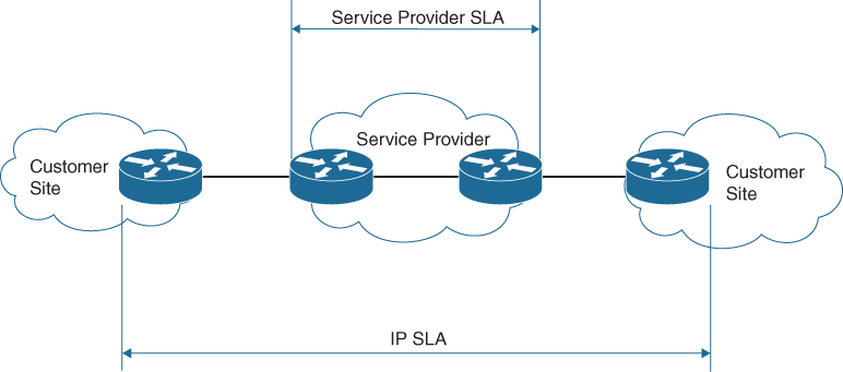
Figure 24-5 IP SLA and Typical Service Provider SLA
Although there are many different options and probes available for IP SLA, this section focuses only on the ICMP echo and HTTP operations of IP SLA. The ICMP echo operation can functionally be thought of as testing reachability by leveraging ICMP echo and echo replies or pings. Figure 24-6 illustrates how the ICMP echo operation works in IP SLA.
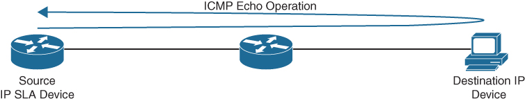
Figure 24-6 IP SLA Echo Operation
To configure any IP SLA operation, the ip sla operation-number command must be used to enter IP SLA configuration mode, where operation-number is the configuration for the individual IP SLA probe. This is necessary as there can be multiple IP SLA instances configured on a single device, all doing different operations or verification tasks. Once in IP SLA configuration mode, the command icmp-echo {destination-ip-address | destination-hostname} [source-ip {ip-address | hostname} | source-interface interface-name] is used to configure the destination IP address of the device or host to be monitored.
The next step is to specify how often the ICMP echo operation should run. This is accomplished by issuing the frequency seconds command. Note that many additional optional parameters are available for configuring IP SLA. This section only focuses on the basic setup and scheduling of IP SLA ICMP echo operations. Example 24-54 shows the process covered so far on R1.
Example 24-54 Configuring IP SLA ICMP Echo Operation on R1
R1(config)# ip sla 1
R1(config-ip-sla)# icmp-echo 192.168.14.100 source-interface Loopback0
R1(config-ip-sla-echo)# frequency 300
R1(config-ip-sla-echo)# end
R1(config)#
When the IP SLA configuration is complete, an important step is to schedule and activate the IP SLA operation that has been configured. This is where the ip sla schedule operation-number [life {forever | seconds}] [start-time {[hh:mm:ss] [month day | day month] | pending | now | after hh:mm:ss}] [ageout seconds] [recurring] command comes into play.
When the IP SLA operation is scheduled, it can be verified with the show ip sla configuration command. Example 24-55 illustrates the configuration steps to schedule the IP SLA 1 operation with a start time of now and a lifetime of forever. This example also shows the verification that it is running and configured properly.
Example 24-55 Scheduling IP SLA 1 on R1
R1(config)# ip sla schedule 1 life forever start-time now
R1(config)# do show ip sla configuration 1
IP SLAs Infrastructure Engine-III
Entry number: 1
Owner:
Tag:
Operation timeout (milliseconds): 5000
Type of operation to perform: icmp-echo
Target address/Source interface: 192.168.14.100/Loopback0
Type Of Service parameter: 0x0
Request size (ARR data portion): 28
Verify data: No
Vrf Name:
Schedule:
   Operation frequency (seconds): 300  (not considered if randomly scheduled)
   Next Scheduled Start Time: Start Time already passed
   Group Scheduled : FALSE
   Randomly Scheduled : FALSE
   Life (seconds): Forever
   Entry Ageout (seconds): never
   Recurring (Starting Everyday): FALSE
   Status of entry (SNMP RowStatus): Active
Threshold (milliseconds): 5000
Distribution Statistics:
   Number of statistic hours kept: 2
   Number of statistic distribution buckets kept: 1
   Statistic distribution interval (milliseconds): 20
Enhanced History:
History Statistics:
   Number of history Lives kept: 0
   Number of history Buckets kept: 15
   History Filter Type: None
Another very common use case for IP SLA is to monitor HTTP destinations for operation. This can be done by using the HTTP GET operation of IP SLA. In order to configure this type of monitor, as mentioned earlier, the ip sla operation-number command must be used to enter IP SLA configuration mode. When the operation number is specified, the next step is to configure the HTTP GET probe by issuing the command http {get | raw} url [name-server ip-address] [version version-number] [source-ip {ip-address | hostname}] [source-port port-number] [cache {enable | disable}] [proxy proxy-url].
When the probe is configured, as with any other IP SLA operation, this operation needs to be scheduled by using the command ip sla schedule operation-number [life {forever | seconds}] [start-time {[hh:mm:ss] [month day | day month] | pending | now | after hh:mm:ss}] [ageout seconds] [recurring]. Example 24-56 highlights these steps on R1.
Example 24-56 Configuring the IP SLA HTTP GET Operation on R1
R1(config)# ip sla 2
R1(config-ip-sla)# http get http://192.168.14.100
R1(config-ip-sla-http)# frequency 90
R1(config-ip-sla-http)# end
R1# configure terminal
Enter configuration commands, one per line.  End with CNTL/Z.
R1(config)# ip sla schedule 2 start-time now life forever
R1(config)# end
R1# show ip sla configuration 2
IP SLAs Infrastructure Engine-III
Entry number: 2
Type of operation to perform: http
Target address/Source address: 192.168.14.100/0.0.0.0
Target port/Source port: 80/0
Type Of Service parameters: 0x0
Vrf Name:
HTTP Operation: get
HTTP Server Version: 1.0
URL: http://192.168.14.100
Proxy:
Raw String(s):
Cache Control: enable
Owner:
Tag:
Operation timeout (milliseconds): 60000
Schedule:
   Operation frequency (seconds): 90  (not considered if randomly scheduled)
   Next Scheduled Start Time: Start Time already passed
   Group Scheduled : FALSE
   Randomly Scheduled : FALSE
   Life (seconds): Forever
   Entry Ageout (seconds): never
   Recurring (Starting Everyday): FALSE
   Status of entry (SNMP RowStatus): Active
Threshold (milliseconds): 5000
Distribution Statistics:
   Number of statistic hours kept: 2
   Number of statistic distribution buckets kept: 1
   Statistic distribution interval (milliseconds): 20
History Statistics:
   Number of history Lives kept: 0
   Number of history Buckets kept: 15
   History Filter Type: None


R1#
When IP SLA is set up and running appropriately, it can be monitored using the CISCO-RTTMON-MIB file with SNMP, and traps can be sent to an NMS via syslog. Documentation for this configuration can be found on the Cisco website.
Cisco DNA Center Assurance
Networks have grown very complex. The influx of mobile devices strains network resources and the network operations staff. Security has become one the most important pieces of the network, and users expect a better experience. Customers demand a simple way to manage Day 0–2 operations and require a scalable and simple approach to running the network. Cisco DNA Center Assurance provides a tool for handling the most relevant customer requirements. Traditionally, multiple management tools were required to meet the needs of the business in terms of managing, operating, and troubleshooting the network. This all changes with Cisco DNA Center Assurance. From a high level, Cisco DNA Center Assurance offers some of the following capabilities (as well as many more):
Cisco SD-Access fabric configuration
Software image management (SWIM)
Simplified provisioning for devices
Wireless network management
Simplified security policies
Configuration templates
Third-party integration
Network assurance
Plug and Play
This section covers some of the workflows that Cisco DNA Center Assurance is designed to help businesses with. Typically, when an issue arises in the network, a helpdesk ticket is created. However, by the time the network operations team gets the ticket assigned, the issue is either resolved on its own or the information provided in the ticket to assist with troubleshooting the issue is stale or out of date. Another typical scenario is that users say things like “last Tuesday at 3 p.m. I wasn’t able to get on the wireless network.” In a traditional network, if someone says she had an issue last week, there isn’t much that can be done about it. However, Cisco DNA Center Assurance has Network Time Travel, and it is as cool as it sounds. Network Time Travel acts as a digital video recorder (DVR) for the network. But rather than recording television and enabling the user to play back shows at a later time, Network Time Travel records what is going on in the environment using streaming telemetry and can play back something that happened in the past. It also can show how the network is performing now as well as use things such as sensors to provide predictive analytics on how the network will perform in the future. Figure 24-7 shows the main Cisco DNA Center page that is shown upon logging into the software.
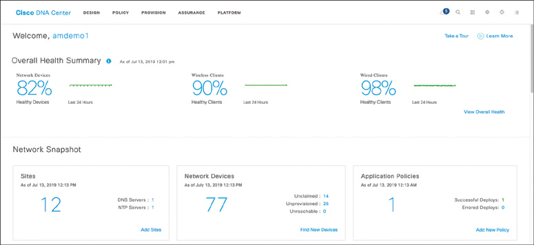
Figure 24-7 Cisco DNA Center Main Page
Cisco DNA Assurance is part of Cisco DNA Center. Assurance takes 30+ years of Cisco Technical Assistance Center (TAC) experience and puts it into a tool that uses machine learning to diagnose issues within a network. In addition to finding and diagnosing the issues, Assurance gives guided remediation steps to fix the issue. The Assurance tab is shown in Figure 24-8. Notice that it provides an overview of how the network is performing from an overall health perspective to a client perspective. It includes both wired and wireless clients. It also shows the top issues that are impacting the network. The health scores for each section enable you to see how the network is performing at quick glance.
If a user walks up and says she has an issue, the typical approach is to ask the user what her IP address or MAC address is so the network operations staff can jump from device to device, issuing multiple show commands to try to track down where the user is connected, as well as what issue might be causing the poor user experience. With Assurance, if a user walks up or a helpdesk ticket comes in, a simple search of the user’s name yields all the information necessary. Cisco DNA Center integrates with many other tools, such as Active Directory, Identity Services Engine (ISE), ServiceNow, and Infoblox. This is possible because of the open APIs and SDKs available for Cisco DNA Center. Because of the integration with Active Directory and ISE, all the context of the user is searchable in Cisco DNA Center.
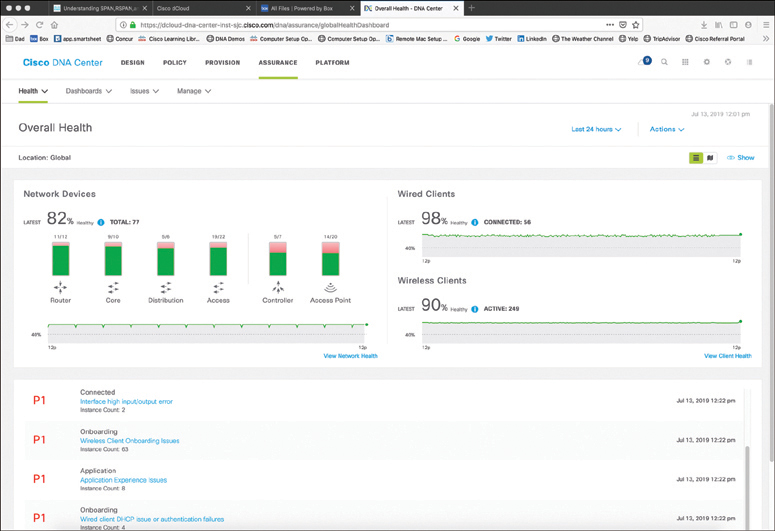
Figure 24-8 Cisco DNA Center Assurance Page
Say that a user named Grace has a problem. To search for Grace, you click the magnifying glass in the top-right corner and type her name in the search box. Because Cisco DNA Center is integrated with AD, all names populate as the search term is being typed. As you type Grace’s name, all users whose names start with G come up, then all users whose names start with Gr, and so on. Figure 24-9 shows the search box and Grace Smith as the matching user. It also shows all the devices on the network associated with Grace Smith—in this case, a PC, an iPad and an iPhone.
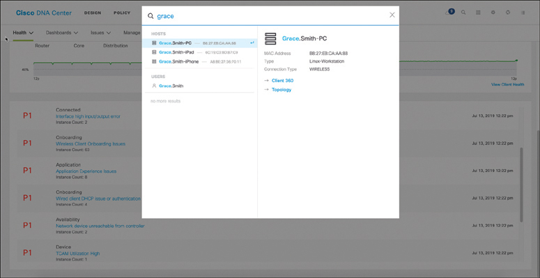
Figure 24-9 Cisco DNA Center Assurance Search Page
From this view, you can do many different things. You can click the user’s name to see details related to that specific user. You can click each device to see specifics about that device in the Client 360 view. Figure 24-10 shows the entire Client 360 view for the user Grace Smith. Notice that all three of Grace’s devices can be seen in this view, along with color-coded health scores for the devices.

Figure 24-10 Cisco DNA Center Assurance Client 360 Page
The amount of information that this screen provides is tremendous. Just for the selected iPad you can see that the following pieces of information have been gathered automatically:
Device type
OS version
MAC address
IPv4 address
VLAN ID
Connectivity status
When the device was last seen on the network
What device it is connected to
Wireless SSID
Last known location
Remember that all you have to do to get this information is search for Grace’s name.
The timeline in the Client 360 view shows issues that have impacted Grace. This is also a Network Time Travel capability. Since Assurance records the telemetry, it is possible to search back in time to see exactly what has affected Grace. The issues listed correlate to the timeline. The issue list changes based on the timeline and what time period is being investigated. Hovering over different times on the timeline allows you to see all the different issues that happened at various specific points in time. At first glance, it is easy to see some application latency issues are impacting Grace’s user experience.
Earlier in this chapter, you saw traceroute and ping used as troubleshooting tools when something is not working properly in the network environment. Assurance has a tool called Path Trace; the Run New Path Trace button is just underneath the issues listed on the Client 360 view. Path Trace is a visual traceroute and diagnostic tool that can be run periodically or continuously, with a specific refresh interval. Figure 24-11 shows a path trace being set up for Grace’s iPad to John’s PC, which are both wirelessly connected to the network. This path trace is set to refresh every 30 seconds.
The path trace output shows a topology view of the traceroute, and in this instance, Path Trace has also detected that there is an access control list (ACL) blocking the traffic from Grace’s iPad to John’s PC (see Figure 24-12).
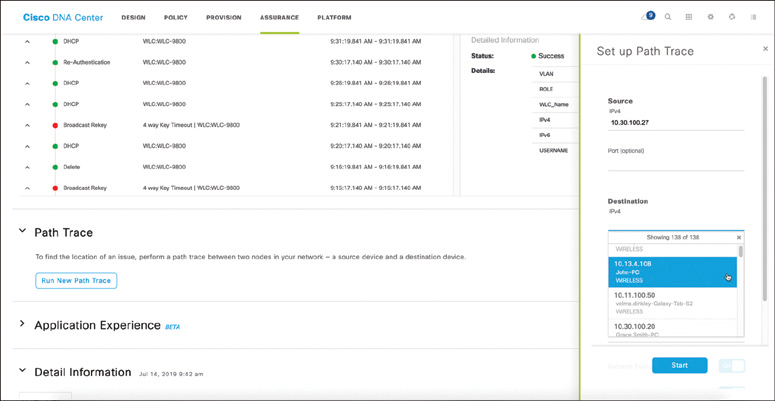
Figure 24-11 Cisco DNA Center Assurance Client 360 Path Trace
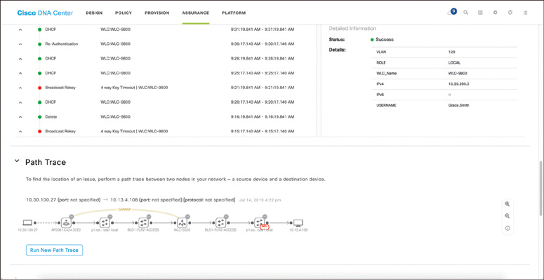
Figure 24-12 Cisco DNA Center Assurance Client 360 Path Trace Output
By hovering over the ACL entry, the following information can be seen:
The ACL’s name
The interface the ACL is applied to
The direction (ingress or egress)
The ACL result (permit or deny)
Figure 24-13 shows the access list information found in this example.

Figure 24-13 Cisco DNA Center Assurance Client 360 Path Trace ACL Information
By clicking on one of the issues listed under Grace’s Client 360 view, such as the P1 Onboarding issue, a user can investigate the root cause of the issue. Figure 24-14 shows the issues that are impacting Grace.
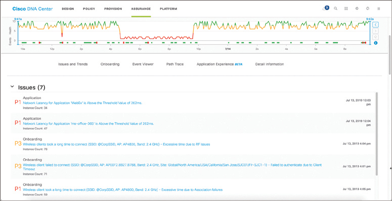
Figure 24-14 Cisco DNA Center Assurance Client 360 Issues
Figure 24-15 shows a large amount of useful information. The Impact of Last Occurrence states that this issue is impacting one building and seven wireless clients. There is also a detailed description of what is actually happening, along with suggested remediation steps to fix the issue. A user can click the arrows to see options such as average client onboarding times and impacted clients along with names, MAC address information, and the access points they are connected to. Although Cisco DNA Assurance can provide a wealth of information and details, this section shows only the high-level workflow used to diagnose and troubleshoot issues.
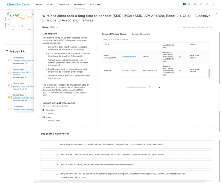
Figure 24-15 Cisco DNA Center Assurance Client 360 Root Cause and Guided Remediation Steps
Remember the traditional flow that network operations teams use to troubleshoot—logging in to multiple devices and trying to track down the root cause of an issue using traceroute, ping, and show? In less than the time it takes those teams to log in to a single device and issue all those commands, you can use Cisco DNA Center Assurance to quickly see the root cause of an issue and how to fix it. Thanks to open APIs and integration with helpdesk ticketing platforms such as ServiceNow, you can have all of the issues, impacted locations, path trace information, and remediation steps automatically added to helpdesk tickets so when the network operations staff gets a ticket, they already know what the issue is and how to fix it—without having to chase down the issue by using show commands on multiple devices in the network environment.
Exam Preparation Tasks
As mentioned in the section “How to Use This Book” in the Introduction, you have a couple of choices for exam preparation: the exercises here, Chapter 30, “Final Preparation,” and the exam simulation questions in the Pearson Test Prep Software Online.
Review All Key Topics
Review the most important topics in the chapter, noted with the key topics icon in the outer margin of the page. Table 24-11 lists these key topics and the page number on which each is found.
Table 24-11 Key Topics for Chapter 24
Key Topic Element |
Description |
Page |
Section |
Using tools such as ping and extended ping |
|
Section |
Using tools such as traceroute and extended traceroute |
|
Section |
Troubleshooting using debugging and conditional debugging |
|
OSPF Network Types and Hello/Dead Intervals |
||
Section |
Using SNMP for monitoring and troubleshooting |
|
Section |
Leveraging NetFlow information to analyze traffic statistics |
|
Section |
Understanding tools such as SPAN, RSPAN and ERSPAN for capturing network traffic |
|
Section |
Configuring tools such as SPAN, RSPAN, and ERSPAN to capture network traffic |
|
Section |
Leveraging on-box monitoring tools such as IP SLA to validate network and application performance |
|
Section |
Using DNA Center enhanced workflows to simplify design, provisioning, and troubleshooting of a network |
Complete Tables and Lists from Memory
There are no memory tables in this chapter.
Define Key Terms
Define the following key terms from this chapter, and check your answers in the glossary: