11. Nonisothermal Reactor Design: The Steady-State Energy Balance and Adiabatic PFR Applications

Search in book...
Toggle Font Controls
Create new playlist

Name your new playlist

Playlist description (optional)
Sign In

Email address

Password

Forgot Password?

or

Continue with Facebook

Continue with Google
Sign Up

Full Name

Email address

Confirm Email Address

Password

or

Continue with Facebook

Continue with Google

11. Nonisothermal Reactor Design: The Steady-State Energy Balance and Adiabatic PFR Applications

If you can’t stand the heat, get out of the kitchen.

—Harry S Truman

Overview. Because most reactions are not carried out isothermally, we now focus our attention on heat effects in chemical reactors. The basic CRE algorithm of mole balance, rate law, stoichiometry, combine, and evaluate used in Chapters 1–10 for isothermal reactor design is still valid for the design of nonisothermal reactors and we only need to add one more step, the energy balance to solve nonisothermal problems. The major difference lies in the method of evaluating the combined mole balances, rate law, and stoichiometry when temperature varies along the length of a PFR or when heat is removed from a CSTR.

This chapter is arranged as follows:

Section 11.1 shows why we need the energy balance and how it will be used to solve reactor design problems.
Section 11.2 develops the energy balance to a point where it can be applied to different types of reactors. It then gives the end result, relating temperature and conversion or reaction rate for the main types of reactors we have been studying.
Section 11.3 develops the user-friendly energy balances for reactors.
Section 11.4 discusses the adiabatic operation of reactors.
Section 11.5 shows how to determine the adiabatic equilibrium conversion and how to carry out interstage cooling.
Section 11.6 shows how to find the optimum inlet temperature to achieve the maximum conversion for adiabatic operation.
Section 11.7 closes the chapter with some thoughts on the type of critical thinking questions you could ask about the safety of your system.

11.1 Rationale

To identify the additional information necessary to design nonisothermal reactors, we consider the following example, in which a highly exothermic reaction is carried out adiabatically in a plug-flow reactor.

Example 11–1 What Additional Information Is Required?

The first-order liquid-phase reaction

A → B

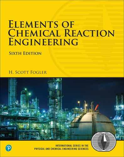
is carried out in a PFR. The reaction is exothermic and the reactor is operated adiabatically. As a result, the temperature will increase with conversion down the length of the reactor. Because T varies along the length of the reactor, k will also vary, which was not the case for isothermal plug-flow reactors.

Three line graphs map the variation of V in terms of components T, k, and X respectively. — The relationship between V with T, k, and X are graphically portrayed. The first graph compares V and T. The curve begins at T at a short distance above the origin, which increases gradually with increasing V. The second graph compares V and k. The curve begins at k at a short distance above the origin. Initially, the curve is flat and increases gradually with increasing V. The third graph compares V and X. The curve begins at the origin, which increases with increasing V.

Describe how to calculate the PFR reactor volume necessary for 70% conversion and plot the corresponding profiles for X and T.

Solution

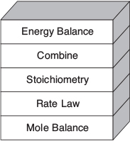
The same CRE algorithm can be applied to nonisothermal reactions as to isothermal reactions by adding one more step, the energy balance.

Mole Balance (design equation):

$\begin{matrix} \frac{d X}{d V} = \frac{- r_{A}}{F_{A 0}} & \begin{matrix} (E11-1.1) \end{matrix} \end{matrix}$
Rate Law:

$\begin{matrix} - r_{A} = {k C}_{A} & (E11-1.2) \end{matrix}$

Recalling the Arrhenius equation,

$\begin{matrix} k = k_{1} \exp [\frac{E}{R} (\frac{1}{T_{1}} - \frac{1}{T})] & \begin{matrix} (E11-1.3) \end{matrix} \end{matrix}$

we know that k is a function of temperature, T.
Stoichiometry (liquid phase): υ = υ₀

$\begin{matrix} C_{A} = C_{A0} (1 - X) & (E11-1.4) \end{matrix}$
Combining:

$\begin{matrix} - r_{A} = k_{1} \exp [\frac{E}{R} (\frac{1}{T_{1}} - \frac{1}{T})] C_{A 0} (1 - X) & \begin{matrix} (E11-1.5) \end{matrix} \end{matrix}$

Combining Equations (E11-1.1), (E11-1.2), and (E11-1.4), and canceling the entering concentration, C_A0, yields

$\begin{matrix} \frac{d X}{d V} = \frac{k (1 - X)}{v_{0}} & (E11-1.6) \end{matrix}$

Combining Equations (E11-1.3) and (E11-1.6) gives us

$\begin{matrix} \frac{d X}{d V} = k_{1} \exp [\frac{E}{R} (\frac{1}{T_{1}} - \frac{1}{T})] \frac{1 - X}{v_{0}} & \begin{matrix} (E11-1.7) \end{matrix} \end{matrix}$

Why we need the energy balance

Oops! We see that we need another relationship relating X and T or T and V to solve this equation. The energy balance will provide us with this relationship.

So we add another step to our algorithm; this step is the energy balance.
Energy Balance:

In this step, we will find the appropriate energy balance to relate temperature and conversion or reaction rate. For example, if the reaction is adiabatic, we will show that for equal heat capacities, $C_{P_{A}}$ and $C_{P_{B}}$ , and a constant heat of reaction, $Δ H_{Rx}^{\circ}$ , the temperature–conversion relationship for an adiabatic reaction (cf. Table 11-1) can be written in a form such as

$\begin{matrix} T = T_{0} + \frac{- Δ H_{R x}^{\circ}}{C_{P_{A}}} X & \begin{matrix} (E11-1.8) \end{matrix} \end{matrix}$

T₀

=

Entering CPB Temperature

${Δ H}_{Rx}^{o}$

=

Heat of Reaction

C_P_A

=

Heat Capacity of species A

We now have all the equations we need to solve for the conversion and temperature profiles. We simply type Equations (E11-1.7) and (E11-1.8) along with the parameters into Polymath, Wolfram, Python, or MATLAB; click the RUN button; and then carry out the calculation to a volume where 70% conversion is obtained.

Analysis: The purpose of this example was to demonstrate that for nonisothermal chemical reactions we need another step in our CRE algorithm, the energy balance. The energy balance allows us to solve for the reaction temperature, which is necessary in evaluating the specific reaction-rate constant k(T).

11.2 The Energy Balance

11.2.1 First Law of Thermodynamics

The goal of this section is to use the energy balance to develop user-friendly relationships with temperature that can be easily applied to chemical reactors. We begin with the application of the first law of thermodynamics, first to a closed system and then to an open system. A system is any bounded portion of the universe, moving or stationary, which is chosen for the application of the various thermodynamic equations. For a closed system, no mass crosses the system boundaries and the change in total energy of the system, dÊ, is equal to the heat flow to the system δQ, minus the work done by the system on the surroundings, δW. For a closed system, the energy balance is

$\begin{matrix} d \hat{E} = δ Q - δ W & \begin{matrix} (11-1) \end{matrix} \end{matrix}$

Closed system

The δs signify that δQ and δW are not exact differentials of a state function.

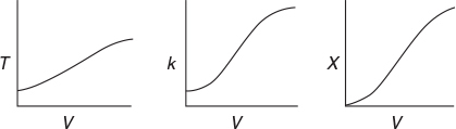
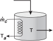
The continuous-flow reactors we have been discussing are open systems in which mass crosses the system boundary. We shall carry out an energy balance on the open system shown in Figure 11-1. For an open system in which some of the energy exchange is brought about by the flow of mass across the system boundaries, the energy balance for the case of only one species entering and leaving becomes

The energy balance between the incoming and outgoing energy in an open system is schematically explained. — **Figure 11-1** Energy balance on a well-mixed open system: schematic.

The flow of energy due to the incoming and outgoing molar flow rate, heat flow, and the energy dissipation due to work done is illustrated. The molar energy flow F subscript i (in) (Example: F subscript F0) enters the system along with the heat energy, H subscript i (in) (Example: H subscript A0). The system has the energy dissipation factor due to the work done on the surroundings W subscript s, along with the rate of heat flow from the surroundings Q. The molar and heat energies leave the system and it is mentioned as F subscript i (out) (Example F subscript A) and H subscript i out (Example H subscript A).

\begin{matrix} [\begin{matrix} \begin{matrix} \begin{matrix} \begin{matrix} \begin{matrix} \begin{matrix} \begin{matrix} \begin{matrix} \begin{matrix} Rate of \end{matrix} \\ accumulation \end{matrix} \end{matrix} \\ of energy \end{matrix} \end{matrix} \\ within the \end{matrix} \end{matrix} \\ system \end{matrix} \end{matrix}] & = & [\begin{matrix} \begin{matrix} \begin{matrix} \begin{matrix} \begin{matrix} \begin{matrix} \begin{matrix} \begin{matrix} \begin{matrix} Rate of flow \end{matrix} \\ of heat to \end{matrix} \end{matrix} \\ the system \end{matrix} \end{matrix} \\ from the \end{matrix} \end{matrix} \\ surroundings \end{matrix} \end{matrix}] & - & \begin{matrix} [\begin{matrix} \begin{matrix} \begin{matrix} \begin{matrix} \begin{matrix} \begin{matrix} \begin{matrix} \begin{matrix} \begin{matrix} \begin{matrix} Rate of work \end{matrix} \\ done by \end{matrix} \end{matrix} \\ the system \end{matrix} \end{matrix} \\ on the \end{matrix} \end{matrix} \end{matrix} \\ surroundings \end{matrix} \end{matrix}] \end{matrix} & + & [\begin{matrix} \begin{matrix} \begin{matrix} \begin{matrix} \begin{matrix} \begin{matrix} \begin{matrix} \begin{matrix} \begin{matrix} Rate of energy \end{matrix} \\ added to the \end{matrix} \end{matrix} \\ system by mass \end{matrix} \end{matrix} \\ flow into the \end{matrix} \end{matrix} \\ system \end{matrix} \end{matrix}] & - & [\begin{matrix} \begin{matrix} \begin{matrix} \begin{matrix} \begin{matrix} \begin{matrix} \begin{matrix} \begin{matrix} \begin{matrix} Rate of \end{matrix} \\ energy leaving \end{matrix} \end{matrix} \\ the system by mass \end{matrix} \end{matrix} \\ flow out of \end{matrix} \end{matrix} \\ the system \end{matrix} \end{matrix}] \\ \frac{d {\hat{E}}_{s y s}}{d t} & = & \dot{Q} & - & \dot{W} & + & F_{in} E_{in} & - & \begin{matrix} \begin{matrix} F_{out} E_{out} \end{matrix} & (11-2) \end{matrix} \\ (J/s) & = & (J/s) & - & (J/s) & + & (J/s) & - & (J/s) \end{matrix}

Energy balance on an open system

Typical units for each term in Equation (11-2) are (Joule/s). (Joule bio: http://www.corrosion-doctors.org/Biographies/JouleBio.htm.)

We will assume that the contents of the system volume are well mixed, an assumption that we could relax but that would require a couple of pages of text to develop, and the end result would be the same! The unsteady-state energy balance for an open well-mixed system that now has n species, each entering and leaving the system at their respective molar flow rate F_i (moles of i per time) and with their respective energy E_i (Joules per mole of i), is

\begin{matrix} \frac{d {\hat{E}}_{sys}}{d t} = \dot{Q} - \dot{W} + Σ_{i = l}^{n} E_{i} F_{i} |_{in} - Σ_{i = l}^{n} E_{i} F_{i} |_{out} \end{matrix} \begin{matrix} (11 - 3) \end{matrix}

The starting point

We will now discuss each of the terms in Equation (11-3).

11.2.2 Evaluating the Work Term

It is customary to separate the work term, $\dot{W}$ , into flow work and other work, ${\dot{W}}_{s}$ . The term ${\dot{W}}_{s}$ , often referred to as the shaft work, could be produced from such things as a stirrer in a CSTR or a turbine in a PFR. Flow work is work that is necessary to get the mass into and out of the system. For example, when shear stresses are absent, we write

\begin{matrix} \dot{W} = \overset{[Rate of flow work]}{\overset{⏞}{- {Σ_{i = 1}^{n} F_{i} P {\tilde{V}}_{i} |}_{in} + {Σ_{i = 1}^{n} F_{i} P {\tilde{V}}_{i} |}_{out}}} + {\dot{W}}_{s} & (11-4) \end{matrix}

Flow work and shaft work

where P is the pressure (Pa) [1 Pa = 1 Newton/m² = 1 kg·m/s²/m²] and is ${\tilde{V}}_{i}$ the specific molar volume of species i (m³/mol of i).

Let’s look at the units of the flow-work term, which is

$F_{i} \cdot P \cdot {\tilde{V}}_{i}$

where F_i is in mol/s, P is in Pa (1 Pa = 1 Newton/m²), and ${\tilde{V}}_{i}$ is in (m³/mol). Multiplying the units of each term in $(F_{i} P {\tilde{V}}_{i})$ through, we obtain the units of flow work, that is,

$\begin{matrix} F_{i} \cdot P \cdot {\tilde{V}}_{i} [=] \frac{mol}{s} \cdot \frac{Newton}{m^{2}} \cdot \frac{m^{2}}{mol} = (Newton \cdot m) \cdot \frac{1}{s} = Joules/s = Watts \end{matrix}$

We see that the units for flow work are consistent with the other terms in Equation (11-3), that is, (J/s) (http://www.corrosion-doctors.org/Biographies/WattBio.htm).

In most instances, the flow-work term is combined with those terms in the energy balance that represent the energy exchange by mass flow across the system boundaries. Substituting Equation (11-4) into (11-3) and grouping terms, we have

$\begin{matrix} \frac{d {\hat{E}}_{sys}}{d t} = \dot{Q} - {\dot{W}}_{s} + Σ_{i = 1}^{n} F_{i} (E_{i} + P {\tilde{V}}_{i}) |_{in} - Σ_{i = 1}^{n} F_{i} (E_{i} + P {\tilde{V}}_{i}) |_{out} & \begin{matrix} (11-5) \end{matrix} \end{matrix}$

Convention

Heat Added

$\dot{Q}$ = + –10 J/s

Heat Removed

$\dot{Q}$ = + –10 J/s

Work Done by System

${\dot{W}}_{s}$ = + –10 J/s

Work Done on System

${\dot{W}}_{s}$ = + –10 J/s

The energy E_i is the sum of the internal energy (U_i), the kinetic energy $(u_{i}^{2} / 2)$ , the potential energy (gz_i), and any other energies, such as electric or magnetic energy or light

$\begin{matrix} E_{i} = U_{i} + \frac{u_{i}^{2}}{2} + {g z}_{i} + other & \begin{matrix} (11-6) \end{matrix} \end{matrix}$

In almost all chemical reactor situations, the kinetic, potential, and “other” energy terms are negligible in comparison with the enthalpy, heat transfer, and work terms in the energy balance, and hence will be omitted, in which case

$\begin{matrix} E_{i} = U_{i} & \begin{matrix} (11-7) \end{matrix} \end{matrix}$

We recall that the enthalpy, H_i (J/mol), is defined in terms of the internal energy U_i (J/mol), and the product ${P \tilde{V}}_{i}$ (1 Pa · m³/mol = 1 J/mol):

$\begin{matrix} H_{i} = U_{i} + {P \tilde{V}}_{i} & \begin{matrix} (11-8) \end{matrix} \end{matrix}$

Enthalpy

Typical units of H_i are

$(H_{i}) = \frac{J}{mol i} or \frac{Btu}{lb-mol i} or \frac{cal}{mol i}$

Enthalpy carried into (or out of) the system can be expressed as the sum of the internal energy carried into (or out of) the system by mass flow plus the flow work:

$F_{i} H_{i} = F_{i} (U_{i} + {P \tilde{V}}_{i})$

Combining Equations (11-5), (11-7), and (11-8), we can now write the energy balance in the form

$\frac{{d \hat{E}}_{sys}}{d t} = \dot{Q} - {\dot{W}}_{s} + Σ_{i = 1}^{n} F_{i} H_{i} |_{in} - Σ_{i = 1}^{n} F_{i} H_{i} |_{out}$

The energy of the system at any instant in time, Ê_sys, is the sum of the products of the number of moles of each species in the system multiplied by their respective energies. The derivative of the E_sys term wrt time will be discussed in more detail when unsteady-state reactor operation is considered in Chapter 13.

We shall let the subscript “0” represent the inlet conditions. The conditions at the outlet of the chosen system volume will be represented by the unsubscripted variables.

\begin{matrix} \dot{Q} - {\dot{W}}_{s} + Σ_{i = l}^{n} F_{i o} H_{i o} - Σ_{i = l}^{n} F_{i} H_{i} = \frac{d {\hat{E}}_{sys}}{d t} \end{matrix} \begin{matrix} (11 - 9) \end{matrix}

A balancing scale illustrating the energy in and energy out is shown. — The energy balance is portrayed on a balancing scale. On one side elements such as F subscript i 0, H subscript i0, Q (over dot) represent the incoming energy. On the other side elements such as F subscript i, H subscript i, W (over dot) subscript s represent the energy going out.

In Section 11.1, we discussed that in order to solve reaction engineering problems with heat effects, we needed to relate temperature, conversion, and rate of reaction. The energy balance as given in Equation (11-9) is the most convenient starting point as we proceed to develop this relationship.

11.2.3 Overview of Energy Balances

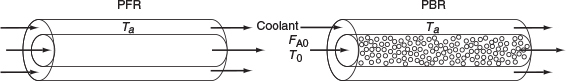
What is the plan? In the following pages, we manipulate Equation (11-9) in order to apply it to each of the reactor types we have been discussing: BR, PFR, PBR, and CSTR. The end result of the application of the energy balance to each type of reactor is shown in Table 11-1. These equations can be used in Step 5 of the algorithm discussed in Example 11-1. The equations in Table 11-1 relate temperature to conversion and to molar flow rates, and to the system parameters, such as the product of overall heat transfer coefficient, U, and heat exchange surface area, a, that is, Ua, with the corresponding ambient temperature, T_a, and the heat of reaction, ΔH_Rx.

Examples of How to Use Table 11-1. We now couple the energy balance equations in Table 11-1 with the appropriate reactor mole balance, rate law, and stoichiometry algorithm to solve reaction engineering problems with heat effects.

Table 11-1 gives the user-friendly reaction energy balances

End results of manipulating the energy balance (Sections 11.2.4, 12.1, and 12.3)

A graph representing the relationship between X and T portraying the linearity in the energy balance factor is shown. — TABLE 11-1 ENERGY BALANCES OF COMMON REACTORS

The heat exchange in a CSTR is portrayed by a small cylinder with an inductor whose two ends are denoted as m (over dot) subscript c and T subscript a. Also, an arrow indicates temperature T leaving out from the cylinder. — TABLE 11-1 ENERGY BALANCES OF COMMON REACTORS

For example, recall the rate law for a first-order reaction, Equation (E11-1.5) in Example 11-1

$\begin{matrix} - r_{A} = k_{1} exp [\frac{E}{R} (\frac{1}{T_{1}} - \frac{1}{T})] C_{A0} (1 - X) & \begin{matrix} (E11-1.5) \end{matrix} \end{matrix}$

which can be combined with the mole balance to find the concentration, conversion and temperature profiles (i.e., BR, PBR, PFR), exit concentrations, and conversion and temperature in a CSTR. We will now consider four cases of heat exchange in a PFR and PBR: (1) adiabatic, (2) co-current, (3) countercurrent, and (4) constant exchanger fluid temperature. We focus on adiabatic operation in this chapter and the other three cases in Chapter 12.

Case 1: Adiabatic. If the reaction is carried out adiabatically, then we use Equation (T11-1.B) for the reaction A → B in Example 11-1 to obtain

Adiabatic

$\begin{matrix} T = T_{0} + \frac{- Δ H_{Rx}^{\circ} X}{C_{P_{A}}} & (T11-1.B) \end{matrix}$

Consequently, we can now obtain –r_A as a function of X alone by first choosing X, then calculating T from Equation (T11-1.B), then calculating k from Equation (E11-1.3), and then finally calculating (–r_A) from Equation (E11-1.5)

The algorithm

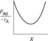
$\begin{matrix} Choose X \to calculate T \to calculate κ \to calculate - r_{A} \to calculate \frac{F_{A0}}{{- r}_{A}} \end{matrix}$

We can use this sequence to prepare a table of (F_A0/–r_A) as a function of X. We can then proceed to size PFRs and CSTRs. In the absolute worst case scenario, we could use the techniques in Chapter 2 (e.g., Levenspiel plots or the quadrature formulas in Appendix A). However, instead of using a Levenspiel plot, we will most definitely use software packages such as MATLAB, Wolfram, Python, or Polymath to solve our coupled differential energy and mole balance equations.

A levenspiel plot comparing X with F subscript A 0 over negative r subscript A is shown. The function F subscript A 0 decreases with increasing values of x, after which it rises dramatically.

Levenspiel plot

Cases 2, 3, and 4: Correspond to Co-Current Heat Exchange, Countercurrent Heat Exchange, and Constant Coolant Temperature T_C, respectively (Chapter 12). If there is cooling along the length of a PFR or PBR, we could then apply Equation (T11-1.D) to this reaction to arrive at two coupled differential equations.

In terms of conversion

$\begin{matrix} \frac{d X}{d V} = k_{1} exp [\frac{E}{R} (\frac{1}{T_{1}} - \frac{1}{T})] C_{A0} (1 - X) / F_{A0} \end{matrix}$

Non-adiabatic PFR

In terms of molar flow rate

$\frac{d F_{A}}{dV} = r_{A} = {- k C}_{A} = - k \frac{F_{A}}{υ} = - k_{1} \frac{F_{A}}{υ} \exp [\frac{E}{R} (\frac{1}{T_{1}} - \frac{1}{T})]$

either of which needs to be coupled with the energy balance

$\begin{matrix} \frac{d T}{d V} = \frac{r_{A} Δ H_{Rx} (T) - U a (T - T_{a})}{F_{A0} C_{P_{A}}} \end{matrix}$

which are easily solved using an ODE solver such as Polymath. If the temperature of the heat exchanger fluid (T_a) (e.g., coolant) is not constant, we add Equations (T11-1.K) or (T11-1.L) in Table 11-1 to the above equations and solve with Polymath, Wolfram, or MATLAB.

Heat Exchange in a CSTR. Similarly, for the case of the reaction A → B in Example 11-1 carried out in a CSTR, we could use Polymath, Python, Wolfram, or MATLAB to solve two nonlinear algebraic equations in X and T. These two equations are the combined mole balance

Non-adiabatic CSTR

$\begin{matrix} V = & \frac{F_{A0} X}{k_{1} \exp [\frac{E}{R} (\frac{1}{T_{1}} - \frac{1}{T})] C_{A0} (1 - X)} \end{matrix}$

and the application of Equation (T11-1.C), which is rearranged in the form

$T = \frac{F_{A0} X (- Δ H_{Rx}) + U A T_{a} + F_{A0} C_{P_{A}} T_{0}}{U A + C_{P_{A}} F_{A0}}$

From these three cases, (1) adiabatic PFR and CSTR, (2) PFR and PBR with heat effects, and (3) CSTR with heat effects, one can see how to couple the energy balances and mole balances. In principle, one could simply use Table 11-1 to apply to different reactors and reaction systems without further discussion. However, understanding the derivation of these equations will greatly facilitate the proper application to and evaluation of various reactors and reaction systems. Consequently, we now derive the equations given in Table 11-1.

Why bother? Here is why!!

Why bother to derive the equations in Table 11-1? Because I have found that students can apply these equations much more accurately to solve reaction engineering problems with heat effects if they have gone through the derivation to understand the assumptions and manipulations used in arriving at the equations in Table 11.1. That is, understanding these derivations, students are more likely to put the correct number in the correct equation symbol.

11.3 The User-Friendly Energy Balance Equations

We will now dissect the molar flow rates and enthalpy terms in Equation (11-9) to arrive at a set of equations we can readily apply to a number of reactor situations.

11.3.1 Dissecting the Steady-State Molar Flow Rates to Obtain the Heat of Reaction

To begin our journey, we start with the energy balance Equation (11-9), and then proceed to finally arrive at the equations given in Table 11-1 by first dissecting two terms:

The molar flow rates, F_i and F_i₀
The molar enthalpies, H_i, H_i₀[H_i ≡ H_i(T), and H_i₀ ≡ H_i(T₀)]

An illustration shows a computer, and represents the phrase "interactive computer games (ICG)."

An animated and “somewhat” humorous version of what follows for the derivation of the energy balance can be found in the reaction engineering games “Heat Effects 1” and “Heat Effects 2” on the CRE Web site, http://www.umich.edu/~elements/6e/icm/index.html. Here, equations talk to each other as they move around the screen, making substitutions and approximations to arrive at the equations shown in Table 11-1. Visual learners find these two ICGs a very useful resource (http://www.umich.edu/~elements/6e/icm/heatfx1.html).

We will now consider flow systems that are operated at steady state. The steady-state energy balance is obtained by setting (dÊ_sys/dt) equal to zero in Equation (11-9) in order to yield

Steady-state energy balance

$\begin{matrix} \dot{Q} - {\dot{W}}_{s} + Σ_{i = 1}^{n} F_{i 0} H_{i 0} - Σ_{i = 1}^{n} F_{i} H_{i} = 0 \end{matrix} \begin{matrix} (11 - 10) \end{matrix}$

To carry out the manipulations to write Equation (11-10) in terms of the heat of reaction, we shall use the generic reaction

$\begin{matrix} A + \frac{b}{a} B \to \frac{c}{a} C + \frac{d}{a} D & \begin{matrix} (2-2) \end{matrix} \end{matrix}$

The inlet and outlet summation terms in Equation (11-10) are expanded, respectively, to

In:

$\begin{matrix} Σ H_{i 0} F_{i 0} = H_{A 0} F_{A 0} + H_{B 0} F_{B 0} + H_{C 0} F_{C 0} + H_{D 0} F_{D 0} + H_{I 0} F_{I 0} & \begin{matrix} (11-11) \end{matrix} \end{matrix}$

and

Out:

$\begin{matrix} Σ H_{i} F_{i} = H_{A} F_{A} + H_{B} F_{B} + H_{C} F_{C} + H_{D} F_{D} + H_{I} F_{I} & (11-12) \end{matrix}$

where the capital subscript I represents inert species.

We next express the molar flow rates in terms of conversion. In general, the molar flow rate of species i for the case of no accumulation and a stoichio-metric coefficient ν_i is

F_i = F_A0 (Θ_i + ν_iX)

Specifically, for Reaction (2-2), $A + \frac{b}{a} B \to \frac{c}{a} C + \frac{d}{a} D$ , we have

F_A = F_A0 (1 — X)

$\begin{array}{l} \begin{matrix} F_{B} & = & F_{A0} [Θ_{B} - \frac{b}{a} X] \\ F_{C} & = & F_{A0} [Θ_{C} + \frac{c}{a} X] \\ F_{D} & = & F_{A0} [Θ_{D} + \frac{d}{a} X] \\ F_{1} & = & Θ_{1} F_{A0} \end{matrix}} & where Θ_{i} = \frac{F_{i 0}}{F_{A0}} \end{array}$

Steady-state operation

We can substitute these symbols for the molar flow rates into Equations (11-11) and (11-12), then subtract Equation (11-12) from (11-11) to give (11-13)

$\begin{matrix} Σ_{i = 1}^{n} F_{i 0} H_{i 0} - Σ_{i = 1}^{n} F_{i} H_{i} = & F_{A0} [(H_{A0} - H_{A}) + (H_{B0} - H_{B}) Θ_{B} \\ + (H_{C0} - H_{C}) Θ_{C} + (H_{D0} - H_{D}) Θ_{D} + (H_{I0} - H_{I}) Θ_{I}] \\ \begin{matrix} \begin{matrix} \begin{matrix} \begin{matrix} \begin{matrix} - (\frac{d}{a} H_{D} + \frac{c}{a} H_{C} - \frac{b}{a} H_{B} - H_{A}) F_{A0} X \end{matrix} \\ ⏟ \end{matrix} \end{matrix} \end{matrix} \\ Δ H_{Rx} \end{matrix} & (11-13) \end{matrix}$

The term in parentheses that is multiplied by F_A0X is called the heat of reaction at temperature T and is designated ΔH_Rx(T).

$\begin{matrix} Δ H_{Rx} (T) = \frac{d}{a} H_{D} (T) + \frac{c}{a} H_{C} (T) - \frac{b}{a} H_{B} (T) - H_{A} (T) \end{matrix} \begin{matrix} (11 - 14) \end{matrix}$

Heat of reaction at temperature T

All enthalpies (e.g., H_A, H_B) are evaluated at a temperature T in the reactor and, consequently, [ΔH_Rx(T)] is the heat of reaction at that specific temperature T. The heat of reaction is always given per mole of the species that is the basis of calculation, that is, species A (Joules per mole of A reacted).

Substituting Equation (11-14) into (11-13) and reverting to summation notation for the species, Equation (11-13) becomes

$\begin{matrix} Σ_{i = 1}^{n} F_{i 0} H_{i 0} - Σ_{i = 1}^{n} F_{i} H_{i} = F_{A 0} Σ_{i = 1}^{n} Θ_{i} (H_{i 0} - H_{i}) - Δ H_{R x} (T) F_{A 0} X & \begin{matrix} (11-15) \end{matrix} \end{matrix}$

Combining Equations (11-10) and (11-15), we can now write the steady-state, that is, (dÊ_sys/dt = 0), energy balance in a more usable form:

One can use this form of the steady-state energy balance if the enthalpies are available.

$\begin{matrix} \dot{Q} - {\dot{W}}_{s} + F_{A0} Σ_{i = 1}^{n} Θ_{i} (H_{i 0} - H_{i}) - Δ H_{Rx} (T) F_{A0} X = 0 \end{matrix} \begin{matrix} (11 - 16) \end{matrix}$

If a phase change takes place during the course of a reaction, this is the form of the energy balance (i.e., Equation (11-16)) that must be used.

A scalpel with drops of liquid dripping from the blade.

11.3.2 Dissecting the Enthalpies

We are neglecting any enthalpy changes resulting from mixing so that the partial molal enthalpies are equal to the molal enthalpies of the pure components. The molal enthalpy of species i at a particular temperature and pressure, H_i, is usually expressed in terms of an enthalpy of formation of species i at some reference temperature T_R, $H_{i}^{o} (T_{R})$ , plus the change in enthalpy, ΔH_Qi, that results when the temperature is raised from the reference temperature, T_R, to some temperature T

$\begin{matrix} H_{i} = H_{i}^{\circ} (T_{R}) + Δ H_{Q i} & \begin{matrix} (11-17) \end{matrix} \end{matrix}$

The reference temperature at which is H_i^°(T_R) given is usually 25°C. For any substance i that is being heated from T₁ to T₂ in the absence of phase change

$\begin{matrix} Δ H_{Q i} = \int_{T_{1}}^{T_{2}} C_{P_{i}} d T & \begin{matrix} (11-18) \end{matrix} \end{matrix}$

No phase change

Typical units of the heat capacity, C_{P_i}, are

$(C_{P_{i}}) = \frac{J}{(mol of i) (K)} o r \frac{Btu}{(l b mol of i) ({}^{\circ}R)} o r \frac{cal}{(mol of i) (K)}$

A large number of chemical reactions carried out in industry do not involve phase change. Consequently, we shall further refine our energy balance to apply to single-phase chemical reactions. Under these conditions, the enthalpy of species i at temperature T is related to the enthalpy of formation at the reference temperature T_R by

$\begin{matrix} H_{i} (T) = H_{i}^{\circ} (T_{R}) + \int_{T_{R}}^{T} C_{P_{i}} d T & \begin{matrix} (11-19) \end{matrix} \end{matrix}$

If phase changes do take place in going from the temperature for which the enthalpy of formation is given and the reaction temperature T, Equation (11-17) must be used instead of Equation (11-19).

The heat capacity at temperature T is frequently expressed as a quadratic function of temperature; that is

$\begin{matrix} C_{P_{i}} = α_{i} + β_{i} T + γ_{i} T^{2} & \begin{matrix} (11-20) \end{matrix} \end{matrix}$

However, while this text will consider only constant heat capacities, the PRS R11.1 on the CRE Web site has examples with variable heat capacities (http://www.umich.edu/~elements/6e/11chap/prof.html).

An icon of the reference shelf with books.

To calculate the change in enthalpy (H_i — H_i₀) when the reacting fluid is heated without phase change from its entrance temperature, T_i₀, to a temperature T, we integrate Equation (11-19) for constant C_P_i to write

$\begin{matrix} \begin{matrix} H_{i} - H_{i 0} & = [H_{i}^{\circ} (T_{R}) + \int_{T_{R}}^{T} C_{P_{i}} d T] - [H_{i}^{\circ} (T_{R}) + \int_{T_{R}}^{T_{i 0}} C_{P_{i}} d T] \\ = \int_{T_{R}}^{T} C_{P_{i}} d T = C_{P_{i}} [T - T_{i 0}] \end{matrix} & \begin{matrix} (11-21) \end{matrix} \end{matrix}$

Substituting for H_i and H_i₀ into Equation (11-16) yields

$\begin{matrix} \dot{Q} - {\dot{W}}_{s} + F_{A0} Σ_{i = 1}^{n} Θ_{i} C_{P_{i}} (T - T_{i 0}) - Δ H_{Rx} (T) F_{A0} X = 0 \end{matrix} \begin{matrix} (11 - 22) \end{matrix}$

Result of dissecting the enthalpies

11.3.3 Relating ΔH_Rx(T), ${Δ H}_{Rx}^{o} (T_{R})$ , and ΔC_P

Recall that the heat of reaction at temperature T was given in terms of the enthalpy of each reacting species at temperature T in Equation (11-14); that is

$\begin{matrix} Δ H_{R x} (T) = \frac{d}{a} H_{D} (T) + \frac{c}{a} H_{C} (T) - \frac{b}{a} H_{B} (T) - H_{A} (T) & \begin{matrix} (11-14) \end{matrix} \end{matrix}$

where the enthalpy of each species is given by

$\begin{matrix} H_{i} (T) = H_{i}^{\circ} (T_{R}) + \int_{T_{R}}^{T} C_{P_{c}} d T = H_{i}^{\circ} (T_{R}) + C_{P_{i}} (T - T_{R}) & \begin{matrix} (11-19) \end{matrix} \end{matrix}$

If we now substitute for the enthalpy of each species, we have

$\begin{matrix} Δ H_{Rx} (T) & = [\frac{d}{a} H_{D}^{\circ} (T_{R}) + \frac{c}{a} H_{C}^{\circ} (T_{R}) - \frac{b}{a} H_{B}^{\circ} (T_{R}) - H_{A}^{\circ} (T_{R})] \\ + [\frac{d}{a} C_{P_{D}} + \frac{c}{a} C_{P_{c}} - \frac{b}{a} C_{P_{B}} - C_{P_{A}}] (T - T_{R}) \end{matrix} (11 - 23)$

For the generic reaction $A + \frac{b}{a} B \to \frac{c}{a} C + \frac{d}{a} D$

The first term in brackets on the right-hand side of Equation (11-23) is the heat of reaction at the reference temperature T_R

$\begin{matrix} Δ H_{Rx}^{\circ} (T_{R}) = \frac{d}{a} H_{D}^{\circ} (T_{R}) + \frac{c}{a} H_{C}^{\circ} (T_{R}) - \frac{b}{a} H_{B}^{\circ} (T_{R}) - H_{A}^{\circ} (T_{R}) \end{matrix} \begin{matrix} (11 - 24) \end{matrix}$

The enthalpies of formation of many compounds, $H_{i}^{o} (T_{R})$ , are usually tabulated at 25°C and can readily be found in the Handbook of Chemistry and Physics and similar handbooks.¹ That is, we can look up the heats of formation at T_R, then calculate the heat of reaction at this reference temperature. The heat of combustion (also available in these handbooks) can be used to determine the enthalpy of formation, $H_{i}^{o} (T_{R})$ , and this method of calculation is also described in these handbooks. From these values of the standard heat of formation, $H_{i}^{o} (T_{R})$ , we can calculate the heat of reaction at the reference temperature T_R using Equation (11-24).

¹ CRC Handbook of Chemistry and Physics, 95th ed. Boca Raton, FL: CRC Press, 2014.

The second term in brackets on the right-hand side of Equation (11-23) is the overall change in the heat capacity per mole of A reacted, ΔC_P,

ΔC_P

$\begin{matrix} Δ C_{P} = \frac{d}{a} C_{P_{D}} + \frac{c}{a} C_{P_{C}} - \frac{b}{a} C_{P_{B}} - C_{P_{A}} \end{matrix} \begin{matrix} (11-25) \end{matrix}$

Combining Equations (11-25), (11-24), and (11-23) gives us

$\begin{matrix} Δ H_{Rx} (T) = Δ H_{Rx}^{\circ} (T_{R}) + Δ C_{P} (T - T_{R}) \end{matrix} \begin{matrix} (11-26) \end{matrix}$

Heat of reaction at temperature T ΔH_Rx(T)

Equation (11-26) gives the heat of reaction at any temperature T in terms of the heat of reaction at a reference temperature (usually 298 K) and the ΔC_P term. Techniques for determining the heat of reaction at pressures above atmospheric can be found in Chen.² We note that for the reaction of hydrogen and nitrogen at 400°C, it was shown that the heat of reaction increased by only 6% as the pressure was raised from 1 to 200 atm! Consequently, we will neglect the effects of pressure on the heat of reaction.

² N. H. Chen, Process Reactor Design, Needham Heights, MA: Allyn and Bacon, 1983, p. 26.

Example 11–2 Heat of Reaction

Calculate the heat of reaction for the synthesis of ammonia from hydrogen and nitrogen at 150°C in terms of (kcal/mol) of N₂ reacted and also in terms of (kJ/mol) of H₂ reacted.

Solution

N₂ + 3H₂ → 2NH₃

To calculate the heat of reaction at the reference temperature T_R, we will use the heats of formation of the reacting species obtained from Perry’s Chemical Engineers’ Handbook or the Handbook of Chemistry and Physics.³

³ D. W. Green and R. H. Perry, eds., Perry’s Chemical Engineers’ Handbook, 8th ed. New York: McGraw-Hill, 2008.

The enthalpies of formation at 25°C are

$H_{N H_{3}}^{o} (T_{R}) = - 11020 \frac{c a 1}{m o l N H_{3}}, H_{H_{2}} = 0, and H_{N_{2}} = 0$

Note: The heats of formation of all elements (e.g., H₂, N₂) are by definition zero at 25°C.

We now can calculate $Δ H_{Rx}^{o} (T_{R})$ , using Equation (11-24) and inserting the heats of formation of the products (e.g., NH₃) multiplied by their appropriate stoichiometric coefficients (2 for NH₃) minus the heats of formation of the reactants (e.g., N₂, H₂) multiplied by their stoichiometric coefficient (e.g., 3 for H₂, 1 of N₂)

$\begin{matrix} Δ H_{R x}^{\circ} (T_{R}) & = & 2 H_{N H_{3}}^{\circ} (T_{R}) - 3 H_{H_{2}}^{\circ} (T_{R}) - H_{N_{2}}^{\circ} (T_{R}) (E11-2.1) \end{matrix}$

$\begin{matrix} Δ H_{Rx}^{\circ} (T_{R}) & = & {2H}_{{NH}_{3}}^{\circ} (T_{R}) - 3 (0) - 0 = 2 H_{{NH}_{3}}^{\circ} \\ = & 2 (- 11020) \frac{cal}{{mol N}_{2}} \\ = & - 22040 cal/mol N_{2} reacted \\ Δ H_{Rx}^{\circ} (298 K) & = & - 22.04 kcal/mol N_{2} reacted \end{matrix}$

or in terms of kJ/mol (recall: 1 kcal = 4.184 kJ)

$\begin{matrix} Δ H_{Rx}^{\circ} (298 K) & = & - 9 2. 22 kJ/mol N_{2} reacted \end{matrix}$

Exothermic reaction

The minus sign indicates that the reaction is exothermic.

If the heat capacities are constant or if the mean heat capacities over the range 25°C–150°C are readily available, the determination of ΔH_Rx at 150°C is quite simple. (E11-2.2)

$\begin{matrix} \begin{matrix} C_{P_{H_{2}}} & = & 6.992 cal/mol H_{2} \cdot K \\ C_{P_{N_{2}}} & = & 6.984 cal/mol N_{2} \cdot K \\ C_{P_{{NH}_{3}}} & = & 8.92 cal/mol {NH}_{3} \cdot K \\ Δ C_{p} & = & 2 C_{P_{{NH}_{3}}} - 3 C_{P_{H_{2}}} - C_{P_{N_{2}}} \\ = & 2 (8.92) - 3 (6.992) - 6.984 \\ = & - 10.12 {cal/mol N}_{2} reacted \cdot K \end{matrix} & \begin{matrix} (E11-2.2) \end{matrix} \end{matrix}$

$\begin{matrix} Δ H_{Rx} (T) & = & Δ H_{Rx}^{\circ} (T_{R}) + Δ C_{P} (T - T_{R}) \\ Δ H_{Rx} (423 K) & = & - 22040 + (- 10.12) (423-298) \begin{matrix} (11-26) \end{matrix} \\ = & - 23310 {cal/mol N}_{2} = - 23.31 {cal/mol N}_{2} \end{matrix}$

in terms of kJ/mol

$\begin{matrix} \begin{matrix} \begin{matrix} Δ H_{Rx}^{\circ} (298 K) & = & - 23.3 kcal/mol N_{2} \times 4.184 kJ/kcal \end{matrix} \end{matrix} \end{matrix}$

$\begin{matrix} \begin{matrix} Δ H_{Rx} (423 K) & = & - 97.5 {kJ/mol N}_{2} \end{matrix} & Answer \end{matrix}$

The heat of reaction based on the moles of H₂ reacted is

$\begin{matrix} Δ H_{Rx} (423 K) = \frac{1 {mol N}_{2}}{3 {mol H}_{2}} (- 97.53 \frac{kJ}{{mol N}_{2}}) \\ Δ H_{Rx} (423 K) = - 32.51 \frac{kJ}{{mol H}_{2}} at 423 K Answer \end{matrix}$

Analysis: This example showed (1) how to calculate the heat of reaction with respect to a given species, given the heats of formation of the reactants and the products, and (2) how to find the heat of reaction with respect to one species, given the heat of reaction with respect to another species in the reaction. Finally, (3) we also saw how the heat of reaction changed as we changed the temperature.

Now that we see that we can calculate the heat of reaction at any temperature, let’s substitute Equation (11-22) in terms of ΔH_R(T_R) and ΔC_P, that is, Equation (11-26). The steady-state energy balance is now

$\begin{matrix} \dot{Q} - {\dot{W}}_{s} - F_{A0} Σ_{i = 1}^{n} Θ_{i} C_{P_{i}} (T - T_{i 0}) - [Δ H_{Rx}^{\circ} (T_{R}) + Δ C_{P} (T - T_{R})] F_{A0} X = 0 \end{matrix} \begin{matrix} (11-27) \end{matrix}$

Energy balance in terms of mean or constant heat capacities

From here on, for the sake of brevity we will let

$Σ = Σ_{i = 1}^{n}$

unless otherwise specified.

In most systems, the work term, ${\dot{W}}_{s}$ , can be neglected (note the exception in the California Professional Engineers’ Registration Exam Problem P12-6_B at the end of Chapter 12). Neglecting ${\dot{W}}_{s}$ , the energy balance becomes

$\begin{matrix} \dot{Q} - F_{A0} Σ Θ_{i} C_{P_{i}} (T - T_{i 0}) - [Δ H_{Rx}^{\circ} (T_{R}) + Δ C_{P} (T - T_{R})] F_{A0} X = 0 \end{matrix} \begin{matrix} (11-28) \end{matrix}$

We set T_i0 = T₀

In almost all of the systems we will study, the reactants will be entering the system at the same temperature; therefore, we will set T_i₀ = T₀.

We can use Equation (11-28) to relate temperature and conversion and then proceed to evaluate the algorithm described in Example 11-1. However, unless the reaction is carried out adiabatically, Equation (11-28) is still difficult to evaluate because in non-adiabatic reactors, the heat added to or removed from the system can vary along the length of the reactor or $\dot{Q}$ can vary with time. This problem does not occur in reactors operated adiabatically, a situation often found in industry, therefore, the adiabatic tubular reactor will be analyzed first.

11.4 Adiabatic Operation ∴ $\dot{Q}$ = 0

Reactions in industry are frequently carried out adiabatically with heating or cooling provided either upstream or downstream. Consequently, analyzing and sizing adiabatic reactors is an important task.

11.4.1 Adiabatic Energy Balance

In the previous section, we derived Equation (11-28), which relates conversion to temperature and the heat added to the reactor, $\dot{Q}$ . Let’s stop a minute (actually it will probably be more like a couple of days) and consider a system with the special set of conditions of no work, ${\dot{W}}_{s} = 0$ , adiabatic operation $\dot{Q} = 0$ , letting T_i0 = T₀ and then rearranging Equation 11-28 into the form to express the conversion X as a function of temperature, that is,

For adiabatic operation, Example 11.1 can now be solved!

$\begin{matrix} X = \frac{Σ Θ_{i} C_{P_{i}} (T - T_{0})}{- [Δ H_{Rx}^{\circ} (T_{R}) + Δ C_{P} (T - T_{R})]} \end{matrix} (11-29)$

In many instances, the ΔC_P(T — T_R) term in the denominator of Equation (11-29) is negligible with respect to the ${Δ H}_{Rx}^{o}$ term, so that a plot of X versus T will usually be linear, as shown in Figure 11-2. To remind us that the conversion in this plot was obtained from the energy balance rather than the mole balance, it is given the subscript EB (i.e., X_EB) in Figure 11-2.

Relationship between X and T for adiabatic exothermic reactions

A graph representing the relationship between X and T for an adiabatic exothermic reaction is shown. — **Figure 11-2** Adiabatic temperature–conversion relationship.

A plot representing a linear conversion is shown. The horizontal axis represents T and the vertical axis represents X subscript EB. The plots show an increasing line from the origin at T subscript 0. It is observed that X subscript EB increases with T linearly, for Q (over dot) and W (over dot) equals 0. The line indicates CSTR, PFR, PBR, and Batch.

Equation (11-29) applies to a CSTR, PFR, or PBR, and also to a BR (as will be shown in Chapter 13). For Q̇ = 0 and Ẇ_s = 0, Equation (11-29) gives us the explicit relationship between X and T needed to be used in conjunction with the mole balance to solve a large variety of chemical reaction engineering problems as discussed in Section 11.1.

We can rearrange Equation (11-29) to solve for temperature as a function of conversion; that is

$\begin{matrix} T = \frac{X [- Δ H_{Rx}^{\circ} (T_{R})] + Σ Θ_{i} {C_{P_{i}}}_{} T_{0} + X Δ C_{P} T_{R}}{Σ Θ_{i} C_{P_{i}} + X Δ C_{P}} \end{matrix} (11-30)$

Energy balance for adiabatic operation of PFR

11.4.2 Adiabatic Tubular Reactor

Either Equation (11-29) or Equation (11-30) will be coupled with the differential mole balance

$F_{A 0} \frac{d X}{d V} = - r_{A} (X, T)$

to obtain the temperature, conversion, and concentration profiles along the length of the reactor. The algorithm for solving PBRs and PFRs operated adiabatically will be illustrated by using a first-order reversible elementary reaction A ⇄ B as an example. Table 11-2 shows the algorithm using conversion, X, as the dependent variable while Table 11-3 shows the algorithm for solving the same reaction using molar flow rates instead of conversion.

The solution to reaction engineering problems today is to use software packages with ordinary differential equation (ODE) solvers, such as Polymath, MATLAB, Python, or Wolfram, to solve the coupled mole balance and energy balance differential equations.

We will now apply the algorithm in Table 11-2 and the solution procedure in Table 11-3 to a real reaction.

An illustration depicts footsteps, and represents the phrase "following the algorithm".

TABLE 11-2 ADIABATIC PFR/PBR ALGORITHM

The elementary reversible gas-phase reaction

A ⇄ B

is carried out in a PFR in which pressure drop is neglected and species A and inert I enter the reactor.

Mole Balance:

$\begin{matrix} \frac{d X}{d V} = \frac{{- r}_{A}}{F_{A0}} & (T11-21) \end{matrix}$
Rate Law:

$\begin{matrix} - r_{A} = k (C_{A} - \frac{C_{B}}{K_{e}}) & (T11-2.2) \end{matrix}$

$\begin{matrix} k = k_{1} (T_{1}) \exp [\frac{E}{R} (\frac{1}{T_{1}} - \frac{1}{T})] & (T11-2.3) \end{matrix}$

and for the case ΔC_P = 0

$\begin{matrix} K_{e} = K_{e 2} (T_{2}) \exp [\frac{Δ H_{Rx}^{\circ}}{R} (\frac{1}{T_{2}} - \frac{1}{T})] & (T11-2.4) \end{matrix}$
Stoichiometry: Gas, ɛ = 0, P = P₀ ∴ P ≡ 1

$\begin{matrix} C_{A} = C_{A0} (1 - X) \frac{T_{o}}{T} & (T11-2.5) \end{matrix}$

$\begin{matrix} C_{B} = C_{A0} X \frac{T_{o}}{T} & (T11.26) \end{matrix}$
Combine:

$\begin{matrix} - r_{A} = k C_{A0} [(1 - X) - \frac{X}{K_{e}}] \frac{T_{0}}{T} & (T11-2.7) \end{matrix}$

At equilibrium –r_A ≡ 0, and we can solve Equation (T11-2.7) for the equilibrium conversion, X_e

$\begin{matrix} X_{e} = \frac{K_{e}}{1 + K_{e}} & (T11-2.8) \end{matrix}$
Energy Balance:

To relate temperature and conversion, we apply the energy balance to an adiabatic PFR. If all species enter at the same temperature, T_i0 = T₀.

Solving Equation (11-30) for the case of ΔC_P = 0 and when only Species A and an inert I enter, we find the temperature as a function of conversion to be

$\begin{matrix} T = T_{0} + \frac{X [- Δ {H^{\circ}}_{Rx} (T_{R})]}{C_{P_{A}} + Θ_{I} C_{P_{I}}} & (T11-2.9) \end{matrix}$

Using either Equation (11-29) or Equation (T11-2.9), we find the conversion predicted as a function of temperature from the energy balance is

$\begin{matrix} X_{EB} = \frac{(C_{P_{A}} + Θ_{I} C_{P_{I}}) (T - T_{0})}{- Δ {H^{\circ}}_{Rx} (T_{R})} & (T11-2.10) \end{matrix}$

We have added the subscript to the conversion to denote that it was calculated from the energy balance, rather than from the mole balance. Equations (T11-2.1)–(T11-2.10) can easily be solved using either Simpson’s rule or an ODE solver.

Parameter values for this example (e.g., $Δ H_{Rx}^{\circ}$ , k₁) are given in Steps 5 and 6 in Table 11-3.

TABLE 11-3 SOLUTION PROCEDURES FOR ELEMENTARY ADIABATIC GAS-PHASE PFR/PBR REACTOR

Moles as the Dependent Variable

Mole Balances

$\begin{matrix} \frac{d F_{A}}{d W} = & r_{A}^{'} \\ \frac{d F_{B}}{d W} = & r_{B}^{'} \end{matrix}$
Rates

$\begin{array}{c} Rate Law: - r_{A}^{'} = & k (C_{A} - \frac{C_{B}}{K_{C}}) \\ {Relative Rates: r}_{B}^{'} = & - r_{A}^{'} \\ k = k_{1} (T_{1}) \exp & [\frac{E}{R} (\frac{1}{T_{1}} - \frac{1}{T})] \\ K_{C} = K_{C2} (T_{2}) \exp & [\frac{Δ {H^{\circ}}_{Rx}}{R} (\frac{1}{T_{2}} - \frac{1}{T})] \end{array}$

Recall that for δ ≡0, K_C ≡ K_e.
Stoichiometry

$\begin{array}{l} C_{A} & = & C_{T0} \frac{F_{A}}{F_{T}} \frac{T_{0}}{T} p \\ C_{B} & = & C_{T0} \frac{F_{B}}{F_{T}} \frac{T_{0}}{T} p \\ F_{T} & = & F_{A} + F_{B} + F_{I} \\ \frac{d p}{d W} & = & - \frac{α}{2 p} \frac{T}{T_{0}} \frac{F_{T}}{F_{T0}} \\ X & = & \frac{F_{A0} - F_{A}}{F_{A0}} \end{array}$
Energy

$T = T_{0} + \frac{- Δ {H^{\circ}}_{Rx} X}{C_{P_{A}} + Θ_{I} C_{P_{I}}}$
Parameter Evaluation

$\begin{array}{l} T_{1} = 298 K & Θ_{I} = 1 & C_{T0} = 1.0 {mol/dm}^{3} \\ T_{2} = 298 K & K_{C2} = 75000 & Δ {H^{\circ}}_{Rx} = - 14000 cal/mol \\ C_{P_{A}} = 25 cal/mol/K & k_{1} = {3.5 X 10}^{- 5} {min}^{- 1} & E = 10000 cal/mol \\ C_{P_{I}} = 50 cal/mol/K & F_{A0} = 5 mol/min \end{array}$
Entering Conditions

When V = 0, F_A0 = 5, F_B = 0, and T₀ = 480 K

These values are also used in LEP 11-6 on the Web site.

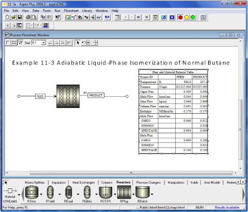
Example 11–3 Adiabatic Liquid-Phase Isomerization of Normal Butane

Normal butane, C₄H₁₀, is to be isomerized to isobutane in a plug-flow reactor. Iso-butane is a valuable product that is used in the manufacture of gasoline additives. For example, isobutane can be further reacted to form iso-octane. The 2014 selling price of n-butane was $1.5/gal, while the trading price of isobutane was $1.75/gal.^†

^†Once again, you can buy a cheaper generic brand of n–C₄H₁₀ at the Sunday markets in downtown Riça, Jofostan, where there will be a special appearance and lecture by Jofostan’s own Prof. Dr. Sven Köttlov on February 29th, at the CRE booth.

This elementary reversible reaction is to be carried out adiabatically in the liquid phase under high pressure using essentially trace amounts of a liquid catalyst that gives a specific reaction rate of 31.1 h^–1 at 360 K. We want to process 100000 gal/day (163 kmol/h) and achieve 70% conversion of n-butane from a mixture 90 mol % n-butane and 10 mol % i-pentane, which is considered an inert. The feed enters at 330 K.

Set up the CRE algorithm to calculate the PFR volume necessary to achieve 70% conversion.
Use an ODE software package (e.g., Polymath) to solve the CRE algorithm to plot and analyze X, X_e, T, and –r_A down the length (volume) of a PFR to achieve 70% conversion.
Calculate the CSTR volume for 40% conversion.

The economic incentive $ = 1.75/gal versus 1.50/gal

Additional information:

$\begin{matrix} Δ H_{Rx}^{\circ} = - 6900 J/mol n -butane, Activation energy = 65.7 kJ/mol \\ K_{C} = 3.03 at 60^{\circ} C, C_{A0} = 9.3 {mol/dm}^{3} = 9.3 {kmol/m}^{3} \end{matrix}$

$\begin{matrix} \underline{\begin{matrix} Butane \end{matrix}} & \underline{\begin{array}{l} i - Pentane \end{array}} \\ C_{P_{n - B}} = 141 J/mol \cdot K, & C_{P_{i - P}} = 161 J/mol \cdot K, \\ C_{P_{i - B}} = 141 J/mol \cdot K = 141 kJ/kmol \cdot K \end{matrix}$

Solution

$\begin{matrix} {n -C}_{4} H_{10} \begin{matrix} \to \\ \leftarrow \end{matrix} i {-C}_{4} H_{10} \\ A \begin{matrix} \to \\ \leftarrow \end{matrix} B \end{matrix}$

It’s risky business to ask for 70% conversion in a reversible reaction.

Problem statement (a) said to set up the CRE algorithm to find the PFR volume necessary to achieve 70% conversion. This problem statement is risky. Why? Because the adiabatic equilibrium conversion may be less than 70%! Fortunately, it’s not so for the case discussed here, 0.7 < X_e. In general, it would be much safer and better to ask for the reactor volume to obtain 95% of the equilibrium conversion, X_f = 0.95 X_e.

Part (a) PFR algorithm

The figure shows the values of the input and output streams in a plug flow reactor. The values of the input stream are as follows: n- C4H10, and i- C5H12 (I). The values of the output stream are as follows: i- C4H10, n- C4H10, and i- C5H12 (I).

1. Mole Balance:

$\begin{matrix} F_{A0} \frac{d X}{d V} = - r_{A} & \begin{matrix} (E11-3.1) \end{matrix} \end{matrix}$

2. Rate Law:

$\begin{matrix} - r_{A} = k (C_{A} - \frac{C_{B}}{K_{C}}) & \begin{matrix} (E11-3.2) \end{matrix} \end{matrix}$

The algorithm

with, for the case of δ = 0, K_C = K_e,

$\begin{matrix} k = k (T_{1}) e^{[\frac{E}{R} (\frac{1}{T_{1}} - \frac{1}{T})]} & \begin{matrix} (E11-3.3) \end{matrix} \end{matrix}$

$\begin{matrix} K_{C} = K_{C} (T_{2}) e^{[\frac{Δ H_{Rx}^{\circ}}{R} (\frac{1}{T_{2}} - \frac{1}{T})]} & \begin{matrix} (E11-3.4) \end{matrix} \end{matrix}$

3. Stoichiometry (liquid phase, υ = υ₀):

$\begin{matrix} C_{A} = C_{A0} (1 - X) & (E11-3.5) \end{matrix}$

$\begin{matrix} C_{B} = C_{A0} X & (E11-3.6) \end{matrix}$

An illustration depicts footsteps, and represents the phrase "following the algorithm".

4. Combine:

$\begin{matrix} - r_{A} = k C_{A0} [1 - (1 + \frac{1}{K_{C}}) X] & \begin{matrix} (E11-3.7) \end{matrix} \end{matrix}$

5. Energy Balance: Recalling Equation (11-27), we have

$\begin{matrix} \dot{Q} - {\dot{W}}_{S} - F_{A 0} Σ Θ_{i} C_{P_{j}} (T - T_{0}) - F_{A 0} X [Δ H_{R x}^{\circ} (T_{R}) + Δ C_{P} (T - T_{R})] = 0 & \begin{matrix} (11-27) \end{matrix} \end{matrix}$

From the problem statement

$\begin{matrix} Adiabatic: \dot{Q} = 0 \\ No work: \dot{W} = 0 \\ Δ C_{P} = C_{P_{B}} - C_{P_{A}} = 141-141 = 0 \end{matrix}$

Applying the preceding conditions to Equation (11-27) and rearranging gives

$\begin{matrix} T = T_{0} + \frac{(- Δ H_{Rx}^{\circ}) X}{Σ Θ_{i} C_{P_{i}}} \end{matrix} \begin{matrix} (E11-3.8) \end{matrix}$

Nomenclature Note

$\begin{array}{l} Δ H_{Rx} (T) \equiv Δ H_{Rx} \\ Δ H_{Rx} (T_{R}) \equiv Δ H_{Rx}^{\circ} \\ Δ H_{Rx} = \\ Δ H_{Rx}^{\circ} + Δ C_{P} (T - T_{R}) \end{array}$

6. Parameter Evaluation:

Because n-butane is 90% of the total molar feed, we calculate F_A0 to be

$\begin{matrix} \begin{matrix} \begin{matrix} \begin{matrix} \begin{matrix} \begin{matrix} F_{A0} = {0.9F}_{T0} = (0.9) (163 \frac{kmol}{h}) = 146.7 \frac{kmol}{h} \\ Σ Θ_{i} C_{p_{i}} = C_{P_{A}} + Θ_{I} C_{P_{I}} = (141 + (\frac{0.1}{0.9}) 161) J/mol·K \end{matrix} \\ \begin{matrix} \begin{matrix} = 159 J/mol·K \end{matrix} \end{matrix} \end{matrix} \\ T = 330 + \frac{- (- 6900)}{159} X \end{matrix} \\ \begin{matrix} \begin{matrix} T = 330 + 43.4X \end{matrix} \end{matrix} \end{matrix} \end{matrix} & (E11-3.9) \end{matrix}$

where T is in degrees Kelvin.

Substituting for the activation energy, T₁, k₁ and in Equation (E11-3.3), we obtain

$\begin{matrix} \begin{matrix} k = 31.1 exp [\frac{65700}{8.31} (\frac{1}{360} - \frac{1}{T})] (h^{- 1}) \\ \begin{matrix} \end{matrix} \end{matrix} \end{matrix}$

$\begin{matrix} k = 31.1 exp [7906 (\frac{T-360}{360 T})] (h^{- 1}) \end{matrix} \begin{matrix} (E11-3.10) \end{matrix}$

Substituting for $Δ H_{Rx}^{\circ}$ , T₂ and K_C(T₂ in Equation (E11-3.4) yields

$K_{C} = 3.03 \exp [\frac{- 6900}{8.31} (\frac{1}{333} - \frac{1}{T})]$

$\begin{matrix} K_{C} = 3.03 \exp [- 830.3 (\frac{T - 333}{333 T})] \end{matrix} \begin{matrix} (E11-3.11) \end{matrix}$

Recalling the rate law gives us

$\begin{matrix} - r_{A} = k C_{A0} [1 - (1 + \frac{1}{K_{C}}) X] & \begin{matrix} (E11-3.7) \end{matrix} \end{matrix}$

7. Equilibrium Conversion:

At equilibrium

—r_A ≡ 0

and therefore we can solve Equation (E11-3.7) for the equilibrium conversion

$\begin{matrix} X_{e} = \frac{K_{C}}{1 + K_{C}} & \begin{matrix} (E11-3.12) \end{matrix} \end{matrix}$

Because we know K_C(T), we can find X_e as a function of temperature.

Note: It doesn’t matter what type of reactor we use, for example, BR, PFR, or CSTR, the equilibrium conversion, X_e, will be the same function of temperature.

Part (b) PFR computer solution to plot conversion and temperature profiles We now will use Polymath to solve the preceding set of equations to find the PFR reactor volume and to plot and analyze X, X_e, –r_A, and T down the length (volume) of the reactor. The computer solution allows us to easily see how these reaction variables vary down the length of the reactor and also to study the reaction and the reactor by varying the system parameters such as C_A0 and T₀ (c.f. LEP P11-1_A (b)).

Part B is the Polymath solution method we will use to solve most all CRE problems with “heat” effects.

The Polymath program using Equations (E11-3.1), (E11-3.7), (E11-3.9), (E11-3.10), (E11-3.11), and (E11-3.12) is shown in Table E11-3.1.

Images — TABLE E11-3.1 POLYMATH PROGRAM ADIABATIC ISOMERIZATION

LEP Code: http://www.umich.edu/~elements/6e/live/chapter11/LEP-11-3.pol

From Table E11-3.1 and Figure E11-3.1(c) one observes that at the end of the 5 dm³ PFR both the conversion, X, and equilibrium conversion, X_e, reach 71.4%. One also notes in Figures E11-3.1(a) and (b) that the temperature reaches a plateau of 360.9 K where the net reaction rate approaches zero at this point in the reactor as the reactor conversion and equilibrium conversion become virtually the same as shown in Figure E11-3.1(c). Be sure to explore each of the three parts of Figure E11-3.1 using Wolfram.

A graphs shows the adiabatic PFR temperature curve. A graph shows the reaction rate curve. — **Figure E11-3.1 (a)** Adiabatic PFR temperature (K), **(b)** Reaction rate (kmol/m³/h), and **(c)** conversion profiles X and X_e.

The graph compares the values of adiabatic PFR temperature ( in Kelvin) and volume V (in meter cubed). The horizontal axis represents the volume and ranges from 0 to 5 in increments of 0.5. The vertical axis represents the temperature and ranges from 330 to 370 in increments of 4. The temperature increases as the volume increases. The temperature increases up to 358K at a volume of 2m cubed. Further, as the volume increases the temperature does not change and stays at 358K. Note: all values are approximate. Graph (b) compares the values of reaction rate and volume V (in meter cubed). The horizontal axis represents the volume and ranges from 0 to 5 in increments of 0.5. The vertical axis represents the rate and ranges from 0 to 60 in increments of 6. The initial reaction rate (at volume equals 0) is 40. As the volume increases, the rate increases. The rate reaches a maximum of 58 at a volume of 1.25 meter cubed. At this point, the rate starts to drop. Finally, at a value of 3.5 meters cubed the reaction rate is zero.

Look at the shape of the curves in Figure E11-3.1. Why do they look the way they do?

Analysis: Parts (a) and (b) for the PFR. The graphical output for the PFR is shown in Figure E11-3.1. We see from Figure E11-3.1(c) that a PFR volume of 1.15 m³ is required for 40% conversion. The temperature and reaction-rate profiles are also shown. Notice anything strange? One observes that the rate of reaction

Images

goes through a maximum. Near the entrance to the reactor, T increases as does k, causing term A to increase more rapidly than term B decreases, and thus the rate increases. Near the end of the reactor, term B is decreasing more rapidly than term A is increasing as we approach equilibrium. Consequently, because of these two competing effects, we have a maximum in the rate of reaction. Toward the end of the reactor, the temperature reaches a plateau as the reaction approaches equilibrium (i.e., X ≡ X_e at (V ≡ 3.5 m³)). As you know, and as do all chemical engineering students at Jofostan University in Riça, at equilibrium (–r_A ≅ 0) no further changes in X, X_e, or T take place.

In the fifth edition, a solution by hand calculation was given to supposedly give more insight to the adiabatic algorithm. The students in Jofostan took a vote and the results showed it wasn’t that much help, so I decided to eliminate part (c) from fifth edition. However, it can still be found on the Web site under Additional Material.

Part (c) CSTR solution

First, take a guess, is V_PFR > V_CSTR or is V_PFR < V_CSTR? Let’s now calculate the adiabatic CSTR volume necessary to achieve 40% conversion, which is less than the equilibrium conversion of 71.5% shown in Figure E13-3.1 (c). Do you think the CSTR will be larger or smaller than the PFR?

Solution

The CSTR mole balance is

$V = \frac{F_{A 0} X}{- r_{A}}$

Using Equation (E11-3.7) in the mole balance, we obtain

$\begin{matrix} V = \frac{F_{A 0} X}{k C_{A 0} [1 - (1 + \frac{1}{K_{C}}) X]} & (E 11 - 3.14) \end{matrix}$

From the energy balance, we have Equation (E11-3.9):

T = 330 + 43.4X

For 40% conversion

T = 330 + 43.4 (0.4) = 347.3K

Using Equations (E11-3.10) and (E11-3.11) or from Table E11-3.1, at T = 347.3 K, we find k and K_C to be

k = 14.02 h^-1

K_C = 2.73

Then

$\begin{array}{l} - r_{A} & = & 58.6 {kmol/m}^{3} \cdot h \\ V & = & \frac{(146.7 kmol butanc/h)(0.4)}{58.6 {kmol/m}^{3} \cdot h} \\ V & = & 1.0 m^{3} \end{array}$

We see that the CSTR volume (1 m³) to achieve 40% conversion in this adiabatic reaction is less than the PFR volume (1.15 m³) as shown in Figure E11-3.1(c). Who would have guessed V_PFR > V_CSTR?

By recalling the Levenspiel plots from Chapter 2, we can see that the reactor volume for 40% conversion is smaller for a CSTR than for a PFR. Plotting (F_A0/–r_A) as a function of X from the data in Table E11-3.1 is shown in Figure E11-3.2.

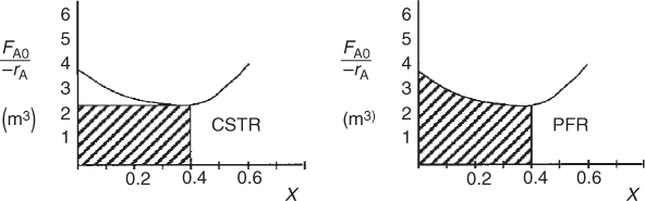
Two levenspiel plots are shown. — **Figure E11-3.2** Levenspiel plots for a CSTR and a PFR.

Graphs plotting volume against conversion for a CSTR and a PFR are shown. In both the graphs, the vertical axis represents F subscript A0 over negative r subscript A (in meter cubed) and ranges from 1 to 6 in increments of 1. The horizontal axis represents conversion X and ranges from 0 to 0.7 in increments of 0.1. For both the graphs, the curve plotted is concave upward and starts at (0,3.8) and has a minimum value at X equals 0.4. The volume for PFR is considered as the area under the curve but the volume for CSTR is taken as a rectangular portion with area lesser than that of PFR. The area is considered between conversion, X equals 0 to 0.4. The rectangular region for CSTR lies between X equals 0 to 0.4, and 0 to 2.3 meter cubed. Note: All values taken are approximate.

The PFR area (volume) is greater than the CSTR area (volume).

In this example, the adiabatic CSTR volume is less than the PFR volume.

Analysis: In this example we applied the CRE algorithm to a reversible-first-order reaction carried out adiabatically in a PFR and in a CSTR. We note that at the CSTR volume necessary to achieve 40% conversion is smaller than the volume to achieve the same conversion in a PFR. In Figure E11-3.1(c) we also see that at a PFR volume of about 3.5 m³, equilibrium is essentially reached, and no further changes in temperature, reaction rate, equilibrium conversion, or conversion take place farther down the reactor.

AspenTech: Example 11-3 has also been formulated in AspenTech and this LEP can be loaded on your computer directly from the CRE Web site. Take a look and let me know what you think!

Screenshot of the software application AspenTech is shown. — The screenshot of the Aspentech application shows the menu bar that includes the following tabs. Mixers or splitters, separations, heat exchangers, columns, reactors, pressure changers, manipulators, solids, user models, and retired. The tab reactor is selected. Icons such as R Stoic, RYield, REquil, RGibbs, RCSTR, RPlug, and RBatch are displayed under this tab. A Dropdown is provided for each of the options. Material streams are provided at the left of the screenshot.

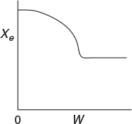
11.5 Adiabatic Equilibrium Conversion

The highest conversion that can be achieved in reversible reactions is the equilibrium conversion. For endothermic reactions, the equilibrium conversion increases with increasing temperature up to a maximum of 1.0. For exothermic reactions, the equilibrium conversion decreases with increasing temperature.

For reversible reactions, the equilibrium conversion, X_e, is usually calculated first.

11.5.1 Equilibrium Conversion

Exothermic Reactions. Figure 11-3(a) shows the variation of the concentration equilibrium constant, K_C as a function of temperature for an exothermic reaction (see Appendix C), and Figure 11-3(b) shows the corresponding equilibrium conversion X_e as a function of temperature. In Example 11-3, we saw that for a first-order reaction, the equilibrium conversion could be calculated using Equation (E11-3.12)

$\begin{matrix} X_{e} = \frac{K_{c}}{1 + K_{c}} & (E11-3.12) \end{matrix}$

First-order reversible reaction

The equilibrium conversion, X_e can be calculated as a function of temperature directly either by using Equation (E11-3.12) or from a plot of Equation (E11-3.12) such as that as shown in Figure 11-3(b).

For exothermic reactions, the equilibrium conversion decreases with increasing temperature.

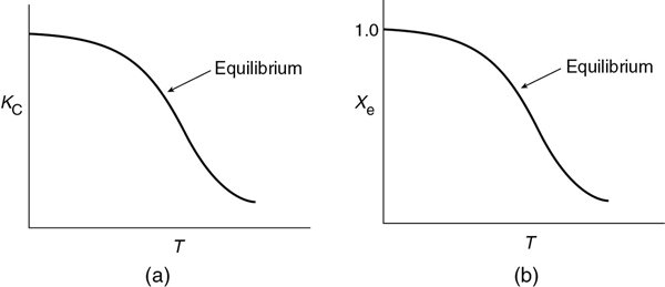
Two graphs compare the equilibrium constant and conversion with the temperature. — **Figure 11-3** Variation of equilibrium constant and conversion with temperature for an exothermic reaction (*http://www.umich.edu/~elements/6e/11chap/summary-biovan.html*).

Graph (a) compares the equilibrium constant K subscript C, and temperature T. Initially, the equilibrium constant is at a higher value. As the temperature increases, the constant K subscript C decreases. The decreasing curve is labeled as 'equilibrium'. Graph (b) compares the equilibrium conversion, X subscript e, and temperature T. Initially, the equilibrium conversion is 1.0. As the temperature increases, the conversion X subscript e gradually decreases. The decreasing curve is labeled as 'equilibrium'.

We note that the shape of the X_e versus T curve in Figure 11-3(b) will be similar for reactions that are other than first order.

To determine the maximum conversion that can be achieved in an exothermic reaction carried out adiabatically, we find the intersection of the equilibrium conversion as a function of temperature (Figure 11-3(b)) with temperature–conversion relationships from the energy balance (Figure 11-2 and Equation (T11-1.A)), as shown in Figure 11-4.

$\begin{matrix} X_{E B} = \frac{Σ Θ_{i} C_{P_{i}} (T - T_{0})}{- Δ H_{R x} (T)} & (T11-1.A) \end{matrix}$

A graph depicts the equilibrium conversion equation and the energy balance equation. — **Figure 11-4** Graphical solution of equilibrium and energy balance equations to obtain the adiabatic temperature and the adiabatic equilibrium conversion X_e.

The graph plots the conversion X, versus the temperature T. Initially, the conversion is 1.0. As the temperature increases, the conversion decreases. The decreasing curve is labeled as the equilibrium conversion equation (E11-3.12). The initial temperature is marked as the entering temperature, T subscript 0. The energy balance equation is represented as an increasing diagonal that starts at T subscript 0 and passes through the decreasing curve at a point. The vertical coordinate of this point is labeled as X subscript e. The horizontal coordinate of this point is labeled as adiabatic temperature. The energy balance equation for a higher temperature, T subscript 01 is depicted using a dashed line. It is an increasing line that passes down the curve. This line is marked as T subscript 01 is greater than T subscript 01.

Adiabatic equilibrium conversion for exothermic reactions

This intersection of the energy balance line, X_EB, with the thermodynamic equilibrium X_e curve gives the adiabatic-equilibrium conversion X_e and temperature for an entering temperature T₀ as shown in Figure 11-4.

If the entering temperature is increased from T₀ to T₀₁, the energy balance line will be shifted to the right and be parallel to the original line, as shown by the dashed line. Note that as the inlet temperature increases, the adiabatic equilibrium conversion decreases.

Example 11–4 Calculating the Adiabatic Equilibrium Temperature and Conversion

For the elementary liquid-phase reaction

A ⇄ B

we want to make a plot of equilibrium conversion as a function of temperature. The reacting species in this industrially important reaction to Jofostan’s economy have been coded with the letters A and B for reasons of National Security and for the company’s proprietary reasons.

Combine the rate law and stoichiometry to write –r_A as a function of k, C_A0, X, and X_e.
Determine the adiabatic equilibrium temperature and conversion when species A and inert I are fed to the reactor at a temperature of 480 K.
What is the CSTR volume necessary to achieve 90% of the adiabatic equilibrium conversion for C_A0 = 1.0 mol/dm³ and υ =₀ = 5 dm³/min?

Additional information:^†

$\begin{matrix} \begin{matrix} H_{A}^{o} (298 K) = - 46, 000 cal/mol & H_{B}^{o} (298 K) = - 60, 000 cal/mol \end{matrix} \\ C_{P_{I}} = 50 c a l / m o l \cdot K, C_{P_{A}} = 25 c a l / m o l \cdot K, C_{P_{B}} = 25 c a l / m o l \cdot K, Θ_{I} = 1 \\ k = 0.0 00035 \exp (\frac{E}{R} (\frac{1}{298} - \frac{1}{T}) \min^{- 1}) with E = 10000 \frac{cal}{mol} \\ K_{e} = 75000 at 298 K \end{matrix}$

^†Jofostan Journal of Thermodynamic Data, Vol. 23, p. 74 (1999).

Solution

Combine rate law and stoichiometry to write -r_A as a function of X

Mole Balance:

$\frac{d X}{d V} = - r_{A} / F_{A0} (E 11–4.1)$
Rate Law:

$- r_{A} = k (C_{A} - \frac{C_{B}}{K_{e}}) (E 11 - 4.2)$
Stoichiometry: Liquid (υ = υ₀)

We follow the algorithm given in Table 11-2 except we apply it to a liquid-phase reaction in this case so that the concentrations are written as

$\begin{matrix} C_{A} = C_{A0} (1 - X) & (E 11–4.3) \end{matrix}$

$\begin{matrix} C_{B} = C_{A 0} X & (E 11–4.4) \end{matrix}$

$\begin{matrix} - r_{A} = k C_{A 0} (1 - X - \frac{X}{K_{e}}) & \begin{matrix} (E 11–4.5) \end{matrix} \end{matrix}$

At equilibrium: -r_A = 0; so

$\begin{matrix} X_{e} = \frac{C_{A0} X_{e}}{C_{A0} (1 - X_{e})} = \frac{X_{e}}{(1 - X_{e})} & \begin{matrix} (E 11–4.6) \end{matrix} \end{matrix}$

Substituting for K_e in terms of X_e in Equation (E11-4.5) and simplifying

$\begin{matrix} - r_{A} = k C_{A0} (1 - \frac{X}{X_{e}}) \end{matrix} \begin{matrix} (E11-4.7) \end{matrix}$

Solving Equation (E11-4.6) for X_e gives

$\begin{matrix} X_{e} = \frac{K_{e} (T)}{1 + K_{e} (T)} \end{matrix} \begin{matrix} (E11-4.8) \end{matrix}$

(b) Find adiabatic equilibrium temperature and conversion
Equilibrium Constant: Calculate ΔC_P, then K_e(T) as a function of temperature

ΔC_P = C_{P_B} – C_{P_A} = 25 – 25 = 0 cal/mol · K

For ΔC_P = 0, the equilibrium constant varies with temperature according to the van’t Hoff relation

$\begin{matrix} K_{e} (T) = K_{e} (T_{1}) \exp [\frac{Δ H_{R x}^{o}}{R} (\frac{1}{T_{1}} - \frac{1}{T})] & \begin{matrix} (E 11–4.9) \end{matrix} \end{matrix}$

$\begin{matrix} \begin{array}{l} Δ H_{Rx}^{ο} = H_{B}^{ο} - H_{A}^{ο} = - 14000 cal/mol \\ K_{e} (T) = 75000 exp [\frac{- 14000}{1.987} (\frac{1}{298} - \frac{1}{T})] \\ K_{e} = 75000 \exp [- 23.64 (\frac{T - 298}{T})] \end{array} & \begin{matrix} (E 11–4.10) \end{matrix} \end{matrix}$

Substituting Equation (E11-4.10) into (E11-4.8), we can calculate the equilibrium conversion as a function of temperature:

Equilibrium Conversion from Thermodynamics:

$\begin{matrix} X_{e} = \frac{75000 exp [- 23.64 (T - 298) / T]}{1 + 75000 exp [- 23.6 4 (T - 298) / T]} \end{matrix} \begin{matrix} (E11-4.11) \end{matrix}$

We will use the tutorial in the Chapter 11 LEP “X_e vs. T” on the Web site to generate a figure of the equilibrium conversion as a function of temperature. We do this by “fooling” Polymath by using a dummy independent variable “t” to generate X_e and X_EB. Next we change variables in the plotting program to make T the independent variable and X_e and X_EB the dependent variables to obtain Figure E11-4.1. See tutorial (http://www.umich.edu/~elements/6e/software/Polymath_fooling_tutorial.pdf).

The calculations are shown in Table E11-4.1.

TABLE E11-4.1 EQUILIBRIUM CONVERSION AS A FUNCTION OF TEMPERATURE

T(K)	K_e	X_e	k (min^-1)
298	75,000.00	1.00	0.000035
350	2236.08	1.00	0.000430
400	180.57	0.99	0.002596
450	25.51	0.96	0.010507
500	5.33	0.84	0.032152
550	1.48	0.60	0.080279
620	0.35	0.26	0.225566

Note in this case the equilibrium constant K_e decreases by a factor of 10⁵ and the reaction rate constant k increases by a factor of 10⁴.

Energy Balance:

For a reaction carried out adiabatically, the energy balance, Equation (T11-1.A), reduces to

$\begin{matrix} X_{E B} = \frac{Σ Θ_{i} C_{P_{i}} (T - T_{0})}{- Δ H_{R x}} = \frac{(C_{P_{A}} + Θ_{I} C_{P_{I}}) (T - T_{0})}{- Δ H_{R x}^{o}} \end{matrix} \begin{matrix} (E 11-4.12) \end{matrix}$

$\begin{matrix} X_{EB} = \frac{75 (T - 480)}{14000} = 5.36 x 10^{- 3} (T - 480) \end{matrix} \begin{matrix} (E11-4.13) \end{matrix}$

Conversion calculated from energy balance

Data from Table E11-4.1 and the following data are plotted in Figure E11-4.1.

T(K)

480

525

575

620

X_EB

0

0.24

0.51

0.75

Figure E11-4.1 Finding the adiabatic equilibrium temperature (T_e) and conversion (X_e). Note: Curve uses approximate interpolated points.

The graph compares the values of conversion, X subscript e, and temperature, T (in Kelvin). The horizontal axis represents the values of temperature T (in Kelvin) and ranges from 350 to 850 in increments of 50. The vertical axis represents the values of adiabatic equilibrium conversion, X subscript e and ranges from 0 to 1.0 in increments of 0.1. Initially, the conversion is 1.0. As the temperature increases the conversion decreases. The decreasing curve is labeled as X subscript e. The energy balance (X subscript EB) values for a few temperatures are also plotted. The entering temperature is 480K. The values of temperature and the corresponding energy balance are as follows: (480, 0), (525, 0.24), and (572, 0.49). The increasing line joining these points intersects the decreasing curve at the point (572, 0.49). Note: all values are approximate.

Adiabatic equilibrium conversion and temperature

The intersection of X_EB(T) and X_e(T) gives X_e= 0.49 and T_e = 572 K.

(C) Calculate the CSTR volume to achieve 90% of the adiabatic equilibrium conversion corresponding to an entering temperature of 480 K

$\begin{matrix} V = \frac{F_{A 0} X}{- r_{A}} = \frac{C_{A 0} υ_{0} X}{k C_{A 0} (1 - \frac{X}{X_{e}})} = \frac{υ_{0} X}{k (1 - \frac{X}{X_{e}})} & \begin{matrix} (E 11–4.14) \end{matrix} \end{matrix}$

$\begin{matrix} k = (3.5 \times 1 0^{- 5} \exp [\frac{10000}{1. 987} (\frac{1}{298} - \frac{1}{T})]) = 3.5 \times 1 0^{- 5} \exp [16.89 (\frac{T - 298}{T})] & \begin{matrix} (E 11–4.15) \end{matrix} \end{matrix}$

From Figure E11-4.1 we see that for a feed temperature of 480 K, the adiabatic equilibrium temperature is 572 K and the corresponding adiabatic equilibrium conversion is only X_e = 0.49. For X = 0.9 X_e, the exit conversion is

X = 0.9 X_e = 0.9(0.49) = 0.44

From the adiabatic energy balance, the temperature corresponding to X = 0.44 is

$\begin{matrix} T = T_{0} + (\frac{- Δ H_{R x}}{C_{P_{A}} + C_{P_{I}}}) X = 480 K + \frac{14000}{75 \frac{c a l}{m o l K}} \frac{c a l}{m o l} (0.4 4) = 562 K (E 11 - 4.16) \end{matrix}$

T = 562 K

Now calculate V, for T = 562 K, X_e = 0.53, and k = 0.098 min^-1

$\begin{matrix} V = \frac{(0.44) (5 \frac{{dm}^{3}}{\min})}{0.098 {min}^{- 1} (1 - \frac{0.44}{0.53})} = 132.2 {dm}^{3} \end{matrix} \begin{matrix} (E11-4.17) \end{matrix}$

The molar flow rates will not affect the value of the equilibrium conversion!!

Analysis: The purpose of this example is to introduce the concept of the adiabatic equilibrium conversion and temperature. The adiabatic equilibrium conversion, X_e, is one of the first things to determine when carrying out an analysis involving reversible reactions. It is the maximum conversion one can achieve for a given entering temperature, T₀, and feed composition. If X_e is too low to be economical, try lowering the feed temperature and/or adding inerts. From Equation (E11-4.6), we observe that changing the flow rate has no effect on the equilibrium conversion. For exothermic reactions, the adiabatic conversion decreases with increasing entering temperature T₀, and for endothermic reactions the conversion increases with increasing entering T₀. One can easily generate Figure E11-4.1 using Polymath with Equations (E11-4.5) and (E11-4.7).

If adding inerts or lowering the entering temperature is not feasible, then one should consider reactor staging.

11.6 Reactor Staging with Interstage Cooling or Heating

11.6.1 Exothermic Reactions

Conversions higher than those shown in Figure E11-4.1 can be achieved for adiabatic operations by connecting reactors in series with interstage cooling.

A figure shows a series of reactors and heat exchangers. — **Figure 11-5** Reactor in series with interstage cooling.

The figure shows three reactors and two heat exchangers connected in series. The order of the series connection is as follows. The first reactor, first heat changer, second reactor, second heat exchanger, and third reactor. The entry and exit temperatures of the first reactor are marked as 500 degrees Kelvin and 800 degrees Kelvin respectively. The reactor conversion is labeled as X1. The entry and exit temperatures of the first heat exchanger are marked as 800 degrees Kelvin and 500 degrees Kelvin. The entry and exit temperatures of the second reactor are marked as 500 degrees Kelvin and 700 degrees Kelvin respectively. The reactor conversion is marked as X2. The entry and exit temperatures of the second heat exchanger are marked as 700 degrees Kelvin and 500 degrees Kelvin respectively. The entry and exit temperatures of the third reactor are marked as 500 degrees Kelvin and 570 degrees Kelvin respectively. The third reactor conversion rate is X3.

In Figure 11-5, we show the case of an exothermic adiabatic reaction taking place in a PBR reactor train. The exit temperature from Reactor 1 is very high, 800 K, and the equilibrium conversion, X_e, is low as is the reactor conversion X₁, which approaches X_e. Next, we pass the exit stream from adiabatic reactor 1 through a heat exchanger to lower the temperature back to 500 K where X_e is high but X is still low. To increase the conversion, the stream then enters adiabatic reactor 2 where the conversion increases to X₂, which is followed by a heat exchanger and the process is repeated.

The conversion–temperature plot for this scheme is shown in Figure 11-6. We see that with three interstage coolers, 88% conversion can be achieved, compared to an equilibrium conversion of 35% for no interstage cooling.

11.6.2 Endothermic Reactions

Typical values for gasoline composition

Another example of the need for interstage heat transfer in a series of reactors can be found when upgrading the octane number of gasoline. The more compact the hydrocarbon molecule for a given number of carbon atoms is, the higher the octane rating (see Section 10.3.5). Consequently, it is desirable to convert straight-chain hydrocarbons to branched isomers, naphthenes, and aromatics. The reaction sequence is

Interstage cooling used for exothermic reversible reactions

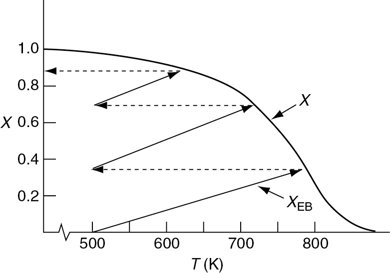
A graphic compares the values of conversion and temperature for an exothermic reaction. — **Figure 11-6** Increasing conversion by interstage cooling for an exothermic reaction. *Note:* Lines and curves are approximate.

The graph compares the values of conversion, X, and temperature T (in Kelvin). The vertical axis represents the conversion and ranges from 0 to 1.0 in increments of 0.2. The horizontal axis represents the temperature T (in kelvin) and ranges from 500 to 800 in increments of 100. A kink is present between 0 and 500 to indicate that the horizontal axis does not start from 0. As the temperature increases, the conversion decreases. The decreasing curve is labeled as X subscript e. The following three dotted lines are drawn at three conversion values. The first dotted line is drawn between a temperature of 0K to 620 K at a conversion value of 0.9. The second dotted line is drawn between a temperature of 500K to 720 K at a conversion value of 0.7. The third dotted line is drawn between a temperature of 500K to 770 K at a conversion value of 0.3. Three lines connect these dotted lines in a zig-zag manner. The first line connects the point (500, 0) and (770, 0.3). The second line connects the points (500, 0.3) and (720, 0.7) of the third and second dotted lines respectively. The third line connects the points (500, 0.9) and (600, 0.9) of the second and third dotted lines respectively. These lines are labeled as X subscript EB.

Gasoline
C₅	10%
C6	10%
C7	20%
C8	25%
C9	20%
C10	10%
C₁₁-C₁₂	5%

The first reaction step (k₁) is slow compared to the second step, and each step is highly endothermic. The allowable temperature range for which this reaction can be carried out is quite narrow: Above 530°C undesirable side reactions occur, and below 430°C the reaction virtually does not take place to any reasonable extent due to the slow reaction kinetics. A typical feed stock might consist of 75% straight chains, 15% naphthas, and 10% aromatics.

One arrangement currently used to carry out these reactions is shown in Figure 11-7. Note that the reactors are not all the same size. Typical sizes are on the order of 10–20 m high and 2–5 m in diameter. A typical feed rate of gasoline is approximately 200 m³/h at 2 atm. Hydrogen is usually separated from the product stream and recycled.

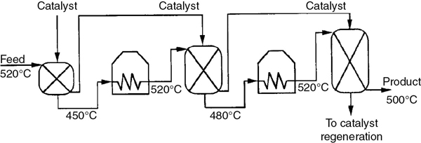
A figure shows the process of the production of gasoline. — **Figure 11-7** Interstage heating for gasoline production in moving-bed reactors.

The figure shows a series of reactors and interstage heating. The reactors are provided with catalysts. An input feed of 520 degrees celsius is passed through a catalyst coupled reactor. The temperature of the output feed from this reactor is 450 degrees celsius. This feed is passed through interstage heating to yield a feed of temperature, 520 degrees celsius. The output feed is passed onto another catalyst coupled reactor. The output from the first catalyst coupled reactor is supplied to the second one. The second catalyst coupled reactor is larger than the first catalyst coupled reactor. The temperature of the output feed from this reactor is 480 degrees celsius. This feed is passed through another interstage heating which yields an output of 520 degrees celsius. The output feed from this heating element is passed onto the third and final catalyst coupled reactor. The output from the second catalyst coupled reactor is supplied to the third one. The third catalyst coupled reactor is larger than the second catalyst coupled reactor. The temperature of the output product from this reactor is 500 degrees celsius. The output from this reactor is passed along for catalyst regeneration.

Summer 2019 $2.85/gal for octane number (ON) ON = 89

Because the reaction is endothermic, the equilibrium conversion increases with increasing temperature. A typical equilibrium curve and temperature conversion trajectory for the reactor sequence are shown in Figure 11-8.

Interstage heating

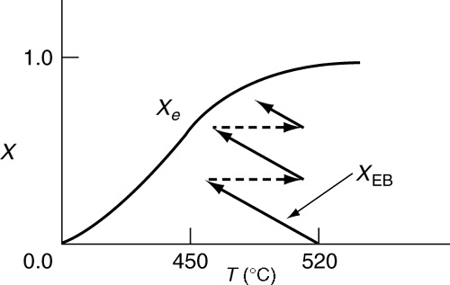
A graph plots the curves of the adiabatic equilibrium conversion and the energy balance. — **Figure 11-8** Temperature–conversion trajectory for interstage heating of an endothermic reaction analogous to Figure 11-6.

The graph compares the values of Conversion, X, and temperature (degree celsius). As the temperature increases the conversion increases. The conversion reaches a maximum of 0.9 at 520 degrees celsius. Two dashed horizontal lines are drawn at X values of 0.4 and 0.6 between a temperature of 470 degrees Celsius and 500 degrees celsius. The energy balance line, X subscript EB, runs from the point (520, 0) to the start of the first dotted line at (470, 0.4). Another energy balance line runs from the end of the first dashed line at (500, 0.4) to the start of the second dotted line at (470, 0.6). Another energy balance line projects upward from the end of the second dotted line (500, 0.6). Note: all values are approximate.

Example 11–5 Interstage Cooling for Highly Exothermic Reactions

What conversion could be achieved in Example 11-4 if two interstage coolers that had the capacity to cool the exit stream to 480 K were available? Next, determine the heat duty of each exchanger for a molar feed rate of A of 40 mol/s. Assume that 95% of the equilibrium conversion is achieved in each reactor. The feed temperature to the first reactor is 480 K.

Solution

Calculate Exit Temperature

For the reaction in Example 11-4, that is,

A ⇄ B

we saw that for an entering temperature of 480 K, the adiabatic equilibrium conversion was 0.49. For 95% of the equilibrium conversion (X_e = 0.49), the conversion exiting the first reactor is 0.47.

$\begin{matrix} X_{e} = \frac{K_{e} (T)}{1 + K_{e} (T)} \end{matrix} \begin{matrix} (E11-4.8) \end{matrix}$

$\begin{matrix} X_{e} = \frac{Σ Θ_{i} C_{P_{i}} (T - T_{0})}{- Δ H_{Rx}} = \frac{(C_{P_{A}} + Θ_{I} C_{P_{I}}) (T - T_{0})}{- Δ H_{Rx}^{\circ}} \end{matrix} \begin{matrix} (E11-4.12) \end{matrix}$

The exit temperature is found from a rearrangement of Equation (E11-4.12)

$\begin{array}{l} T = T_{0} + (\frac{- Δ H_{R x} X}{C_{P_{A}} + Θ_{I} C_{P_{I}}}) = 480 + \frac{14, 000 X}{25 + 50} = 480 + (1 86.7) (0.4 7) (E 11 - 5.1) \end{array}$

T = 568 K Answer

We will now cool the gas stream exiting the reactor at T₁ = 568 K back down to T₂ = T₀ = 480 K in a heat exchanger (Figure E11-5.1).
Calculate the Heat Load on the Heat Exchanger

The following calculations may be familiar from your course in Heat Transfer. There is no work done on the reaction gas mixture in the exchanger, and the reaction does not take place in the exchanger. Under these conditions $(F_{i | in} = F_{i | out})$ , the energy balance given by Equation (11-10)

$\ddot{Q} - {\ddot{W}}_{s} + Σ F_{i 0} H_{i 0} - Σ F_{i} H_{i} = 0 (11 - 10)$

for $\dot{W}$ _s = 0 becomes

$\ddot{Q} = Σ F_{i} H_{i} - Σ F_{i 0} H_{i 0} = Σ F_{i 0} (H_{i} - H_{i 0}) (E 11 - 5.2)$

Energy balance on the reaction gas mixture in the heat exchanger

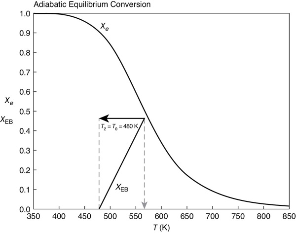
Figure E11-5.1 Reaching 95% of adiabatic equilibrium conversion, that is, X = 0.47, and then cooling back down to 480 K.

The graph compares the values of adiabatic equilibrium conversion, X subscript e, and temperature T (in Kelvin). The horizontal axis represents the temperature and ranges from 350 to 850 in increments of 50. The vertical axis represents the adiabatic equilibrium conversion, X subscript e, and ranges from 0 to 1.0 in increments of 0.1. As the temperature increases, the conversion decreases. The conversion drops to zero at 850K. A line runs from the point, (480, 0) to the point (570, 0.47). This line proceeds from the point (570, 0.47) to the point (480, 0.47). This indicates the temperature cooling from 570 K to 480 K at a conversion of 0.47. This line is labeled as X subscript EB. T2 equals T0 equals 480K. X subscript EB value is marked at 0.47. Note: all values are approximate.

$= Σ F_{i} C_{P_{i}} (T_{2} - T_{1}) = (F_{A} C_{P_{A}} + F_{B} C_{P_{B}} + F_{i} C_{P_{i}}) (T_{2} - T_{1}) (E11-5.3)$

But C_{P_A} = C_{P_B}

$\ddot{Q} = ((F_{A} + F_{B}) C_{P_{A}} + F_{I} C_{P_{I}}) (T_{2} - T_{1}) (E 11 - 5.4)$

Also, for this example, F_A0 = F_A = F_B

$\begin{array}{l} \ddot{Q} = F_{A 0} (C_{P_{A}} + C_{I} Θ_{P_{I}}) (T_{2} - T_{1}) \\ = \frac{40 mol}{s} \cdot \frac{75 cal}{mol \cdot K} (480 - 568) K \\ = - 264 \frac{kcal}{s} (E11-5.5) \end{array}$

Answer

That is, 264 kcal/s must be removed to cool the reacting mixture from 568 K to 480 K for a feed rate of 40 mol/s.
Second Reactor

Now let’s return to determine the conversion in the second reactor. Rearranging Equation (E11-4.12) for the second reactor

$\begin{array}{l} T_{2} = T_{20} + Δ X (\frac{- Δ H_{R x}^{o}}{C_{P_{A}}}) \\ = 480 + 186.7 Δ X (E11-5.6) \end{array}$

The conditions entering the second reactor are T₂₀ = 480 K and X = 0.47. The energy balance starting from this point is shown in Figure E11-5.2. The corresponding adiabatic equilibrium conversion is 0.72. Ninety-five percent of the equilibrium conversion is 68.1% and the corresponding exit temperature is T = 480 = (0.68 = 0.47)186.7 = 519 K.

X = 0.9 X_e = 0.9.0.72

∴X = 0.681

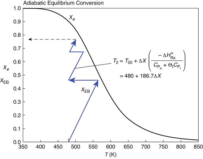
Figure E11-5.2 Three reactors in series with interstage cooling. Note: Curve uses approximate interpolated points.

The graph compares the values of adiabatic equilibrium conversion, X subscript e, and temperature T (K). The horizontal axis represents the temperature in kelvin and ranges from 350 to 850 in increments of 50. The vertical axis represents the adiabatic equilibrium conversion, X subscript e, and ranges from 0 to 1.0 in increments of 0.1. As the temperature increases, the conversion decreases. The conversion drops to zero at 850K. The temperature of the feed when passed through the first reactor changes from 480K to 570K (from the conversion of 0 to 0.47). The temperature of the feed drops from 570K to 480K as it passes through an interstage cooling. The conversion is 0.47 at interstage cooling. Further, the temperature of the feed when passed through the second reactor changes from 480K to 525K (from the conversion of 0.47 to 0.69). This temperature change is labeled as T2 equals T subscript 20 plus delta X times negative delta H degrees subscript R x over C subscript P A plus theta subscript I, C subscript P I equals 480 plus 186.7 delta X. The temperature of the feed drops from 525K to 480K as it passes through another interstage cooling. The conversion is 0.69 at this interstage cooling. Finally, the temperature of the feed when passed through the third reactor changes from 480K to 500K (from the conversion of 0.69 to 0.76). The change in temperature is represented by lines. These lines are labeled as X subscript EB.
Heat Load

The heat-exchange duty to cool the reacting mixture from 519 K back to 480 K can again be calculated from Equation (E11-5.5)

$\begin{array}{l} \ddot{Q} = F_{A 0} (C_{P_{A}} + Θ_{I} C_{P_{I}}) (480 - 519) = (\frac{40 m o 1}{s}) (\frac{75 c a 1}{m o l. K}) (- 39) \\ = - 117 \frac{kcal}{s} \end{array}$
Subsequent Reactors

For the third and final reactor, we begin at T₀ = 480 K and X = 0.68 and follow the line representing the equation for the energy balance along to the point of intersection with the equilibrium conversion, which is X_e = 0.82. Consequently, the final conversion achieved with three reactors and two interstage coolers is X = (0.95)(0.82) = 0.78.

Analysis: For highly exothermic, reversible reactions carried out adiabatically, reactor staging with interstage cooling can be used to obtain high conversions. One observes that the exit conversion and temperature from the first reactor are 47% and 568 K respectively, as shown by the energy balance line. The exit stream at this conversion is then cooled back down to 480 K where it enters the second reactor. In the second reactor, the overall conversion and temperature increase to 68% and 519 K. The slope of X versus T from the energy balance is the same as the first reactor. This example also showed how to calculate the heat load on each exchanger. We also note that the heat load on the third exchanger will be less than the first exchanger because the exit temperature from the second reactor (519 K) is lower than that of the first reactor (568 K). Consequently, less heat needs to be removed by the third exchanger.

A temperature conflict: High T rapid reaction but low X_e versus low T and slow reaction resulting in low X

11.7 Optimum Feed Temperature

We now consider an adiabatic reactor of fixed size or catalyst weight, and investigate what happens as the feed temperature is varied. The reaction is reversible and exothermic. At one extreme, using a very high feed temperature, the specific reaction rate will be large and the reaction will proceed rapidly, but the equilibrium conversion will be close to zero. Consequently, very little product will be formed. At the other extreme of low feed temperatures, the equilibrium conversion is high. So the question is, “Why not cool the feed to the lowest possible entering temperature, T₀?” The answer is that we know at low temperatures the rate constant k is small and it’s possible the reaction would not proceed to any reasonable extent, resulting in virtually no or little conversion. So we have these two extremes, low conversion at high temperatures due to equilibrium limitations and low conversion at low temperatures because of a small rate of reaction. Example 11-6 explores how to find the optimum temperature.

Bonding with Unit Operations and Heat Transfer

Example 11–6 Finding the Optimum Entering Temperature for Adiabatic Operation

We are going to continue the reaction we have been discussing in Examples 11-4 and 11-5.

A ⇄ B

To illustrate the concept of an optimum inlet temperature, we are going to plot the conversion profiles for different inlet temperatures for this isomerization, cf. Figures E11-6.2 and E11-6.3. We will use all the same parameter values and conditions we used in Examples 11-4 and 11-5 and only vary the entering temperature. We start by applying Equations (T11-2.1)–(T11-2.8) to a liquid system so where there is no temperature dependence in the concentration term, that is, C_A = C_A0 (1 – X). Starting with the mole balance

$\frac{d X}{d V} = \frac{- r_{A 0}}{F_{A 0}} (E11-6.1)$

we combine the mole balance, rate law, and stoichiometry equations to get

\begin{matrix} \frac{d X}{d V} = \frac{k C_{0}}{F_{A0}} (1 - X - \frac{X}{K_{e}}) \end{matrix} \begin{matrix} (E11-6.2) \end{matrix}

We next consider the energy balance for = 0

$T = T_{0} + \frac{X [- Δ H_{R x}^{o}]}{C_{P_{A}} + Θ C P_{I} I} = T_{0} + \frac{14, 000 X}{75} = T_{0} + 187 X (E11-6.3)$

$\begin{matrix} X_{e} = \frac{K_{e}}{1 + K_{e}} \end{matrix} \begin{matrix} (E11-6.4) \end{matrix}$

We will use the data and equations for X_e, k, and X_EB as given in Example E11-4.

Changing the Adiabatic Equilibrium Temperature and Conversion

Again using the values of X_e as a function of T in Table E11-4.1 and the energy balance

$\begin{matrix} X_{EB} = \frac{(C_{P_{A}} + Θ_{I} C_{P_{I}}) (T - T_{0})}{- Δ H_{Rx}} = 5.36 {X 10}^{- 3} (T - T_{0}) \end{matrix} \begin{matrix} (E11-6.5) \end{matrix}$

Figure E11-6.1 shows a plot X_e and X_EB on the same plot for different entering temperatures, that is, T₀.

We see that for an entering temperature of T₀ = 580 K, the adiabatic equilibrium conversion X_e is 0.24, and the corresponding adiabatic equilibrium temperature is 625 K. However, for an entering temperature of T₀ = 380 K, X_e is 0.75 and the corresponding adiabatic equilibrium temperature is 520 K.

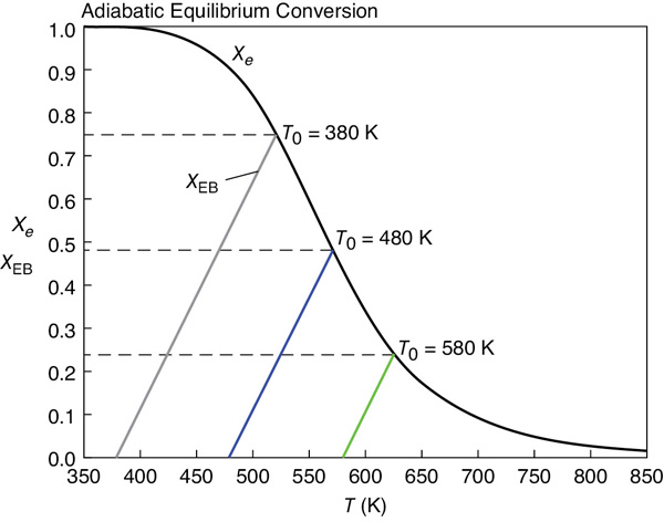
A graph shows the various values of conversion for different entering temperatures. — **Figure E11-6.1** Adiabatic equilibrium temperature.

The graph compares the values of adiabatic equilibrium conversion, X subscript e, and temperature T (in kelvin). The horizontal axis represents the temperature in kelvin and ranges from 350 to 850 in increments of 50. The vertical axis represents the adiabatic equilibrium conversion, X subscript e, and ranges from 0 to 1.0 in increments of 0.1. As the temperature increases, the conversion decreases. The conversion drops to zero at 850K. The adiabatic equilibrium conversion for entering temperatures 380K, 480K, and 580K are 0.75, 0.48, and 0.24 respectively. Lines are drawn at the three temperatures and corresponding conversion values intersecting the decreasing curve. The horizontal coordinate of the three points of intersection denotes the adiabatic equilibrium temperatures. The adiabatic equilibrium temperatures for entering temperatures 380K, 480K, and 580K are 530K, 570K, and 625K respectively.

Conversion Profiles for X and X_e

To gain insight as to why there is an optimum feed temperature, let’s look at the conversion profiles for different entering temperatures, T₀. First we enter the mole balance, rate law, stoichiometric, and energy balance equations (cf. Equations (E11-6.1)–(E11-6.5)) into Polymath, MATLAB, Python, and Wolfram. The Polymath program and output for T₀ = 480 K is shown in Table E11-6.1.

The LEP Slider icon is shown.

TABLE E11-6.1 POLYMATH PROGRAM AND NUMERICAL OUTPUT

Differential equations 1 d(X)/d(V) = –ra/Fao Explicit equations 1 k1 = 0.000035 2 T2 = 298 3 dH = -14000 4 To = 480 5 Cao = 1 6 Fao = 5 7 R = 1.987 8 E = 10000 9 Ke2 = 75000 10 T = To-dHX/(75) 11 Ke = Ke2exp((dH/R)((1/T2)-(1/T))) 12 T1 = 298 13 k = k1exp((E/R)((1/T1)-(1/T))) 14 ra = -kCao*((1-X)-(X/Ke)) 15 Xe = Ke/(1+Ke)
POLYMATH REPORT Ordinary Differential Equations Calculated values of DEQ variables
	Variable	Initial value	Final value
1	Cao	1.	1.
2	dH	-1.4E+04	-1.4E+04
3	E	10000.	10000.
4	Fao	5.	5.
5	k	0.0211 0.021138	0.1092689
6	k1	3.6e-05	3.6e-05
7	Ke	9.586656	0.9613053
8	Ke2	7.6e+04	7.6e+04
9	R	1.987	1.987
10	ra	-0.021138	-0.0027641
11	T	480.	569.1776
12	T1	298.	298.
13	T2	298.	298.
14	To	480.	480.
15	V	0	100.
16	X	0	0.477737
17	Xe	0.9055415	0.4901355

The conversion profiles for X and X_e are shown in Figure E11-6.2 for T₀ = 480 K where we see they approach each other up to the end of the 100 dm³ reactor.

Because the reactor temperature increases as we move along the reactor, the equilibrium conversion, X_e, also varies and decreases along the length of the reactor, as shown in Figure E11-6.2.

We next plot the corresponding conversion profiles down the length of the reactor for entering temperatures of 380 K, 480 K, and 580 K, as shown in Figure E11-6.3.

For an entering temperature of 580 K, we see that the conversion and temperature increase very rapidly over a short distance (i.e., a small amount of catalyst). This sharp increase is sometimes referred to as the “point” or temperature at which the

The LEP Slider icon is shown.

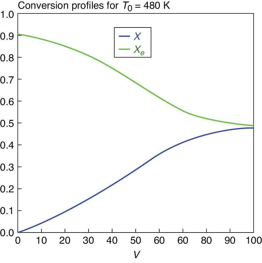
Figure E11-6.2 Conversion profiles.

A graph depicts the conversion profiles, X, and X subscript e for different feed temperatures. — **Figure E11-6.3** Equilibrium conversion for different feed temperatures.

The Graph compares the values of conversion and volume V. The horizontal axis represents the volume and ranges from 0 to 100 in increments of 10. The vertical axis represents the conversion and ranges from 0 to 1.0 in increments of 0.1. For a feed temperature of 480K, the initial conversion X is 0. As the volume increases, the conversion X increases. The conversion reaches a maximum of 0.42 at a volume of 100. At this feed temperature, the initial adiabatic equilibrium conversion, X subscript e (at volume equals 0) is 0.92. As the volume increases, the conversion X subscript e decreases. The conversion finally drops to 0.44 at volume 100. The two curves represent the X and X subscript e for feed temperature, T subscript 0 equals 480 K. For a feed temperature of 580K, the initial conversion X is 0. As the volume increases, the conversion X increases. The conversion X increases up to a value of 0.22 at a volume of 17 and stays the same up to a volume of 100. At this feed temperature, the initial adiabatic equilibrium conversion, X subscript e (at volume equals 0) is 0.49. As the volume increases, the conversion X subscript e decreases. The conversion drops to 0.22 at a volume of 17 and does not change up to a volume of 100. The two curves represent the X and X subscript e for feed temperature, T subscript 0 equals 580 K. The conversion profile, The conversion profile X subscript e does not exist for a feed temperature of 380K. For this feed temperature, the initial conversion X is 0. As the volume increases, the conversion X increases. The rate of increase is slow and minuscule. The conversion reaches a value of 0.03 at volume 100. Note: all values are approximate.

reaction “ignites.” We also observe that the conversion, which is relatively small at a value of 0.24, remains constant from V = 15 dm³ to the reactor exit. If the inlet temperature were lowered to 480 K, the corresponding equilibrium conversion would increase to 0.49; however, the reaction rate is slower at this lower temperature so that this conversion is not achieved until close to the end of the reactor. If the entering temperature were lowered further to 380 K, the corresponding equilibrium conversion would be virtually 1.0, but the rate is so slow that a conversion of 0.03 is achieved for the specified reactor volume of 100 dm³. At very low feed temperatures, the specific reaction rate will be so small that virtually all of the reactant will pass through the reactor without reacting—that is, the reaction never “ignites” and little conversion is achieved.

It is apparent that with conversions close to zero for both high and low feed temperatures, there must be an optimum feed temperature that maximizes conversion. As the feed temperature is increased from a very low value, the specific reaction rate will increase, as will the conversion. The conversion will continue to increase with increasing feed temperature until the equilibrium conversion is approached in the reaction. Further increases in feed temperature for this exothermic reaction will only decrease the conversion due to the decreasing equilibrium conversion. This optimum inlet temperature is shown in Figure E11-6.4.

If we made similar plots for other entering temperatures, we would obtain the conversion at the exit of the reactor shown in Table E11-6.2.

TABLE E11-6.2 EXIT CONVERSION AS A FUNCTION OF ENTERING TEMPERATURE

T₀	380	420	460	500	540	580	620	660
X	0.029	0.12	0.43	0.43	0.33	0.24	0.17	0.11

These exit conversions are plotted as a function of the entering temperature in Figure E11-6.4.

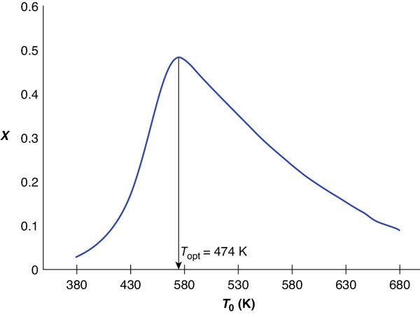
A graph derives the optimum entering temperature. — **Figure E11-6.4** Conversion at exit of reactor.

The Graph compares the values of conversion, X, and entering temperature (T subscript 0). The horizontal axis represents the temperature T subscript 0 in kelvin and ranges from 380K to 680K in increments of 50 Kelvin. The vertical axis represents the conversion and ranges from 0 to 0.6 in increments of 0.1. The initial conversion X is 0.02 at a temperature of 380K. As the temperature increases, the conversion X increases. The conversion reaches a maximum of 0.48 at a temperature of 474K. On reaching this point, the conversion starts to drop and finally reaches a value of 0.1 at a temperature of 680K. The temperature at which the conversion starts to drop is labeled as the T subscript opt. T subscript opt equals 474K.

Optimum inlet temperature

Analysis: We see that at high temperatures, the rate is rapid and equilibrium is reached near the entrance to the reactor and the conversion will be small. At the other extreme of low temperatures, the reaction never “ignites” and the reactants pass through the reactor virtually unreacted. At entering temperature between these two extremes we find there is an optimum entering feed temperature that maximizes conversion. The optimum feed temperature in this example is 474 K, and the corresponding optimum conversion is 0.48.

11.8 And Now… A Word from Our Sponsor–Safety 11 (AWFOS–S11 Acronyms)

The purpose of this tutorial is to get familiarized with commonly used acronyms in various Incident Investigation reports. Below is a list of acronyms which will be encountered frequently.

TABLE 11-4 ACRONYMS

Acronym	Meaning	Link
AIChE	American Institute of Chemical Engineers	https://www.aiche.org/about
API	American Petroleum Institute	https://www.api.org/about
BLEVE	Boiling Liquid Expanding Vapor Explosion	https://inspectapedia.com/plumbing/BLEVE-Explosions.php
CCPS	Center for Chemical Process Safety	https://www.aiche.org/ccps/about
CSB	U.S. Chemical Safety and Hazard Investigation Board	https://www.csb.gov/about-the-csb/
DCS	Distributed Control System	https://www.electricaltechnology.org/2016/08/distributed-control-system-dcs.html
EPA	Environmental Protection Agency	https://www.epa.gov/aboutepa
HAZOP	Hazard and Operability Study	https://www.oshatrain.org/notes/2bnotes21.html
HSE	Health, Safety and Environment	https://www.workplacetesting.com/definition/16/health-safety-and-environment-hse
LOPA	Layer of Protection Analysis	https://hseengineer.wordpress.com/lopa-layer-of-protection-analysis/
MOC	Management of Change	http://www.lni.wa.gov/safety/grantspartnerships/partnerships/vpp/pdfs/vppmocbestpractices.pdf
MSDS	Material Safety Data Sheet	https://www.osha.gov/Publications/OSHA3514.html
NFPA	National Fire Protection Association	https://www.nfpa.org/About-NFPA
OSHA	Occupational Safety and Health Administration	https://www.osha.gov/about.html
PPE	Personal Protective Equipment	https://www.osha.gov/SLTC/personalprotectiveequipment/
P & IDs	Piping and Instrumentation Diagrams	https://www.lucidchart.com/pages/p-and-id-discovery__top
PSSR	Pre-Startup Safety Review	https://www.chemicalprocessing.com/articles/2018/perform-a-proper-pre-startup-safety-review-5-steps/
PRVs	Pressure Relief Valves	http://www.wermac.org/valves/valves_pressure_relief.html
PHA	Process Hazard Analysis	http://www.wermac.org/valves/valves_pressure_relief.html
PSM	Process Safety Management	https://www.osha.gov/SLTC/processsafetymanagement/
RMP	Risk Management Program	https://www.osha.gov/chemicalexecutiveorder/psm_terminology.html
SIL	Safety Integrity Levels	https://www.crossco.com/blog/determining-safety-integrity-levels-sil-your-process-application
SOPs	Standard Operating Procedures	https://www.brampton.ca/EN/Business/BEC/resources/Documents/WhatisaStandardOperatingProcedure(SOP).pdf

Closure. Virtually all reactions that are carried out in industry involve heat effects. This chapter provides the basis to design reactors that operate at steady state and that involve heat effects. To model these reactors, we simply add another step to our algorithm; this step is the energy balance. One of the goals of this chapter is to understand each term of the energy balance and how it was derived. We have found that if the reader understands the various steps in the derivation, they will be in a much better position to apply the equation correctly. In order not to overwhelm the reader while studying reactions with heat effects, we have broken up the different cases and only consider the case of reactors operated adiabatically in this chapter. Chapter 12 will focus on reactors with heat exchange operated at steady state. Chapter 13 will focus on reactors not operated at steady state. An industrial adiabatic reaction concerning the manufacture of sulfuric acid that provides a number of practical details is included on the CRE Web site in PRS R12.4 (http://www.umich.edu/~elements/6e/11chap/live.html and http://www.umich.edu/~elements/6e/12chap/pdf/sulfuricacid.pdf).

The figure shows a few blocks stacked on top of each other. — The stacked blocks shown in the figure represent the topics covered in this Chapter. The topics covered (from top to bottom) are as follows. Energy balance, combine, stoichiometry, rate law, and more balance.

Summary

For the reaction

$A + \frac{b}{a} B \to \frac{c}{a} C + \frac{d}{a} D$

The heat of reaction at temperature T, per mole of A, is

$Δ H_{R x} (T) = \frac{c}{a} H_{C} (T) + \frac{d}{a} H_{D} (T) - \frac{b}{a} H_{B} (T) - H_{A} (T) (S11-1)$
The mean heat capacity difference, ΔC_P, per mole of A is

$Δ C_{P} = \frac{c}{a} C_{P C} + \frac{d}{a} C_{P D} - \frac{b}{a} C_{P B} - C_{P A} (S11-2)$

where C_{P_i} is the mean heat capacity of species i between temperatures and T_R and T.
When there are no phase changes, the heat of reaction at temperature T is related to the heat of reaction at the standard reference temperature T_R by

$Δ H_{R x} (T) = H_{R x}^{o} (T_{R}) + Δ C_{P} (T - T_{R}) (S11-3)$
The steady-state energy balance on a system volume V is

$\begin{matrix} \dot{Q} - F_{A0} Σ Θ_{i} C_{P_{i}} (T - T_{i 0}) - [Δ H_{Rx}^{\circ} (T_{R}) + Δ C_{P} (T - T_{R})] F_{A0} X = 0 \end{matrix} \begin{matrix} (S11-4) \end{matrix}$

We now couple the first four building blocks Mole Balance, Rate Law, Stoichiometry, and Combine with the fifth block, the Energy Balance, to solve nonisothermal reaction engineering problems as shown in the Closure box for this chapter.
For adiabatic operation ( $\dot{Q}$ ≡ 0) of a PFR, PBR, CSTR, or batch reactor (BR), and neglecting $\dot{W}$ _s, we solve Equation (S11-4) for the adiabatic conversion–temperature relationship, which is

$\begin{matrix} \begin{matrix} X = \frac{Σ Θ_{i} C_{P_{i}} (T - T_{0})}{- [Δ H_{Rx}^{\circ} (T_{R}) + Δ C_{p} (T - T_{R})]} \end{matrix} \end{matrix} \begin{matrix} (S11-5) \end{matrix}$

Solving Equation (S11-5) for the adiabatic temperature–conversion relationship:

$\begin{matrix} T = \frac{X [- Δ H_{Rx}^{\circ} (T_{R})] + Σ Θ_{i} C_{P_{i}} T_{0} + X Δ C_{P} T_{R}}{[Σ Θ_{i} C_{P_{i}} + X Δ C_{P}]} & (S11-6) \end{matrix}$

Using Equation (S11-4), one can solve nonisothermal adiabatic reactor problems to predict the exit conversion, concentrations, and temperature.

CRE Web Site Materials

(http://www.umich.edu/~elements/6e/11chap/obj.html#/)

Living Example Problem Formulated in AspenTech

Screenshot of the software application Aspen Plus 2006.5 is shown. — The screenshot shows the simulated process of adiabatic liquid-phase isomerization of normal butane. The process flowsheet window is displayed. This window includes a figure of the R Plug Reactor and the Heat and material balance table. Details such as stream ID, feed, and product are included in the table. The menu bar at the bottom displays various tabs such as mixers or splitters, separators, heat exchangers, columns, reactors, pressure changers, manipulators, solids, user models, and retired. The 'reactor' tab is selected. Icons for reactors such as Rstoic, R yield, RE quil, R Gibbs, RCSTR, Rplug, and RBatch are shown under this tab. A Dropdown is provided for each of the options. Material streams drop-down options are provided at the left of the screenshot.

A step-by-step AspenTech tutorial is given on the CRE Web site.
(http://www.umich.edu/~elements/6e/software/aspen.html)

Questions, Simulations, and Problems

The subscript to each of the problem numbers indicates the level of difficulty: A, least difficult; D, most difficult.

A = • B = ▪ C = ♦ D = ♦♦

An illustration of three books tied together with a rope is shown. A phrase reads, "home work problems."

In each of the questions and problems, rather than just drawing a box around your answer, write a sentence or two describing how you solved the problem, the assumptions you made, the reasonableness of your answer, what you learned, and any other facts that you want to include. See the Preface for additional generic parts (x), (y), (z) to the home problems.

Before solving the problems, state or sketch qualitatively the expected results or trends.

Questions

Q11-1_A i>clicker. Go to the Web site (http://www.umich.edu/~elements/6e/11chap/iclicker_ch11_q1.html) and view at least five i>clicker questions. Choose one that could be used as is, or a variation thereof, to be included on the next exam. You also could consider the opposite case: explaining why the question should not be on the next exam. In either case, explain your reasoning.

Q11-2_A Prepare a list of safety considerations for designing and operating chemical reactors. What would be the first four items on your list? For example, what safety concerns would you have for operating a reactor adiabatically? (See www.sache.org and www.siri.org/graphics.) The August 1985 issue of Chemical Engineering Progress may be useful.

Q11-3_A Suppose the reaction in Table 11-2 were carried out in BR instead of PFR. What steps in Table 11-2 would be different?

Q11-4_A Rework Problem P2-9_D for the case of adiabatic operation.

Q11-5_A What if you were asked to give an everyday example that demonstrates the principles discussed in this chapter? (Would sipping a teaspoon of Tabasco or other hot sauce be one?)

Q11-6_A Example 11-1: What Additional Information Is Required? How would this example change if a CSTR were used instead of a PFR?

Q11-7_A Example 11-2: Heat of Reaction. (1) What would the heat of reaction be if 50% inerts (e.g., helium) were added to the system? (2) What would be the % error if the ΔC_P term were neglected?

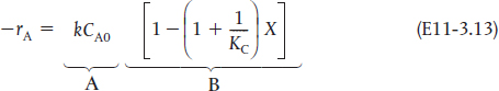
Q11-8_A Example 11-3: Adiabatic Liquid-Phase Isomerization of Normal Butane. Can you explain why the CSTR volume is smaller than the PFR volume? Hint: Equation (E11-3.13) may be helpful to your explanation.

Q11-9_A Read over the problems at the end of this chapter. Make up an original problem that uses the concepts presented in this chapter. See Problem P5-1_B for guidelines.

Q11-10_A A new energy efficiency saving device, the Turbo Retro Thermo Encabulator has been previewed in the following YouTube video (https://www.youtube.com/watch?v=RXJKdh1KZ0w). Write a two-sentence evaluation of this device that is currently on sale at a reduced introductory price.

Q11-11_A If you were to carry out a hand calculation using Simpson’s integral formula, write a step-by-step procedure to generate a table of X, T, –r_A(X), and (F_A0/–r_b). Are there any circumstances in which you would get a plot similar to the following?

Q11-12_A List three things that one should consider in the link to PPE.

Q11-13 Go to the LearnChemE screencasts link for Chapter 11 (http://www.umich.edu/~elements/6e/11chap/learn-cheme-videos.html). View one of the screencast 5- to 6-minute video tutorials and list two of the most important points.

Q11-14 AWFOS-S11 View two of the safety acronym links and write an evaluation as to whether or not the link was useful.

A graph compares the values of F subscript A0 over negative r subscript A and conversion, X. — A graph of F subscript A 0 over negative r subscript A is shown. Initially, the value of F subscript A0 over negative r subscript A is high. It gradually decreases as the values of conversion increases. This drop stops at a certain value of conversion and the values of F subscript A0 over negative r subscript A gradually increase to reach the initial value at the end. The curve formed resembles an upward parabola.

Computer Simulations and Experiments

P11-1_A Download the following programs from the CRE Web site where appropriate:

Example Table 11.2: Algorithm for Gas-Phase Reaction

Wolfram and Python
1. What happens to X and X_e profiles as you vary T₀? Can you explain this trend?
2. Use the base case for all of the variables. Which slider variable—K_e₂, k₁, or T₀—has the greatest effect on the temperature profiles? Which slider variable—E_A, F_A0, or —has the greatest effect on X and X_e?
3. Describe how the reaction rate profile changes as you vary T₀?
4. Write three conclusions on what you found in experiments (i)–(iii).
Example 11-3: Adiabatic Isomerization of Balance

Wolfram and Python
1. Describe how both X and X_e profiles change for each of the parameter values, T₀, K_C, and C_A0.
2. What is the minimum feed temperature that would give that maximum possible conversion at the end of the reactor?
3. Vary and $Δ H_{Rx}^{\circ}$ describe how the change in the temperature profile changes.
4. What parameter value—C_A0, T₀, or y_A0—affects the reaction rate profile, -r_A, the most, and in which ways does it change?
5. Write three conclusions on what you found in experiments (i)–(iv)
  
  Polymath
6. What if the butane reaction were carried out in a 0.8-m³ PFR that can be pressurized to very high pressures? What would be the conversion?
7. What inlet temperature would you recommend?
8. Is there an optimum inlet temperature?
9. Plot the heat that must be removed along the reactor ( $\dot{Q}$ vs. V) to maintain isothermal operation.
AspenTech Example 11-3. Download the AspenTech program from the CRE Web site. (1) Repeat using AspenTech. (2) Vary the inlet flow rate and temperature, and describe what you find. (3) Write three conclusions on what you found by exploring this AspenTech example.
Example 11-4: Calculating the Adiabatic Equilibrium Temperature and Conversion

Wolfram and Python
1. Go to the extremes of the ranges of the sliders and describe how the adiabatic equilibrium conversion changes with each of the variables, T, (– $Δ H_{Rx}^{\circ}$ ), K_e, and Θ_I.
2. What inlet temperatures, T₀, will give the highest and lowest values of the adiabatic equation temperature?
3. Write a set of three conclusions from your experiments (i) and (ii).
Example 11-5: Interstage Cooling for Highly Exothermic Reactions. (1) Determine the molar flow rate of cooling water (C_Pw = 18 cal/mol·K) necessary to remove 220 kcal/s from the first exchanger as shown in Figure P11-1_A (e). The cooling water enters at 270 K and leaves at 400 K. (2) Determine the necessary heat-transfer area A (m²) for an overall heat transfer coefficient, U, of 100 cal/s·m²·K. You must use the log-mean driving force in calculating $\dot{Q}$ .

$\begin{matrix} \dot{Q} = UA \frac{[(T_{h 2} - T_{c 2}) - (T_{h 1} - T_{c 1})]}{1 n (\frac{T_{h 2} - T_{c 2}}{T_{h 1} - T_{c 1}})} & (E11-5.7) \end{matrix}$

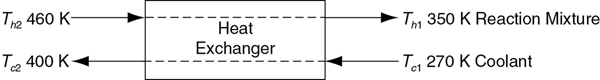
Figure P11-1_A (e) Countercurrent heat exchanger.

The figure shows a counter-current heat exchanger where the reaction mixture flows from left to right and the coolant flows from right to left. The entry (T subscript h 2) and exit (T subscript h1) temperatures of the reaction mixture feed are 460 Kelvin and 350 Kelvin respectively. The entry (T subscript c1) and exit (T subscript c2) temperatures of the coolant stream are 270 Kelvin and 400 Kelvin respectively.
Example 11-6: Optimum Feed Temperature

Wolfram and Python
1. Describe what happens to X and X_e as you increase Θ_I from 0.3 to 4.
2. Vary ΔH_Rxand describe what you find.
3. Investigate the parameters K_e, k, and Θ_I by setting each to their base case values and then vary T₀ and describe what you find.
4. Set K_e2 at its maximum value, 150,000, and then vary T₀. What differences do you observe from the base case?
5. Next set Θ_I at 3, and again vary the other parameters. Write a sentence or two saying how each variable affects the optimum feed temperature.
6. Explain how inert, Θ_I, affects the equilibrium conversion and actual conversion.
7. Write two conclusions about what you found in your experiments (i) through (vi).

The badge of the member of the hall of fame.

Problems

P11-2_A For elementary reaction

A ⇄ B

the equilibrium conversion is 0.8 at 127°C and 0.5 at 227°C. What is the heat of reaction?

P11-3_B OEQ (Old Exam Question). The equilibrium conversion is shown below as a function of catalyst weight down a PBR.

A graph compares the values of conversion and weight. — The graph compares the values of conversion, X subscript e, and weight W. Initially at W equals 0, the conversion is high. As the weight increases, the conversion gradually drops. The decrease stops at a certain weight, after which the conversion remains the same.

Please indicate which of the following statements are true and which are false. Explain each case.

The reaction could be first-order endothermic and carried out adiabatically.
The reaction is first-order endothermic and the reactor is heated along its length with T_a being constant.
The reaction is second-order exothermic and cooled along the length of the reactor with T_a being constant.
The reaction is second-order exothermic and carried out adiabatically.

P11-4_A OEQ (Old Exam Question). The elementary, irreversible, organic liquid-phase reaction

A + B → C

is carried out adiabatically in a flow reactor. An equal molar feed in A and B enters at 27°C, and the volumetric flow rate is 2 dm³/s and C_A0 = 0.1 kmol/m³.

Additional information:

$\begin{array}{l} H_{A}^{o} (273 K) = - 20 kcal/mol, H_{B}^{ο} (273 K) = - 15 kcal/mol, \\ H_{C}^{o} (273 K) = - 41 kcal/mol \end{array}$

$\begin{matrix} C_{P_{A}} = C_{P_{B}} = 15 c a l / m o l \cdot K C_{P_{C}} = 30 c a l / m o l \cdot K \\ k = 0.01 \frac{{dm}^{3}}{mol \cdot s} a t 300 K E =10,000 cal/mol \end{matrix}$

PFR

Plot and then analyze the conversion and temperature as a function of PFR volume up to where X = 0.85. Describe the trends.
What is the maximum inlet temperature one could have so that the boiling point of the liquid (550 K) would not be exceeded even for complete conversion?
Plot the heat that must be removed along the reactor ( $\dot{Q}$ vs. V) to maintain isothermal operation.
Plot and then analyze the conversion and temperature profiles up to a PFR reactor volume of 10 dm³ for the case when the reaction is reversible with K_C = 10 m³/kmol at 450 K. Plot the equilibrium conversion profile. How are the trends different than part (a)? (Ans: When V = 10 dm³ then X = 0.0051, X_eq= 0.517)

CSTR
What is the CSTR volume necessary to achieve 90% conversion?

BR
The reaction is next carried out in a 25 dm³ batch reactor charged with N_A0 = 10 moles. Plot the number of moles of A, N_A, the conversion, and the temperature as a function of time.

P11-5_A The elementary, irreversible gas-phase reaction

A → B + C

is carried out adiabatically in a PFR packed with a catalyst. Pure A enters the reactor at a volumetric flow rate of 20 dm³/s, at a pressure of 10 atm, and a temperature of 450 K.

Additional information:

$\begin{matrix} C_{P_{A}} = 40 J/mol \cdot K C_{P_{B}} = 25 J/mol \cdot K C_{P_{C}} = 15 J/mol \cdot K \\ H_{A}^{ο} = - 70 k J/mol H_{B}^{ο} = - 50 k J/mol H_{C}^{ο} = - 40 k J/mol \end{matrix}$

All heats of formation are referenced to 273 K.

$k = 0.1 33 \exp [\frac{E}{R} (\frac{1}{450} - \frac{1}{T})] \frac{d m^{3}}{k g - c a t \cdot s} with E = 31.4 k J/ m o l$

Plot and then analyze the conversion and temperature down the plug-flow reactor until an 80% conversion (if possible) is reached. (The maximum catalyst weight that can be packed into the PFR is 50 kg.) Assume that ΔP = 0.0
Vary the inlet temperature and describe what you find.
Plot the heat that must be removed along the reactor ( $\dot{Q}$ vs. V) to maintain isothermal operation.
Now take the pressure drop into account in the PBR with ρ_b = 1 kg/dm³. The reactor can be packed with one of two particle sizes. Choose one.

α = 0.019/kg-cat for particle diameter D₁

α = 0.0075/kg-cat for particle diameter D₂
Plot and then analyze the temperature, conversion, and pressure along the length of the reactor. Vary the parameters α and P₀ to learn the ranges of values in which they dramatically affect the conversion.
Apply to this problem one or more of the six ideas discussed in Table P-4 in the Complete preface-introduction on the Web site (http://www.umich.edu/~elements/6e/toc/Preface-Complete.pdf).

P11-6_B OEQ (Old Exam Question). The irreversible endothermic vapor-phase reaction follows an elementary rate law

CH₃COCH₃ → CH₂CO + CH₄

A → B + C

and is carried out adiabatically in a 500-dm³ PFR. Species A is fed to the reactor at a rate of 10 mol/min and a pressure of 2 atm. An inert stream is also fed to the reactor at 2 atm, as shown in Figure P11-6_B. The entrance temperature of both streams is 1100 K.

A figure shows an adiabatic plug-flow reactor. It shows an input stream of concentration, C subscript A 01 fed into the adiabatic PFR at a flow rate (F subscript A0) of 10 moles per minute or F subscript 10. — **Figure P11-6_B** Adiabatic PFR with inerts.

Additional information:

k = exp (34.34) – 34222/T)1/s	C_P_I 200 J/mol · K
(T in degrees Kelvin, K)
C_P_A = 700 J/mol · K	C_P_B = 90 J/mol · K
C_P_C = 80 J/mol · K	$Δ H_{Rx}^{\circ}$ = 80000 J/mol

First derive an expression for C_A01 as a function of C_A0 and Θ_I.
Sketch the conversion and temperature profiles for the case when no inerts are present. Using a dashed line, sketch the profiles when a moderate amount of inerts are added. Using a dotted line, sketch the profiles when a large amount of inerts are added. Qualitative sketches are fine. Describe the similarities and differences between the curves.
Sketch or plot and then analyze the exit conversion as a function of Θ_I. Is there a ratio of the entering molar flow rates of inerts (I) to A (i.e., Θ_I = F_I0/F_A0) at which the conversion is at a maximum? Explain why there “is” or “is not” a maximum.
What would change in parts (b) and (c) if reactions were exothermic and reversible with $Δ H_{Rx}^{\circ}$ = –80 kJ/mol and _K_C = 2 dm³/mol at 1100 K?
Sketch or plot F_B for parts (c) and (d), and describe what you find.
Plot the heat that must be removed along the reactor ( $\dot{Q}$ vs. V) to maintain isothermal operation for pure A fed and an exothermic reaction. Part (f) is “C” level of difficulty, that is, Problem P11-6_C(f).

P11-7_B OEQ (Old Exam Question). The gas-phase reversible reaction

A ⇄ B

is carried out under high pressure in a packed-bed reactor with pressure drop. The feed consists of both inerts I and Species A with the ratio of inerts to the species A being 2 to 1. The entering molar flow rate of A is 5 mol/min at a temperature of 300 K and a concentration of 2 mol/dm³. Work this problem in terms of volume. Hint:. V = W/ρ_B, r_A = ρ_Br^′_A.

Additional information:

F_A0 = 5.0 mol/min	K_C = 1000 at 300 K	T_a₀ = 300 K
C_A0 = 2 mol/dm³	C_P_B = 160 cal/mol/K	V = 40 dm³
C_I = 2C_A0	ρB = 1.2 kg/dm³	αρ_b = 0.02 dm^–3
C_FI = 18 cal/mol/K	T₀₀ = 300 K	Coolant
C_P_A = 160 cal/mol/K	T_t = 300 K	$\dot{m}$ _C = 50 mol/min
E = 10000 cal/mol	k₁ = 0.1 min^–1 at 300 K	C_P_Cool = 20 cal/mol/K
ΔH_Rx = –20000 cal/mol	Ua = 150 cal/dm³/min/K

Adiabatic Operation. Plot X, X_e, p, T, and the rate of disappearance as a function of V up to V = 40 dm³. Explain why the curves look the way they do.
Vary the ratio of inerts to A (0≤Θ_I≤10) and the entering temperature, and describe what you find.
Plot the heat that must be removed along the reactor ( $\dot{Q}$ vs. V) to maintain isothermal operation. Part (c) is “C” level of difficulty.

We will continue this problem in Chapter 12.

P11-8_B Algorithm for reaction in a PBR with heat effects

The elementary gas-phase reaction

A + B ⇄ 2C

is carried out in a packed-bed reactor. The entering molar flow rates are F_A0 = 5 mol/s, F_B0 = 2F_A0, and F_I = 2F_A0 with C_T0 = 0.3 mol/dm³. The entering temperature is 330 K.

Additional information:

$C_{P_{A}} = C_{P_{B}} = C_{P_{C}} = 20 cal/mol/ K, C_{P_{I}} = 40 cal/mol/ K, E = 25 \frac{kcal}{mol},$

$Δ H_{Rx} = - 20 \frac{kcal}{mol} @ 298 K$

$α = 0.0002 {kg}^{- 1}, k = 0.004 \frac{{dm}^{6}}{kg \cdot mol \cdot s} @ 310 K,$

K_C = 1000 @298 K

Note: This problem is continued in Problem P12-1_A with some of the entering conditions (e.g., F_B0) modified.

Write the mole balance, the rate law, K_C as a function of T, k as a function of T, and C_A, C_B, C_C as a function of X, p, and T.
Write the rate law as a function of X, p, and T.
Show the equilibrium conversion is

$X_{e} = \frac{\frac{3 K_{C}}{4} - \sqrt{(\frac{3 K_{C}}{4})^{2} - 2 K_{C} (\frac{F_{C}}{4} - 1)}}{2 (\frac{K_{C}}{4} - 1)}$

and then plot X_e versus T.
What are ΣΘ_iC_P_i, ΔC_P, T₀, entering temperature T₁ (rate law), and T₂ (equilibrium constant)?
Write the energy balance for adiabatic operation.
Case 1 Adiabatic Operation. Plot and then analyze X_e, X, p, and T versus W when the reaction is carried out adiabatically. Describe why the profiles look the way they do. Identify those terms that will be affected by inerts. Sketch what you think the profiles X_e, X, p, and T will look like before you run the Polymath program to plot the profiles. (Ans: At W = 800 kg then X = 0.3583)
Plot the heat that must be removed along the reactor ( $\dot{Q}$ vs. V) to maintain isothermal operation. Part (g) is “C” level of difficulty, that is, Problem P11-8_C(g).

P11-9_A The reaction

A + B ⇄ C + D

is carried out adiabatically in a series of staged packed-bed reactors with interstage cooling (see Figure 11-5). The lowest temperature to which the reactant stream may be cooled is 27°C. The feed is equal molar in A and B, and the catalyst weight in each reactor is sufficient to achieve 99.9% of the equilibrium conversion. The feed enters at 27°C and the reaction is carried out adiabatically. If four reactors and three coolers are available, what conversion may be achieved?

Additional information:

$Δ H_{Rx}^{\circ}$ 30000 cal/mol A	C_P_A = C_P_B = C_P_C = C_P_D = 25 cal/mol · K
K_e (50°C) = 500000	F_A0 = 10 mol A/min

First prepare a plot of equilibrium conversion as a function of temperature. (Partial ans: T = 360 K, X_e = 0.984; T = 520 K, X_e = 0.09; T = 540 K, X_e = 0.057)

P11-10_A Figure P11-10_A shows the temperature–conversion trajectory for a train of reactors with interstage heating. Now consider replacing the interstage heating with injection of the feed stream in three equal portions, as shown in Figure P11-10_A:

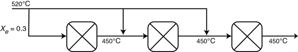
A figure shows a series of three reactors. — **Figure P11-10_A**

The figure shows an input feed of 520 degrees celsius supplied to three reactors. The three reactors are connected in series. A feed stream of 520 degrees celsius is supplied as the individual input of three reactors. The temperature of the output stream from each of these reactors is 450 degrees celsius. The adiabatic equilibrium conversion is 0.3.

Sketch the temperature–conversion trajectories for (a) an endothermic reaction with entering temperatures as shown, and (b) an exothermic reaction with the temperatures to and from the first reactor reversed, that is, T₀ = 450°C.

Supplementary Reading

An excellent development of the energy balance is presented in

R. ARIS, Elementary Chemical Reactor Analysis. Upper Saddle River, NJ: Pearson, 1969, Chaps. 3 and 6.

A number of example problems dealing with nonisothermal reactors may or may not be found in

THORNTON W. BURGESS, The Adventures of Old Man Coyote. New York: Dover Publications, Inc., 1916.

JOHN B. BUTT, Reaction Kinetics and Reactor Design, Revised and Expanded, 2nd ed. New York: Marcel Dekker, Inc., 1999.

S. M. WALAS, Chemical Reaction Engineering Handbook of Solved Problems. Amsterdam: Gordon and Breach, 1995. See the following solved problems: 4.10.1, 4.10.08, 4.10.09, 4.10.13, 4.11.02, 4.11.09, 4.11.03, 4.10.11.

For a thorough discussion on the heat of reaction and equilibrium constant, one might also consult

K. G. DENBIGH, Principles of Chemical Equilibrium, 4th ed. Cambridge: Cambridge University Press, 1981.
The heats of formation, H(T), Gibbs free energies, G_e(T_R), and the heat capacities of various compounds can be found in

D. W. GREEN, and R. H. PERRY, eds., Chemical Engineers’ Handbook, 8th ed. New York: McGraw-Hill, 2008.

R. C. REID, M. PRAUSNITZ, and T. K. SHERWOOD, The Properties of Gases and Liquids, 3rd ed. New York: McGraw-Hill, 1977.

R. C. WEAST, ed., CRC Handbook of Chemistry and Physics, 94th ed. Boca Raton, FL: CRC Press, 2013.

..................Content has been hidden....................

You can't read the all page of ebook, please click here login for view all page.

Table of Contents for 11. Nonisothermal Reactor Design: The Steady-State Energy Balance and Adiabatic PFR Applications

Create new playlist

Sign In

Sign Up

11. Nonisothermal Reactor Design: The Steady-State Energy Balance and Adiabatic PFR Applications

11.1 Rationale

11.2 The Energy Balance

11.2.1 First Law of Thermodynamics

11.2.2 Evaluating the Work Term

11.2.3 Overview of Energy Balances

11.3 The User-Friendly Energy Balance Equations

11.3.1 Dissecting the Steady-State Molar Flow Rates to Obtain the Heat of Reaction

11.3.2 Dissecting the Enthalpies

11.3.3 Relating ΔHRx(T), ΔHRxo(TR), and ΔCP

11.4 Adiabatic Operation ∴ Q˙ = 0

11.4.1 Adiabatic Energy Balance

11.4.2 Adiabatic Tubular Reactor

11.5 Adiabatic Equilibrium Conversion

11.5.1 Equilibrium Conversion

11.6 Reactor Staging with Interstage Cooling or Heating

11.6.1 Exothermic Reactions

11.6.2 Endothermic Reactions

11.7 Optimum Feed Temperature

11.8 And Now… A Word from Our Sponsor–Safety 11 (AWFOS–S11 Acronyms)

Summary

CRE Web Site Materials

Questions, Simulations, and Problems

Questions

Computer Simulations and Experiments

Problems

Supplementary Reading

Table of Contents for
11. Nonisothermal Reactor Design: The Steady-State Energy Balance and Adiabatic PFR Applications

11.3.3 Relating ΔH_Rx(T), ${Δ H}_{Rx}^{o} (T_{R})$ , and ΔC_P

11.4 Adiabatic Operation ∴ $\dot{Q}$ = 0