C. Thermodynamic Relationships Involving the Equilibrium Constant

Search in book...
Toggle Font Controls
Create new playlist

Name your new playlist

Playlist description (optional)
Sign In

Email address

Password

Forgot Password?

or

Continue with Facebook

Continue with Google
Sign Up

Full Name

Email address

Confirm Email Address

Password

or

Continue with Facebook

Continue with Google

C. Thermodynamic Relationships Involving the Equilibrium Constant¹

¹ For the limitations and for further explanation of these relationships, see, for example, K. Denbigh, The Principles of Chemical Equilibrium, 3rd ed. Cambridge: Cambridge University Press, 1971, p. 138.

For the gas-phase reaction

$\begin{matrix} A+ \frac{b}{a} B ⇄ \frac{c}{a} + \frac{d}{a} D & \begin{matrix} (2-2) \end{matrix} \end{matrix}$

The true (dimensionless) equilibrium constant

RTInK = –ΔG

$K = \frac{a_{C}^{c / a} a_{D}^{d / a}}{a_{A} a_{B}^{b / a}}$

where a_i is the activity of species i

$a_{i} = \frac{f_{i}}{f_{i}^{\circ}}$

where

f_i = fugacity of species i

$f_{i}^{\circ}$ = fugacity of species i at the standard state. For gases, the standard state is 1 bar, which is in the noise level of 1 atm, so we will use atm.

$a_{i} = \frac{f_{i}}{f_{i}^{\circ}} = γ_{i} P_{i}$

where γ_i is the activity coefficient

K = True equilibrium constant

K_γ Activity equilibrium constant

K_p = Pressure equilibrium constant

K_c = Concentration equilibrium constant

K_γ has units of [atm] ${[atm]}^{- (d / a + c / a - \frac{b}{a} - 1)} = {[atm]}^{- δ}$

K_p has units of [atm] ${[atm]}^{- (d / a + c / a - \frac{b}{a} - 1)} = {[atm]}^{δ}$

For ideal gases K_γ = 1.0 atm^–δ
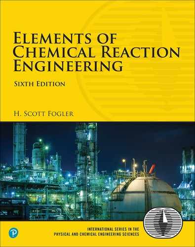
For the generic reaction (2-2), the pressure equilibrium constant K_P is

$\begin{matrix} \begin{matrix} K_{p} = & \frac{P_{C}^{c / a} P_{D}^{d / a}}{P_{A} P_{B}^{b / a}} \\ P_{i} = & partial pressure of species i, atm, k P a. \\ P_{i} = & C_{i} R T \end{matrix} & \begin{matrix} (C-1) \end{matrix} \end{matrix}$
For the generic reaction (2-2), the concentration equilibrium constant K_C is

$\begin{matrix} K_{c} = \frac{C_{C}^{c / a} C_{D}^{d / a}}{C_{A} C_{B}^{b / a}} & \begin{matrix} (C-2) \end{matrix} \end{matrix}$

It is important to be able to relate K, Kγ, K_c, and K_p.
For ideal gases, K_c and K_p are related by

$\begin{matrix} K_{p} = K_{c} {(R T)}^{δ} & \begin{matrix} (C-3) \end{matrix} \end{matrix}$

where for the generic reaction (2-2),

$\begin{matrix} δ = \frac{c}{a} + \frac{d}{a} - \frac{b}{a} - 1 & \begin{matrix} (C-4) \end{matrix} \end{matrix}$
K_P is a function of temperature only, and the temperature dependence of K_P is given by van’t Hoff’s equation:

$\begin{matrix} \begin{matrix} \frac{d {ln K}_{p}}{d T} = \frac{Δ H_{Rx} (T)}{R T^{2}} \end{matrix} & (C-5) \end{matrix}$

$\begin{matrix} \frac{d ln K_{p}}{d T} = \frac{Δ H_{Rx}^{\circ} (T_{R}) + Δ C_{P} (T - T_{R})}{{R T}^{2}} & \begin{matrix} (C-6) \end{matrix} \end{matrix}$

(http://www.umich.edu/~elements/6e/11chap/summary-biovan.html).
Integrating, we have

$\begin{matrix} ln \frac{K_{p} (T)}{K_{p} (T_{1})} = \frac{Δ H_{Rx}^{\circ} (T_{R}) - T_{R} Δ C_{p}}{R} (\frac{1}{T_{1}} - \frac{1}{T}) + \frac{Δ C_{p}}{R} ln \frac{T}{T_{1}} & \begin{matrix} (C-7) \end{matrix} \end{matrix}$

K_p and K_c are related by

$\begin{matrix} K_{c} = \frac{K_{p}}{{(R T)}^{δ}} & (C-8) \end{matrix}$

when

$δ = (\frac{d}{a} + \frac{c}{a} - \frac{b}{a} - 1) = 0$

then

K_P = K_C
K_P neglecting ΔC_P. Given the equilibrium constant at one temperature, T₁, K_P (T₁), and the heat of reaction, ${Δ H}_{Rx}^{°}$ , the partial pressure equilibrium constant at any temperature T is

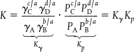
$\begin{matrix} K_{p} (T) = K_{p} (T_{1}) exp [\frac{{Δ H}_{Rx}^{°} (T_{R})}{R} (\frac{1}{T} - \frac{1}{T})] & (C-9) \end{matrix}$
From Le Châtelier’s principle we know that for exothermic reactions, the equilibrium shifts to the left (i.e., K and X_e decrease) as the temperature increases. Figures C-1 and C-2 show how the equilibrium constant varies with temperature for an exothermic reaction and for an endothermic reaction, respectively.

Figure C-1 Exothermic reaction.

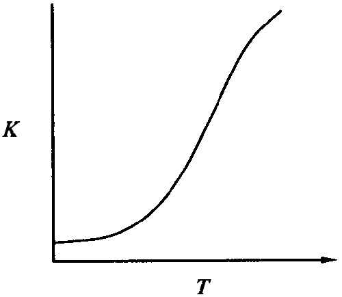
Figure C-2 Endothermic reaction.
The equilibrium constant for the reaction (2-2) at temperature T can be calculated from the change in the Gibbs free energy using

$\begin{matrix} - R T ln [K (T)] = Δ G_{Rx}^{\circ} (T) & \begin{matrix} (C-10) \end{matrix} \end{matrix}$

$\begin{matrix} ° G_{R x}^{°} = \frac{c}{a} G_{C}^{°} + \frac{d}{a} G_{D}^{°} - \frac{b}{a} G_{B}^{°} - G_{A}^{°} & (C-11) \end{matrix}$
Tables that list the standard Gibbs free energy of formation of a given species $G_{i}^{\circ}$ are available in the literature (webbook.nist.gov).
The relationship between the change in Gibbs free energy and enthalpy, H, and entropy, S, is

$\begin{matrix} Δ G = Δ H - T Δ S & (C-12) \end{matrix}$

See https://www.chm.uri.edu/weuler/chm112/lectures/lecture26.html. An example on how to calculate the equivalent conversion for ΔG is given on the Web site.

Example C–1 Water-Gas Shift Reaction

The water-gas shift reaction to produce hydrogen

H₂O + CO CO₂ ⇄CO₂ + H₂

is to be carried out at 1000 K and 10 atm. For an equimolar mixture of water and carbon monoxide, calculate the equilibrium conversion and concentration of each species.

Data: At 1000 K and 10 atm, the Gibbs free energies of formation are $G_{CO}^{\circ} = - 47, 860 cal/mol; G_{{CO}_{2}}^{\circ} = - 94, 630 cal/mol; G_{H_{2} O}^{\circ} = - 46, 040 cal/mol; and G_{H_{2}}^{\circ} = 0$ .

Solution

We first calculate the equilibrium constant. The first step in calculating K is to calculate the change in Gibbs free energy for the reaction. Applying Equation (C-10) gives us

Calculate $Δ G_{Rx}^{\circ}$

$\begin{matrix} Δ G_{Rx}^{\circ} & = & G_{H_{2}}^{\circ} + G_{{CO}_{2}}^{\circ} - G_{CO}^{\circ} - G_{H_{2} O}^{\circ} (EC-1.1) \\ = & 0 + (- 94, 630) - (- 47, 860) - (- 46, 040) \\ = & - 730 cal/mol \end{matrix}$

$\begin{matrix} \begin{matrix} - R T ln K & = & Δ G_{Rx}^{\circ} (T) \end{matrix} & (C-10) \end{matrix}$

Calculate K

$\begin{matrix} \begin{matrix} ln K & = & - \frac{Δ G_{Rx}^{\circ} (T)}{R T} = \frac{- (- 730 cal/mol)}{1.987 cal.mol \cdot K (1000 K)} \end{matrix} & (EC-1.2) \end{matrix}$

= 0.367

then

$\begin{matrix} K & = & 1.44 \end{matrix}$

Expressing the equilibrium constant first in terms of activities and then finally in terms of concentration, we have

$\begin{matrix} K = \frac{a_{{CO}_{2}} a_{H_{2}}}{a_{CO} a_{H_{2}} O} = \frac{f_{{CO}_{2}} f_{H_{2}}}{f_{CO} f_{H_{2}} O} = \frac{γ_{{CO}_{2}} P_{{CO}_{2}} γ_{H_{2}} P_{H_{2}}}{γ_{CO} P_{CO} γ_{H_{2} O} P_{H_{2} O}} & \begin{matrix} (EC-1.3) \end{matrix} \end{matrix}$

where a_i is the activity, f_i is the fugacity, =_i is the activity coefficient (which we shall take to be 1.0 owing to high temperature and low pressure), and y_i is the mole fraction of species i.² Substituting for the mole fractions in terms of partial pressures gives

$\begin{matrix} K = \frac{P_{{CO}_{2}} P_{H_{2}}}{P_{CO} P_{H_{2} O}} & \begin{matrix} (EC-1.4) \end{matrix} \end{matrix}$

$\begin{matrix} P_{i} = C_{i} R T & (EC-1.5) \end{matrix}$

$\begin{matrix} K = \frac{C_{{CO}_{2}} C_{H_{2} O}}{C_{CO} C_{H_{2} O}} & \begin{matrix} (EC-1.6) \end{matrix} \end{matrix}$

² See Chapter 17 in J. R. Elliott and C. T. Lira, Introductory Chemical Engineering Thermodynamics, 2nd ed. Upper Saddle River, NJ: Pearson, 2012, and Chapter 16 in J. W. Tester and M. Modell, Thermodynamics and Its Applications, 3rd ed. Upper Saddle River, NJ: Pearson, 1997.

Relate K and X_e.

In terms of conversion for an equimolar feed, we have

$\begin{matrix} K = \frac{C_{CO,0} X_{e} C_{CO,0} X_{e}}{C_{CO,0} (1 - X_{e}) C_{CO,0} (1 - X_{e})} & \begin{matrix} (EC-1.7) \end{matrix} \end{matrix}$

$\begin{matrix} = \frac{X^{2}}{(1 - X_{e})} = 1.44 & \begin{matrix} (EC-1.8) \end{matrix} \end{matrix}$

From Figure EC-1.1 we read at 1000 K that log K_P = 0.15; therefore, K_P = 1.41, which is close to the calculated value. We note that there is no net change in the number of moles for this reaction (i.e., ); therefore,

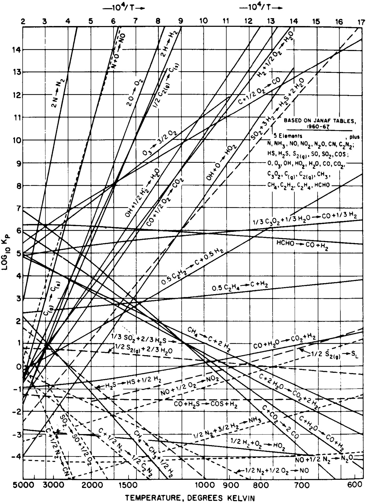
A chart marks the equilibrium constant for several chemical reactions as a function of temperature. — **Figure EC-1.1** Modell, Michael, and Reid, Robert, *Thermodynamics and Its Applications*, 2nd ed., © 1983. Reprinted and electronically reproduced by permission of Pearson Education, Inc., Upper Saddle River, NJ.

A chart mapping the chemical reaction of several elements with their equilibrium constant is shown based on JANAF tables (1960 to 1967). The temperature in degrees Kelvin is marked from 5000 to 600 Kelvin with different intervals at the bottom of the chart, the equilibrium constant is marked vertically as Log base 10 K subscript p ranges from negative 4 to 14. The values of negative 10 superscript 4 over T are marked horizontally on the top of the chart from 2 to 17. The linear lines across the axes are drawn for each reaction. Reactions with high-temperature ratio are as follows: 2 N gives N2 at (3 log base 10, 4.4); N plus O gives NO at (negative 0.8 log base 10, 6.2); 2 O gives O 2 (negative 1.8 log base 10, 8.2); 2 H gives H2 at (negative 1.5 log base 10, 9.1), OH plus 0.5 molecules of H2 gives H2O at (negative 0.9 log base 10, 12.5), and so on. Reactions with steep decrease are as follows: C plus 0.5 molecules of N 2 gives CN at (2500, 0.1), CH4 gives CH3 plus 0.5 molecules of H2 at (2.2, 1200), etcetera. Note: all values are approximate.

K = K_p = K_c (dimensionless)

Calculate X_e, the equilibrium conversion.

Taking the square root of Equation (EC-1.8) yields

$\begin{matrix} \frac{X_{e}}{1 - X_{e}} = {(1.44)}^{1 / 2} = 1.2 & \begin{matrix} (EC-1.9) \end{matrix} \end{matrix}$

Solving for X_e, we obtain

$X_{e} = \frac{1.2}{2.2} = 0.55$

Then

$\begin{matrix} \begin{matrix} C_{CO,0} & = & \frac{y_{CO,0 P_{0}}}{{R T}_{0}} \\ \begin{matrix} \begin{matrix} = \end{matrix} \\ = \end{matrix} & \frac{(0.5) (10 atm)}{(0.082 {dm}^{3} \cdot atm/mol \cdot K) (1000 K)} \end{matrix} \\ 0.061 {mol/dm}^{3} \end{matrix}$

Calculate C_CO,_e, the equilibrium conversion of CO

$\begin{array}{l} {C_{CO,e} = C_{CO,0} (1 - X_{e}) = (0.061) (1 - 0.55) = 0.0275 mol/dm}^{3} \\ {\begin{matrix} C_{H_{2}} o,e = 0.0275 mol/dm \end{matrix}}^{3} \end{array}$

${C_{CO2, e} = C_{H_{2, e}} = C_{CO,0} X_{e} = 0.0335 mol/dm}^{3}$

Figure EC-1.1 gives the equilibrium constant as a function of temperature for a number of reactions. Reactions in which the lines increase from left to right are exothermic.

The following links give thermochemical data. (Heats of Formation, C_P, etc.)

Also see Chem. Tech., 28 (3) (March), 19 (1998).

..................Content has been hidden....................

You can't read the all page of ebook, please click here login for view all page.

where	f_i = fugacity of species i
	$f_{i}^{\circ}$ = fugacity of species i at the standard state. For gases, the standard state is 1 bar, which is in the noise level of 1 atm, so we will use atm.

Table of Contents for C. Thermodynamic Relationships Involving the Equilibrium Constant

Create new playlist

Sign In

Sign Up

C. Thermodynamic Relationships Involving the Equilibrium Constant1

Table of Contents for
C. Thermodynamic Relationships Involving the Equilibrium Constant

C. Thermodynamic Relationships Involving the Equilibrium Constant¹