
LEARNING OBJECTIVES
To be aware of the major software testing techniques
To see how different test objectives lead to the selection of different testing techniques
To appreciate a classification of testing techniques, based on the objectives they try to reach
To be able to compare testing techniques with respect to their theoretical power as well as their practical value
To understand the role and contents of testing activities in different life cycle phases
To be aware of the contents and structure of the test documentation
To be able to distinguish different test stages
To be aware of some mathematical models to estimate the reliability of software
Note
Testing should not be confined to merely executing a system to see whether a given input yields the correct output. During earlier phases, intermediate products can, and should, be tested as well. Good testing is difficult. It requires careful planning and documentation. There exist a large number of test techniques. We discuss the major classes of test techniques with their characteristics.
Suppose you are asked to answer the kind of questions posed in (Baber, 1982):
Would you trust a completely automated nuclear power plant?
Would you trust a completely automated pilot whose software was written by yourself? What if it was written by one of your colleagues?
Would you dare to write an expert system to diagnose cancer? What if you are personally held liable in a case where a patient dies because of a malfunction of the software?
You will (probably) have difficulties answering all these questions in the affirmative. Why? The hardware of an airplane probably is as complex as the software for an automatic pilot. Yet, most of us board an airplane without any second thoughts.
As our society's dependence on automation increases, the quality of the systems we deliver increasingly determines the quality of our existence. We cannot hide from this responsibility. The role of automation in critical applications and the threats these applications pose should make us ponder. ACM Software Engineering Notes runs a column 'Risks to the public in computer systems' in which we are told of numerous (near-)accidents caused by software failures. The discussion on software reliability provoked by the Strategic Defense Initiative is a case in point (Parnas, 1985; Myers, 1986; Parnas, 1987). Discussions, such as those about the Therac-25 accidents or the maiden flight of the Ariane 5 (see Section 1.4), should be compulsory reading for every software engineer.
Software engineering is engineering. Engineers aim for the perfect solution, but know this goal is generally unattainable. During software construction, errors are made. To locate and fix those errors through excessive testing is a laborious affair and mostly not all the errors are found. Good testing is at least as difficult as good design.
With the current state of the art we are not able to deliver fault-free software. Different studies indicate that 30–85 errors per 1000 lines of source code are made. These figures seem not to improve over time. During testing, quite a few of those errors are found and subsequently fixed. Yet, some errors do remain undetected. Myers (1986) gives examples of extensively tested software that still contains 0.5-3 errors per 1000 lines of code. A fault in the seat-reservation system of a major airline company incurred a loss of $50 million in one quarter. The computerized system reported that cheap seats were sold out when this was, in fact, not the case. As a consequence, clients were referred to other companies. The problems were not discovered until quarterly results were found to lag considerably behind those of their competitors.
Testing is often taken to mean executing a program to see whether it produces the correct output for a given input. This involves testing the end-product, the software itself. As a consequence, the testing activity often does not get the attention it deserves. By the time the software has been written, we are often pressed for time, which does not encourage thorough testing.
Postponing test activities for too long is one of the most severe mistakes often made in software development projects. This postponement makes testing a rather costly affair. Figure 13.1 shows the results of a 1980 study by Boehm about the cost of error correction relative to the phase in which the error is discovered. This picture shows that errors which are not discovered until after the software has become operational incur costs that are 10 to 90 times higher than those of errors that are discovered during the design phase. This ratio still holds for big and critical systems (Boehm and Basili, 2001). For small, noncritical systems, the ratio may be more like 1 to 5.
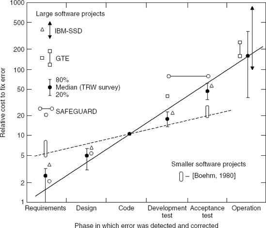
Figure 13.1. Relative cost of error correction (Source: Barry B. Boehm, Software Engineering Economics, Figure 4.2, p. 40, © 1981, Reprinted by permission of Prentice Hall, Inc. Englewood Cliffs, NJ.)
The development methods and techniques that are applied in the phases prior to implementation are least developed, relatively. It is therefore not surprising that most of the errors are made in those early phases. An early study by Boehm showed that over 60% of the errors were introduced during the design phase, as opposed to 40% during implementation (Boehm, 1975). Worse still, two-thirds of the errors introduced at the design phase were not discovered until after the software had become operational.
It is therefore incumbent on us to carefully plan our testing activities as early as possible. We should also start the actual testing activities at an early stage. An extreme form of this is test-driven development, one of the practices of XP, in which development starts with writing tests. If we do not start testing until after the implementation stage, we are really far too late. The requirements specification, design, and design specification may also be tested. The rigor with which this can be done depends on the form in which these documents are expressed. This has already been hinted at in previous chapters. In Section 13.2, we will again highlight the various verification and validation activities that may be applied at the different phases of the software life cycle. The planning and documentation of these activities is discussed in Section 13.3.
Before we decide upon a certain approach to testing, we have to determine our test objectives. If the objective is to find as many errors as possible, we will opt for a strategy which is aimed at revealing errors. If the objective is to increase our confidence in the proper functioning of the software, we may well opt for a completely different strategy. So the objective will have an impact on the test approach chosen, since the results have to be interpreted with respect to the objectives set forth. Different test objectives and the degree to which test approaches fit these objectives are the topic of Section 13.1.
Testing software shows only the presence of errors, not their absence. As such, it yields a rather negative result: up to now, only n (n ≥ 0) errors have been found. Only when the software is tested exhaustively are we certain about its functioning correctly. In practice this seldom happens. A simple program such as:
for(i = 1; i<100; i++) {if(a[i]) System.out.println("1");elseSystem.out.println("0"); };
has 2100 different outcomes. Even on a very fast machine — say a machine which executes 10 million print instructions per second — exhaustively testing this program would take 3 × 10¹⁴ years.
An alternative to this brute force approach to testing is to prove the correctness of the software. Proving the correctness of software very soon becomes a tiresome activity, however. It furthermore applies only in circumstances where software requirements are stated formally. Whether these formal requirements are themselves correct has to be decided upon in a different way.
We are thus forced to make a choice. It is of paramount importance to choose a sufficiently small, yet adequate, set of test cases. Test techniques may be classified according to the criterion used to measure the adequacy of a set of test cases:
Coverage-based testing Testing requirements are specified in terms of the coverage of the product (program, requirements document, etc.) to be tested. For example, we may specify that all statements of the program should be executed at least once if we run the complete test set, or that all elementary requirements from the requirements specification should be exercised at least once.
Fault-based testing Testing requirements focus on detecting faults. The fault-detecting ability of the test set then determines its adequacy. For example, we may artificially seed a number of faults in a program, and then require that a test set reveal at least, say, 95% of these artificial faults.
Error-based testing Testing requirements focus on error-prone points, based on knowledge of the typical errors that people make. For example, off-by-1 errors are often made at boundary values such as 0 or the maximum number of elements in a list, and we may specifically aim our testing effort at these boundary points.
Alternatively, we may classify test techniques based on the source of information used to derive test cases:
Black-box testing, also called functional or specification-based testing: test cases are derived from the specification of the software, i.e. we do not consider implementation details.
White-box testing, also called structural or program-based testing: a complementary approach, in which we do consider the internal logical structure of the software in the derivation of test cases.
We will use the first classification and discuss different techniques for coverage-based, fault-based, and error-based testing in Sections 13.5 to 13.7. These techniques involve the actual execution of a program. Manual techniques which do not involve program execution, such as code reading and inspections, are discussed in Section 13.4. In Section 13.8 we assess some empirical and theoretical studies that aim to put these different test techniques in perspective.
The above techniques are applied mainly at the component level. This level of testing is often done concurrently with the implementation phase. It is also called unit testing. Besides the component level, we also have to test the integration of a set of components into a system. Possibly also, the final system will be tested once more under direct supervision of the prospective user. In Section 13.9, we will sketch these different test phases.
At the system level, the goal pursued often shifts from detecting faults to building trust, by quantitatively assessing reliability. Software reliability is discussed in Section 13.10.
Until now, we have not been very precise in our use of the notion of an 'error'. In order to appreciate the following discussion, it is important to make a careful distinction between the notions error, fault, and failure. An error is a human action that produces an incorrect result. The consequence of an error is software containing a fault. A fault thus is the manifestation of an error. If encountered, a fault may result in a failure.[22]
So, what we observe during testing are failures. These failures are caused by faults, which are in turn the result of human errors. A failure may be caused by more than one fault and a fault may cause different failures. Similarly, the relation between errors and faults need not be 1–1.
One possible aim of testing is to find faults in the software. Tests are then intended to expose failures. It is not easy to give a precise, unique, definition of the notion of failure. A programmer may take the system's specification as reference point. In this view, a failure occurs if the software does not meet the specifications. The user, however, may consider the software erroneous if it does not match expectations. 'Failure' thus is a relative notion. If software fails, it does so with respect to something else (a specification, user manual, etc). While testing software, we must always be aware of what the software is being tested against.
In this respect, a distinction is often made between 'verification' and 'validation'. The IEEE Glossary defines verification as the process of evaluating a system or component to determine whether the products of a given development phase satisfy the conditions imposed at the start of that phase. Verification thus tries to answer the question: Have we built the system right?
The term 'validation' is defined in the IEEE Glossary as the process of evaluating a system or component during or at the end of the development process to determine whether it satisfies specified requirements. Validation then boils down to the question: Have we built the right system?
Even with this subtle distinction in mind, the situation is not all that clear-cut. Generally, a program is considered correct if it consistently produces the right output. We may, though, easily conceive of situations where the programmer's intention is not properly reflected in the program but the errors simply do not manifest themselves. An early empirical study showed that many faults are never activated during the lifetime of a system (Adams, 1984). Is it worth fixing those faults? For example, some entry in a case statement may be wrong, but this fault never shows up because it happens to be subsumed by a previous entry. Is this program correct, or should it rather be classified as a program with a 'latent' fault? Even if it is considered correct within the context at hand, chances are that we get into trouble if the program is changed or parts of it are reused in a different environment.
As an example, consider the maiden flight of the Ariane 5. Within 40 seconds after take-off, at an altitude of 3 700 meters, the launcher exploded. This was ultimately caused by an overflow in a conversion of a variable from a 64-bit, floating-point number to a 16-bit, signed integer. The piece of software containing this error was reused from the Ariane 4 and had never caused a problem in any of the Ariane 4 flights. This is explained by the fact that the Ariane 5 builds up speed much faster than the Ariane 4, which in turn resulted in excessive values for the parameter in question; see also Section 1.4.1.
With the above definitions of error and fault, such programs must be considered faulty, even if we cannot devise test cases that reveal the faults. This still leaves open the question of how to define errors. Since we cannot but guess what the programmer's real intentions were, this can only be decided upon by an oracle.
Given the fact that exhaustive testing is not feasible, the test process can be thought of as depicted in Figure 13.2. The box labeled P denotes the object (program, design document, etc.) to be tested. The test strategy involves the selection of a subset of the input domain. For each element of this subset, P is used to 'compute' the corresponding output. The expected output is determined by an 'oracle', something outside the test activity. Finally, the two answers are compared.
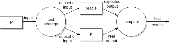
The most crucial step in this process is the selection of the subset of the input domain which will serve as the test set. This test set must be adequate with respect to some chosen test criterion. In Section 13.1.1, we elaborate upon the notion of test adequacy.
Test techniques generally use some systematic means of deriving test cases. These test cases are meant to provoke failures. Thus, the main objective is fault detection. Alternatively, our test objective could be to increase our confidence in failure-free behavior. These quite different test objectives, and their impact on the test selection problem, are the topic of Section 13.1.2.
To test whether the objectives are reached, test cases are tried in order that faults manifest themselves. A quite different approach is to view testing as fault prevention. This leads us to another dimension of test objectives, which to a large extent parallels the evolution of testing strategies over the years. This evolution is discussed in Section 13.1.3.
Finally, the picture so far considers each fault equally hazardous. In reality, there are different types of fault, and some faults are more harmful than others. All techniques to be discussed in this chapter can easily be generalized to cover multiple classes of faults, each with its own acceptance criteria.
Some faults are critical and we will have to exert ourselves in order to find those critical faults. Special techniques, such as fault-tree analysis, have been developed to this end. Using fault-tree analysis, we try to derive a contradiction by reasoning backwards from a given, undesirable, end situation. If such a contradiction can be derived, we have shown that that particular situation can never be reached.
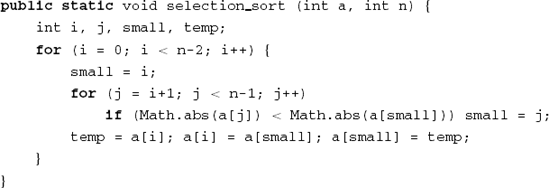
Consider the program text in Figure 13.3 and a test set S containing just one test case:
n = 2, A[0] = 10, A[1] = 5
If we execute the program using S, then all statements are executed at least once. If our criterion to judge the adequacy of a test set is that 100% of the statements are executed, then S is adequate. If our criterion is that 100% of the branches are executed, then S is not adequate, since the (empty) else branch of the if statement is not executed by S.
A test adequacy criterion thus specifies requirements for testing. It can be used in different ways: as stopping rule, as measurement, or as test case generator. If a test adequacy criterion is used as a stopping rule, it tells us when sufficient testing has been done. If statement coverage is the criterion, we may stop testing if all statements have been executed by the tests done so far. In this view, a test set is either good or bad; the criterion is either met, or it isn't. If we relax this requirement a bit and use, say, the percentage of statements executed as a test quality criterion, then the test adequacy criterion is used as a measurement. Formally, it is a mapping from the test set to the interval [0, 1]. Note that the stopping-rule view is in fact a special case of the measurement view. Finally, the test adequacy criterion can be used in the test selection process. If 100% statement coverage has not been achieved yet, an additional test case is selected that covers one or more untested statements. This generative view is used in many test tools.
Test adequacy criteria are closely linked to test techniques. For example, coverage-based test techniques keep track of which statements, branches, and so on, are executed, and this gives us an easy handle to determine whether a coverage-based adequacy criterion has been met or not. The same test technique, however, does not help us in assessing whether all error-prone points in a program have been tested. In a sense, a given test adequacy criterion and the corresponding test technique are opposite sides of the same coin.
Suppose we wish to test some component P which sorts an array A[0 .. n-1] of integers, 1 ≤ n ≤1 000. Since exhaustive testing is not feasible, we are looking for a strategy in which only a small number of tests are exercised. One possible set of test cases is the following:
Let n assume values 0, 1, 17 and 1 000. For each of n = 17 and n = 1 000, choose three values for the array A:
Aconsists of randomly selected integers;Ais sorted in ascending order;Ais sorted in descending order.
In following this type of constructive approach, the input domain is partitioned into a finite, small number of subdomains. The underlying assumption is that these subdomains are equivalence classes, i.e. from a testing point of view each member from a given subdomain is as good as any other. For example, we have tacitly assumed that one random array of length 17 is as good a test as any other random array of length i with 1 < i < 1000.
Suppose the actual sorting algorithm used is the one from Figure 13.3. If the tests use positive integers only, the output will be correct. The output will not be correct if a test input happens to contain negative integers.
The test set using positive integers only does not reveal the fault because the inputs in the subdomains are not really interchangeable (instead of comparing the values of array entries, the algorithm compares their absolute values). Any form of testing which partitions the input domain works perfectly if the right subdomains are chosen. In practice however, we generally do not know where the needles are hidden, and the partition of the input domain is likely to be imperfect.
Both functional and structural testing schemes use a systematic means to determine subdomains. They often use peculiar inputs to test peculiar cases. Their intention is to provoke failure behavior. Their success hinges on the assumption that we can indeed identify subdomains with a high failure probability. Though this is a good strategy for fault detection, it does not necessarily inspire confidence.
The user of a system is interested in the probability of failure-free behavior. Following this line of thought, we are not so much interested in the faults themselves, but rather in their manifestations. A fault which frequently manifests itself will, in general, cause more damage than a fault which seldom shows up. This is precisely what we hinted at above when we discussed fault detection and confidence building as possible test objectives.
If failures are more important than faults, the goal pursued during the test phase may also change. In that case, we will not pursue the discovery of as many faults as possible but will strive for high reliability. Random testing does not work all that well if we want to find as many faults as possible — hence the development of different test techniques. When pursuing high reliability, however, it is possible to use random input.
In order to obtain confidence in the daily operation of a software system, we have to mimic that situation. This requires the execution of a large number of test cases that represent typical usage scenarios. Random testing does at least as good a job in this respect as any form of testing based on partitioning the input domain.
This approach has been applied in the Cleanroom development method. In this method, the development of individual components is done by programmers who are not allowed to actually execute their code. The programmer must then convince himself of the correctness of his components using manual techniques such as stepwise abstraction (see also Section 13.4).
In the next step, these components are integrated and tested by someone else. The input for this process is generated according to a distribution which follows the expected operational use of the system. During this integration phase, one tries to reach a certain required reliability level. Experiences with this approach are positive.
The quantitative assessment of failure probability brings us into the area of software reliability. Section 13.10 is devoted to this topic.
In the early days of computing, programs were written and then debugged to make sure that they ran properly. Testing and debugging were largely synonymous terms. Both referred to an activity near the end of the development process when the software had been written, but still needed to be 'checked out'.
Today's situation is rather different. Testing activities occur in every phase of the development process. They are carefully planned and documented. The execution of software to compare actual behavior with expected behavior is only one aspect out of many.
Gelperin and Hetzel (1988) identify four major testing models. These roughly parallel the historical development of test practices. The models and their primary goals are given in Table 13.1.
Table 13.1. Major testing models (Source: D. Gelperin and B. Hetzel, The growth of software testing, Communications of the ACM 31(6), pp. 687–95, © 1988. Reproduced by permission of the Association for Computing Machinery, Inc.)
Model | Primary goal |
|---|---|
Phase models | |
Demonstration | Make sure that the software satisfies its specification |
Destruction | Detect implementation faults |
Life cycle models | |
Evaluation | Detect requirements, design, and implementation faults |
Prevention | Prevent requirements, design, and implementation faults |
The primary goal of the demonstration model is to make sure that the program runs and solves the problem. The strategy is like that of a constructive mathematical proof. If the software passes all tests from the test set, it is claimed to satisfy the requirements. The strategy gives no guidelines as to how to obtain such a test set. A poorly chosen test set may mask poor software quality. Most programmers will be familiar with the process of testing their own programs by carefully reading them or executing them with selected input data. If this is done very carefully, it can be beneficial. This method also holds some dangers, however. We may be inclined to consider this form of testing as a method to convince ourselves or someone else that the software does not contain errors. We will then, partly unconsciously, look for test cases which support this hypothesis. This type of demonstration-oriented approach to testing is not to be advocated.
Proper testing is a very destructive process. A program should be tested with the purpose of finding as many faults as possible. A test can only be considered successful if it leads to the discovery of at least one fault. (In a similar way, a visit to your physician is only successful if he finds a 'fault' and we generally consider such a visit unsatisfactory if we are sent home with the message that nothing wrong could be found.) In order to improve the chances of producing a high quality system, we should reverse the strategy and start looking for test cases that do reveal faults. This may be termed a proof by contradiction. The test set is then judged by its ability to detect faults.
Since we do not know whether any residual faults are left, it is difficult to decide when to stop testing in either of these models. In the demonstration-oriented model, the criteria most often used to determine this point in time seem to be the following:
stop if the test budget has run out;
stop if all test cases have been executed without any failures occurring.
The first criterion is pointless, since it does not tell us anything about the quality of the test effort. If there is no money at all, this criterion is most easily satisfied. The second criterion is pointless as well, since it does not tell us anything about the quality of the test cases.
The destruction-oriented model usually entails some systematic way of deriving test cases. We may then base our stop criterion on the test adequacy criterion that corresponds to the test technique used. An example of this might be: 'We stop testing if 100% of the branches are covered by the set of test cases and all test cases yield an unsuccessful result'.
Both these models view testing as one phase in the software development process. As noted before, this is not a very good strategy. The life-cycle-testing models extend testing activities to earlier phases. In the evaluation-oriented model, the emphasis is on analysis and review techniques to detect faults in requirements and design documents. In the prevention model, emphasis is on the careful planning and design of test activities. For example, the early design of test cases may reveal that certain requirements cannot be tested and thus such an activity helps to prevent errors from being made in the first place. Test-driven development falls into this category as well.
We may observe a gradual shift of emphasis in test practice, from a demonstration-like approach to prevention-oriented methods. Though many organizations still concentrate their test effort late in the development life cycle, various organizations have shown that upstream testing activities can be most effective. Quantitative evidence of this is provided in Section 13.8.3.
Testing need not only result in software with fewer errors. Testing also results in valuable knowledge (error-prone constructs and so on) which can be fed back into the development process. In this view, testing is a learning process, which can be given its proper place in an improvement process.
In the following subsections we discuss the various verification and validation activities which can be performed during the requirements engineering, design, implementation, and maintenance phases. In doing so, we also indicate the techniques and tools that may be applied. These techniques and tools are further discussed in subsequent sections. A summary is given in Table 13.2.
Table 13.2. Activities in the various phases of the software life cycle (Adapted from: W.R. Adrion, M.A. Branstad, and J.C. Cherniavski, Validation, verification, and testing of computer software, ACM Computing Surveys 14(2), © 1982. Reproduced by permission of the Association for Computing Machinery, Inc.)
Phase | Activities |
|---|---|
Requirements engineering | — determine test strategy — test requirements specification — generate functional test data |
Design | — check consistency between design and requirements specification — evaluate the software architecture — test the design — generate structural and functional test data |
Implementation | — check consistency between design and implementation — test implementation — generate structural and functional test data — execute tests |
Maintenance | — repeat the above tests in accordance with the degree of redevelopment |
Software developers aim for clean code that works. We try to accomplish that by first focusing on the 'clean code' part, and next on the 'that works' part. The clean code part is about proper analysis and design, writing elegant and robust code, and so on. Only after we're done with that, do we start testing to make sure the software works properly. Test-driven development (TDD) takes the opposite approach: we first make sure the software works and then tackle the clean code part. We discuss test-driven development in Section 13.2.5.
The verification and validation techniques applied during this phase are strongly dependent upon the way in which the requirements specification has been laid down. Something which should be done at the very least is to conduct a careful review or inspection in order to check whether all aspects of the system have been properly described. As we saw earlier, errors made at this stage are very costly to repair if they go unnoticed until late in the development process. (Boehm, 1984b) gives four essential criteria for a requirements specification:
completeness;
consistency;
feasibility;
testability.
Testing a requirements specification should primarily be aimed at testing these criteria.
The aim of testing the completeness criterion is to determine whether all components are present and described completely. A requirements specification is incomplete if it contains such phrases as 'to be determined' or if it contains references to undefined elements. We should also watch for the omission of functions or products, such as back-up or restart procedures and test tools to be delivered to the customer.
A requirements specification is consistent if its components do not contradict each other and the specification does not conflict with external specifications. We thus need both internal and external consistency. Moreover, each element in the requirements specification must be traceable. It must, for instance, be possible to decide whether a natural language interface is really needed.
According to Boehm, feasibility has to do with more than functional and performance requirements. The benefits of a computerized system should outweigh the associated costs. This must be established at an early stage and necessitates timely attention to user requirements, maintainability, reliability, and so on. In some cases, the project's success is very sensitive to certain key factors, such as safety, speed, availability of certain types of personnel; these risks must be analyzed at an early stage.
Lastly, a requirements specification must be testable. In the end, we must be able to decide whether or not a system fulfills its requirements. So requirements must be specific, unambiguous, and quantitative. The quality-attribute scenario framework from (Bass et al., 2003) is an example of how to specify such requirements; see also Section 6.3.
Many of these points are raised by (Poston, 1987). According to Poston, the most likely errors in a requirements specification can be grouped into the following categories:
missing information (about functions, interfaces, performance, constraints, reliability, and so on);
wrong information (not traceable, not testable, ambiguous, and so forth);
extra information (bells and whistles).
Using a standard format for documenting the requirements specification, such as IEEE Standard 830 (discussed in Chapter 9), may help enormously in preventing these types of errors occurring in the first place.
Useful techniques for testing the degree to which criteria have been met are mostly manual (reading documents, inspections, reviews). Scenarios for the expected use of the system can be devised with the prospective users of the system. If requirements are already expressed in use cases, such scenarios are readily available. In this way, a set of functional tests is generated.
At this stage also, a general test strategy for subsequent phases must be formulated. It should encompass the choice of particular test techniques; evaluation criteria; a test plan; a test scheme; and test documentation requirements. A test team may also be formed at this stage. These planning activities are dealt with in Section 13.3.
The criteria mentioned previously (completeness, consistency, feasibility, and testability) are also essential for the design. The most likely errors in design resemble the kind of errors one is inclined to make in a requirements specification: missing, wrong, and extraneous information. For the design too, a precise documentation standard is of great help in preventing these types of errors. IEEE Standards 1471 and 1016, discussed in Chapters 11 and 12, respectively, are examples of such standards.
During the architectural design phase, a high-level conceptual model of the system is developed in terms of components and their interaction. This architecture can be assessed, for example by generating scenarios which express quality concerns, such as maintainability and flexibility, in very concrete terms and evaluating how the architecture handles these scenarios; see also Section 11.5.
During the design phase, we decompose the total system into subsystems and components, starting from the requirements specification. We may then develop tests based on this decomposition process. Design is not a one-shot process. During the design process a number of successive refinements will be made, resulting in layers showing increasing detail. Following this design process, more detailed tests can be developed as the lower layers of the design are decided upon.
We may also test the design itself. This includes tracing elements from the requirements specification to the corresponding elements in the design description, and vice versa. Well-known techniques for doing so are, amongst others, simulation, design walkthroughs, and design inspections.
In the requirements engineering phase, the possibilities for formally documenting the resulting specification are limited. Most requirements specifications make excessive use of natural language descriptions. For the design phase, there are ample opportunities to formally document the resulting specification. The more formally the design is specified, the more possibilities we have for applying verification techniques, as well as formal checks for consistency and completeness.
During the implementation phase, we do the 'real' testing. One of the most effective techniques to find errors in a program text is to carefully read that text, or have it read. This technique has been successfully applied for a long time. Somewhat formalized variants are known as 'code inspection' and 'code walkthrough'. We may also apply the technique of stepwise abstraction: the function of the code is determined in a number of abstraction steps, starting from the code itself. We may try to prove the correctness of the code using formal verification techniques. The various manual test techniques are discussed in Section 13.4.
There are many tools to support the testing of code. We may distinguish between tools for static analysis and tools for dynamic analysis. Static analysis tools inspect the program code without executing it. They include tests such as: are all variables declared and given a value before they are used? Dynamic analysis tools are used in conjunction with the actual execution of the code, for example tools that keep track of which portions of the code have been covered by the tests so far.
All of the above techniques are aimed at evaluating the quality of the source code as well as its compliance with design specifications and code documentation.
It is crucial to control the test information properly while testing the code. Tools may help us to do so, for example, test drivers generate the test environment for a component to be tested, test stubs simulate the function of a component not yet available, and test data generators provide us with data. In bottom-up testing, we will, in general, make much use of test drivers, while top-down testing implies the use of test stubs. The test strategy (top-down versus bottom-up) may be partly influenced by the design technique used. If the high level, architectural design is implemented as a skeletal system whose holes yet have to be filled in, that skeletal system can be used as a test driver.
Tools (test harnesses and test systems) may also be profitable while executing the tests. A simple and yet effective tool is one which compares test results with expected results. The eye is a very unreliable medium. After a short time, all results look OK. An additional advantage of this type of tool support is that it helps to achieve a standard test format. This, in turn, helps with regression testing.
On average, more than 50% of total life-cycle costs is spent on maintenance. If we modify the software after a system has become operational (because an error is found late on, or because the system must be adapted to changed requirements), we will have to test the system anew. This is called regression testing. To have this proceed smoothly, the quality of the documentation and the possibilities for tool support, are crucial factors.
In a retest-all approach, all tests are rerun. Since this may consume a lot of time and effort, we may also opt for a selective retest, in which only some of the tests are rerun. A regression test selection technique is then used to decide which subset should be rerun. We would like this technique to include all tests in which the modified and the original program produce different results, while omitting tests that produce the same results.
Suppose our library system needs to be able to prevent borrowing of items by members that are on a black list. We could start by redesigning part of the system and implementing the necessary changes: a new table, BlackList, and appropriate checks in method Borrow. We also have to decide when members are put on the black list, and how to get them off that list. After having done all the necessary analysis and design, and implemented the changes accordingly, we devise test cases to test for the new functionality.
This order of events is completely reversed in test-driven development (TDD). In test-driven development, we first write a few tests for the new functionality. We may start very simple, and add a test in the start-up method to ensure that the black list is initially empty:
assertEquals(0, BlackList)
Of course, this test will fail. To make it succeed, we have to introduce BlackList, and set it equal to 0. At the same time, we make a list of things still to be done, such as devising a proper type for BlackList, including operations to add and remove members to that list, an update of Borrow to check whether a person borrowing an item is on the black list, and so on. This list of things to be done is similar to the backlog used by architects while architecting a system (see Section 11.2).
After we have made the simple test work, the new version of the system is inspected to see whether it can be improved. Another small change is contemplated. We may for example decide to make BlackList into a proper list, and write some simple tests to see that after adding an item to the list, that item is indeed in the list. Again, the test will fail and we update the system accordingly. Possibly, improvements can be made now since the library system probably contains other list-type classes that we can inherit from and some duplicate code can be removed. And so on.
Test-driven development is one of the practices of eXtreme Programming (see Section 3.2.4). As such, it is part of the agile approach to system development which favors small increments and redesign (refactoring) where needed rather than big design efforts. The practice is usually supported by an automated unit testing framework, such as JUnit for Java, that keeps track of the test set and reports back readable error messages for tests that fail (Hunt and Thomas, 2003). The assertEquals method used above is one of the methods provided by the JUnit framework. The framework allows for a smooth integration of coding and unit testing. On the fly, a test set is built that forms a reusable asset during the further evolution of the system. JUnit and similar frameworks have greatly contributed to the success of test-driven development.
The way of working in each iteration of test-driven development consists of the following steps:
Add a test.
Run all tests and observe that the one added fails.
Make a small change to the system to make the test work.
Run all tests again and observe that they run properly.
Refactor the system to remove duplicate code and improve its design.
In pure eXtreme Programming, iterations are very small, and may take from a few minutes up to, say, an hour. But test-driven development can also be done in bigger leaps and can be combined with more traditional approaches.
Test-driven development is much more than a test method. It is a different way of developing software. The effort put into the upfront development of test cases forces one to think more carefully of what it means for the current iteration to succeed or fail. Writing down explicit test cases subsumes part of the analysis and design work. Rather than producing UML diagrams during requirements analysis, we produce tests. And these tests are used immediately, by the same person that implemented the functionality that the test exercises. Testing then is not an afterthought, but becomes an integral part of the development process. Another benefit is that we have a test set and a test criterion to decide on the success of the iteration. Experiments with test-driven development indicate that it increases productivity and reduces defect rates.
Like the other phases and activities of the software development process, the testing activities need to be carefully planned and documented. Since test activities start early in the development life cycle and span all subsequent phases, timely attention to the planning of these activities is of paramount importance. A precise description of the various activities, responsibilities and procedures must be drawn up at an early stage.
The planning of test activities is described in a document called the software verification and validation plan. We base our discussion of its contents on IEEE Standard 1012. (IEEE1012, 2004) describes verification and validation activities for a waterfall-like life cycle in which the following phases are identified:
concept phase
requirements phase
design phase
implementation phase
test phase
installation and checkout phase
operation and maintenance phase
The first of these, the concept phase, is not discussed in the present text. Its aim is to describe and evaluate user needs. It produces documentation which contains, for example, a statement of user needs, results of feasibility studies, and policies relevant to the project. The verification and validation plan is also prepared during this phase. In our approach, these activities are included in the requirements engineering phase.
The sections to be included in the verification and validation (V&V) plan are listed in Table 13.3. The structure of this plan resembles that of other standards discussed earlier. The plan starts with an overview and gives detailed information on every aspect of the topic being covered.
More detailed information on the many V&V tasks covered by this plan can be found in (IEEE1012, 2004). Following the organization proposed in this standard, the bulk of the test documentation can be structured along the lines identified in Table 13.4. The Test Plan is a document describing the scope, approach, resources, and schedule of intended test activities. It can be viewed as a further refinement of the verification and validation plan and describes in detail the test items, features to be tested, testing tasks, who will do each task, and any risks that require contingency planning.
The Test Design Specification defines, for each software feature or combination of such features, the details of the test approach and identifies the associated tests. The Test Case Specification defines inputs, predicted outputs, and execution conditions for each test item. The Test Procedure Specification defines the sequence of actions for the execution of each test. Together with the Test Plan, these documents describe the input to the test execution.
The Test Item Transmittal Report specifies which items are going to be tested. It lists the items, specifies where to find them, and gives the status of each item. It constitutes the release information for a given test execution.
The final three reports are the output of the test execution. The Test Log gives a chronological record of events. The Test Incident Report documents all events observed that require further investigation. In particular, this includes tests from which the outputs were not as expected. Finally, the Test Summary Report gives an overview and evaluation of the findings. A detailed description of the contents of these various documents is given in (IEEE829, 1998).
Table 13.3. Sample contents of the Verification and Validation Plan (Source: IEEE Standard for Software Verification and Validation Plans, IEEE Standard 1012 ©2004. Reproduced by permission of IEEE.)
|
A lot of research effort is spent on finding techniques and tools to support testing. Yet, a plethora of heuristic test techniques have been applied since the beginning of the programming era. These heuristic techniques, such as walkthroughs and inspections, often work quite well, although it is not always clear why.
Test techniques can be separated into static and dynamic analysis techniques. During dynamic analysis, the program is executed. With this form of testing, the program is given some input and the results of the execution are compared with the expected results. During static analysis, the software is generally not executed. Many static test techniques can also be applied to non-executable artifacts such as a design document or user manual. It should be noted, though, that the borderline between static and dynamic analysis is not very sharp.
A large part of the static analysis is nowadays done by the language compiler. The compiler checks whether all variables have been declared, whether each method call has the proper number of actual parameters, and so on. These constraints are part of the language definition. We may also apply a more strict analysis of the program text, such as a check for initialization of variables, or a check on the use of non-standard, or error-prone, language constructs. In a number of cases, the call to a compiler is parameterized to indicate the checks one wants to be performed. Sometimes, separate tools are provided for these checks.
The techniques to be discussed in the following subsections are best classified as static techniques. The techniques for coverage-based, fault-based, and error-based testing, to be discussed in Sections 13.5 to 13.7, are mostly dynamic in nature.
We all read, and reread, and reread our program texts. It is the most traditional test technique we know of. It is also a very successful technique for finding faults in a program text (or a specification or a design).
In general, it is better to have someone else read your texts. The author of a text knows all too well what the program (or any other type of document) ought to convey. For this reason, the author may be inclined to overlook things, suffering from some sort of trade blindness.
A second reason why reading by the author himself might be less fruitful, is that it is difficult to adopt a destructive attitude towards one's own work. Yet such an attitude is needed for successful testing.
A somewhat institutionalized form of reading each other's programs is known as peer review. This is a technique for anonymously assessing programs for quality, readability, usability, and so on.
Each person partaking in a peer review is asked to hand in two programs: a 'best' program and one of lesser quality. These programs are then randomly distributed amongst the participants. Each participant assesses four programs: two 'best' programs and two programs of lesser quality. After all the results have been collected, each participant gets the (anonymous) evaluations of their programs, as well as the statistics of the whole test.
The primary goal of this test is to give the programmer insight into his own capabilities. The practice of peer reviews shows that programmers are quite capable of assessing the quality of their peers' software.
A necessary precondition for successfully reading someone else's code is a business-like attitude. Weinberg (1971) coined the term egoless programming for this. Many programmers view their code as something personal, like a diary. Derogatory remarks ('how could you be so stupid as to forget that initialization') can disastrously impair the effectiveness of such assessments. The opportunity for such an antisocial attitude to occur seems to be somewhat smaller with the more formalized manual techniques.
Walkthroughs and inspections are both manual techniques that spring from the traditional desk-checking of program code. In both cases, it concerns teamwork and the product to be inspected is evaluated in a formal session, following precise procedures.
Inspections are sometimes called Fagan inspections, after their originator (Fagan, 1976, 1986). In an inspection, the code to be assessed is gone through, statement by statement. The members of the inspection team (usually four people) get the code, its specification, and the associated documents a few days before the session takes place.
Each member of the inspection team has a well-defined role. The moderator is responsible for the organization of inspection meetings. He chairs the meeting and ascertains that follow-up actions agreed upon during the meeting are indeed performed. The moderator must ensure that the meeting is conducted in a businesslike, constructive way and that the participants follow the correct procedures and act as a team. The team usually has two inspectors or readers, knowledgeable peers that paraphrase the code. Finally, the code author is a largely silent observer. He knows the code to be inspected all too well and is easily inclined to express what he intended rather than what is actually written down. He may, though, be consulted by the inspectors.
During the formal session, the inspectors paraphrase the code, usually a few lines at a time. They express the meaning of the text at a higher level of abstraction than what is actually written down. This gives rise to questions and discussions which may lead to the discovery of faults. At the same time, the code is analyzed using a checklist of faults that often occur. Examples of possible entries in this checklist are:
wrongful use of data: variables not initialized, array index out of bounds, dangling pointers;
faults in declarations: the use of undeclared variables or the declaration of the same name in nested blocks;
faults in computations: division by zero, overflow (possible in intermediate results too), wrong use of variables of different types in the same expression, faults caused by an erroneous understanding of operator priorities;
faults in relational expressions: using an incorrect operator (> instead of ≥, = instead of ==) or an erroneous understanding of priorities of Boolean operators;
faults in control flow: infinite loops or a loop that is executed n + 1 or n − 1 times rather than n times;
faults in interfaces: an incorrect number of parameters, parameters of the wrong type, or an inconsistent use of global variables.
The result of the session is a list of problems identified.
These problems are not resolved during the formal session itself. This might easily lead to quick fixes and distract the team from its primary goal. After the meeting, the code author resolves all the issues raised and the revised code is verified once again. Depending on the number of problems identified and their severity, this second inspection may be done by the moderator only or by the complete inspection team.
Since the goal of an inspection is to identify as many problems as possible in order to improve the quality of the software to be developed, it is important to maintain a constructive attitude towards the developer whose code is being assessed.[23] The results of an inspection therefore are often marked confidential. These results should certainly not play a role in the formal assessment of the developer in question.
In a walkthrough, the team is guided through the code using test data. The test data is mostly of a fairly simple kind, otherwise tracing the program logic soon becomes too complicated. The test data serves as a way of starting a discussion, rather than as a serious test of the program. In each step of this process, the developer may be questioned regarding the rationale of the decisions. In many cases, a walkthrough boils down to some sort of manual simulation.
Both walkthroughs and inspections may profitably be applied at all stages of the software life cycle. The only precondition is that there is a clear, testable document. It is estimated that these review methods detect 50–90% of defects (Boehm and Basili, 2001). Both techniques serve not only to find faults: if properly applied, these techniques may help to promote team spirit and morale. At the technical level, the people involved may learn from each other and enrich their knowledge of algorithms, programming style, programming techniques, error-prone constructions, and so on. Thus, these techniques also serve as a vehicle for process improvement. Under the general umbrella of 'peer reviews', they are part of the CMM level 3 key process area Verification (see Section 6.6).
A potential danger of this type of review is that it remains too shallow. The people involved may become overwhelmed with information; they may have insufficient knowledge of the problem domain; their responsibilities may not have been clearly delineated. As a result, the review process does not pay off sufficiently.
Parnas and Weiss (1987) describe a type of review process in which the people involved have to play a more active role. They distinguish between different types of specialized design review. Each of these reviews concentrates on certain desirable properties of the design. As a consequence, the responsibilities of the people involved are clear. The reviewers have to answer a list of questions ('under which conditions may this function be called?', 'what is the effect of this function on the behavior of other functions?', and so on). In this way, the reviewers are forced to study carefully the design information received. Problems with the questionnaire and documentation can be posed to the developers, and the completed questionnaires are discussed by the developers and reviewers. Experiments suggest that inspections with specialized review roles are more effective than inspections in which review roles are not specialized.
A very important component of Fagan inspections is the meeting in which the document is discussed. Since meetings may incur considerable costs or time-lags, one may try to do without them. Experiments suggest that the added value of group meetings, in terms of the number of problems identified, is quite small.
The most complete static analysis technique is the proof of correctness. In a proof of correctness we try to prove that a program meets its specification. In order to be able to do so, the specification must be expressed formally. We mostly do this by expressing the specification in terms of two assertions which hold before and after the program's execution, respectively. Next, we prove that the program transforms one assertion (the precondition) into the other (the postcondition). This is generally denoted as:
{P} S {Q}Here, S is the program, P is the precondition, and Q is the postcondition. Termination of the program is usually proved separately. The above notation should thus be read as: if P holds before the execution of S and S terminates, then Q holds after the execution of S.
Formally verifying the correctness of a not-too-trivial program is a very complex affair. Some sort of tool support is helpful, therefore. Tools in this area are often based on heuristics and proceed interactively.
Correctness proofs are very formal and, for that reason, they are often difficult for the average programmer to construct. The value of formal correctness proofs is sometimes disputed. We may state that the thrust in software is more important than some formal correctness criterion. Also, we cannot formally prove every desirable property of software. Whether we built the right system can only be decided upon through testing (validation).
On the other hand, it seems justified to state that a thorough knowledge of this type of formal technique will result in better software.
In the top-down development of software components, we often employ stepwise refinement. At a certain level of abstraction, the function to be executed will be denoted by a description of that function. At the next level, this description is decomposed into more basic units.
Stepwise abstraction is just the opposite. Starting from the instructions of the source code, the function of the component is built up in a number of steps. The function thus derived should comply with the function as described in the design or requirements specification.
To illustrate this technique, consider the search routine of Figure 13.4. We know, from the accompanying documentation for instance, that the elements in array a (from index 1 up to index a.length) are sorted when this routine is called.
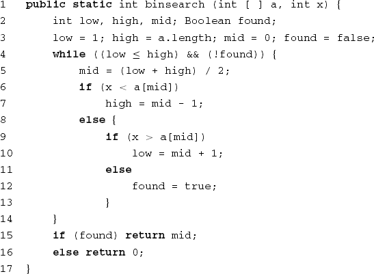
We start the stepwise abstraction with the instructions of the if statement on lines 6–13. x is compared with a[mid]. Depending on the result of this comparison, one of high, low, and found is given a new value. If we take into account the assignments on lines 3 and 5, the function of this if statement can be summarized as
stop searching (found =true) if x == a[mid], or shorten the interval [low .. high] that might contain x, to an interval [low' .. high'], where high' — low'<high - low
Alternatively, this may be described as a postcondition to the if statement:
(found ==true andx == a[mid])or(found ==false andx∉a[1 .. low' - 1]andx∉a[high' + 1 .. a.length]andhigh' - low'<high - low)
Next, we consider the loop in lines 4–14, together with the initialization on line 3. As regards termination of the loop, we may observe the following. If 1 ≤ a.length upon calling the routine, then low ≤ high at the first execution of lines 4–14. From this, it follows that low ≤ mid ≤ high. If the element searched for is found, the loop stops and the position of that element is returned. Otherwise, either high is assigned a smaller value, or low is assigned a higher value. Thus, the interval [low .. high] gets smaller. At some point in time, the interval will have length of 1, i.e. low = high (assuming the element still is not found). Then, mid will be assigned that same value. If x still does not occur at position mid, either high will be assigned the value low − 1, or low will be assigned the value high + 1. In both cases, low > high and the loop terminates. Together with the postcondition given earlier, it then follows that x does not occur in the array a. The function of the complete routine can then be described as:
result = 0 x ∉ a[1 .. a.length]
1 ≤ result ≤ a.length x = a[result]So, stepwise abstraction is a bottom-up process to deduce the function of a piece of program text from that text.
In coverage-based test techniques, the adequacy of testing is expressed in terms of the coverage of the product to be tested, for example, the percentage of statements executed or the percentage of functional requirements tested.
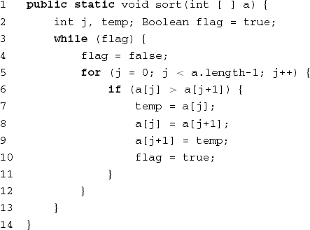
Coverage-based testing is often based on the number of instructions, branches or paths visited during the execution of a program. It is helpful to base the discussion of this type of coverage-based testing on the notion of a control graph. In this control graph, nodes denote actions, while the (directed) edges connect actions with subsequent actions (in time). A path is a sequence of nodes connected by edges. The graph may contain cycles, i.e. paths p1, ..., pn such that p1 = pn. These cycles correspond to loops in the program (or gotos). A cycle is 'simple' if its inner nodes are distinct and do not include p1 (or pn, for that matter). Note that a sequence of actions (statements) that has the property that whenever the first action is executed, the other actions are executed in the given order may be collapsed into a single, compound, action. So when we draw the control graph for the program in Figure 13.5, we may put the statements on lines 7–10 in different nodes, but we may also put them all in a single node.
In Sections 13.5.1 and 13.5.2 we discuss a number of test techniques which are based on coverage of the control graph of the program. Section 13.5.3 illustrates how these coverage-based techniques can be applied at the requirements specification level.
During the execution of a program, we follow a certain path through its control graph. If some node has multiple outgoing edges, we choose one of those (which is also called a branch). In the ideal case, the tests collectively traverse all possible paths. This all-paths coverage is equivalent to exhaustively testing the program.
In general, this is not possible. A loop often results in an infinite number of possible paths. If we do not have loops, but only branch instructions, the number of possible paths increases exponentially with the number of branching points. There may also be paths that are never executed (quite likely, the program contains a fault in that case). We therefore search for a criterion which expresses the degree to which the test data approximates the ideal coverage.
Many such criteria can be devised. The most obvious is the criterion which counts the number of statements (nodes in the graph) executed. It is called the all-nodes coverage, or statement coverage. This criterion is rather weak because it is relatively simple to construct examples in which 100% statement coverage is achieved, while the program is nevertheless incorrect.
Consider as an example the program given in Figure 13.5. It is easy to see that a single test, with n = 2, a[1] = 5, a[2] = 3, results in each statement being executed at least once. So, this one test achieves 100% statement coverage. However, if we change, for example, the test a[i] ≥ a[i - 1] in line 6 to a[i] = a[i - 1], we still obtain a 100% statement coverage with this test. Although this test also yields the correct answer, the changed program is incorrect.
We get a stronger criterion if we require that, at each branching node in the control graph, all possible branches are chosen at least once. This is known as all-edges coverage or branch coverage. Here too, 100% coverage is no guarantee of program correctness.
Nodes that contain a condition, such as the Boolean expression in an if statement, can be a combination of elementary predicates connected by logical operators. A condition of the form
i>0orj>0
requires at least two tests to guarantee that both branches are taken. For example,
i = 1, j = 1
and
i = 0, j = 1
will do. Other possible combinations of truth values of the atomic predicates (i= 1, j= 0 and i= 0, j = 0) need not be considered to achieve branch coverage. Multiple condition coverage requires that all possible combinations of elementary predicates in conditions be covered by the test set. This criterion is also known as extended branch coverage.
Finally, McCabe's cyclomatic complexity metric (McCabe, 1976) has also been applied to testing. This criterion is also based on the control graph representation of a program. A basis set is a maximal linearly independent set of paths through a graph. The cyclomatic complexity (CV) equals this number of linearly independent paths (see also Section 12.1.4). Its formula is
Here, V(G) is the graph's cyclomatic number:
where
e = the number of edges in the graph
n = the number of nodes
p = the number of maximal connected subgraphs, i.e. subgraphs for which each pair of nodes is connected by some path
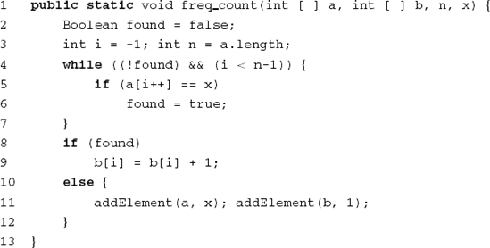
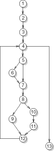
As an example, consider the program text of Figure 13.6. The corresponding control graph is given in Figure 13.7. For this graph, e = 15, n = 13, and p = 1. So V(G) = 3 and CV(G) = 4. A possible set of linearly independent paths for this graph is: {1-2-3-4-5-6-7-8-9-12-4, 5–7, 8-10-11, 4–13}.
A possible test strategy is to construct a test set such that all linearly independent paths are covered. This adequacy criterion is known as the cyclomatic-number criterion.
Starting from the control graph of a program, we may also consider how variables are treated along the various paths. This is termed data flow analysis. With data flow analysis too, we may define test adequacy criteria and use these criteria to guide testing.
In data flow analysis, we consider the definitions and uses of variables along execution paths. A variable is defined in a certain statement if it is assigned a (new) value because of the execution of that statement. After that, the new value is used in subsequent statements. A definition in statement X is alive in statement Y if there exists a path from X to Y in which that variable is not assigned a new value at some intermediate node. In the example in Figure 13.5, for instance, the definition of flag at line 4 is still alive at line 9 but not at line 10. A path such as the one from line 4 to 9 is called definition-clear (with respect to flag). Algorithms to determine such facts are commonly used in compilers in order to allocate variables optimally to machine registers.
We distinguish between two types of variable use: P-uses and C-uses. P-uses are predicate uses, such as those in the conditional part of an if statement. All other uses are C-uses. Examples of the latter are uses in computations or I/O statements.
A possible test strategy is to construct tests which traverse a definition-clear path between each definition of a variable to each (P- or C-) use of that definition and each successor of that use. (We have to include each successor of a use to force all branches following a P-use to be taken.) We are then sure that each possible use of a definition is being tested. This strategy is known as all-uses coverage. A slightly stronger criterion requires that each definition-clear path is either cycle-free or a simple cycle. This is known as all-DU-paths coverage. Several weaker data flow criteria can be defined as well:
All-defs coverage simply requires the test set to be such that each definition is used at least once.
All-C-uses/Some-P-uses coverage requires definition-clear paths from each defi-nition to each computational use. If a definition is used only in predicates, at least one definition-clear path to a predicate use must be exercised.
All-P-uses/Some-C-uses coverage requires definition-clear paths from each defini-tion to each predicate use. If a definition is used only in computations, at least one definition-clear path to a computational use must be exercised.
All-P-uses coverage requires definition-clear paths from each definition to each predicate use.
Program code can be easily transformed into a graph model, thus allowing for all kinds of test adequacy criteria based on graphs. Requirements specifications, however, may also be transformed into a graph model. As a consequence, the various coverage-based adequacy criteria can be used in both black-box and white-box testing techniques.
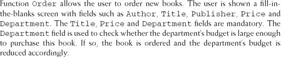
Consider the example fragment of a requirements specification document for our library system in Figure 13.8. We may rephrase these requirements a bit and present them in the form of elementary requirements and relations between them. The result can be depicted as a graph, where the nodes denote elementary requirements and the edges denote relations between elementary requirements; see Figure 13.9. We may use this graph model to derive test cases and apply any of the control-flow coverage criteria to assess their adequacy.
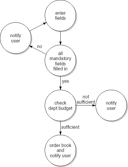
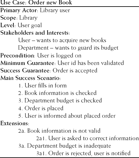
A very similar route can be followed if the requirement is expressed in the form of a use case. Figure 13.10 gives a possible rewording of the fragment from Figure 13.8. It uses the format from (Cockburn, 2001). The use case describes both the normal case, called the Main Success Scenario, as well as extensions that cover situations that branch off the normal path because of some condition. For each extension, both the condition and the steps taken are listed. Note that Figure 13.9 directly mimics the use case description from Figure 13.10. The use case description also allows us to straightforwardly derive test cases and apply control-flow coverage criteria.
Generally speaking, a major problem in determining a set of test cases is to partition the program domain into a (small) number of equivalence classes. We try to do so in such a way that testing a representative element from a class suffices for the whole class. Using control-flow coverage criteria, for example, we assume that any test of some node or branch is as good as any other such test. In the above example, for instance, we assume that any execution of the node labeled 'check dept. budget' will do.
The weak point in this procedure is the underlying assumption that the program behaves equivalently on all data from a given class. If this assumption is true, the partition is perfect and so is the test set. This assumption will not hold, in general (see also Section 13.1.2).
In coverage-based testing techniques, we consider the structure of the problem or its solution, and the assumption is that a more comprehensive covering is better. In fault-based testing strategies, we do not directly consider the artifact being tested when assessing the test adequacy. We only take into account the test set. Fault-based techniques are aimed at finding a test set with a high ability to detect faults.
We will discuss two fault-based testing techniques: error seeding and mutation testing.
Text books on statistics often contain examples along the following lines:
If we want to estimate the number of pikes in Lake Soft, we proceed as follows:
Catch a number of pikes, N, in Lake Seed;
Mark them and throw them into Lake Soft;
Catch a number of pikes, M, in Lake Soft.
Supposing that M′ out of the M pikes are found to be marked, the total number of pikes originally present in Lake Soft is then estimated as (M - M′) × N/M′.
A somewhat unsophisticated technique is to try to estimate the number of faults in a program in a similar way. The easiest way to do this is to artificially seed a number of faults in the program. When the program is tested, we discover both seeded faults and new ones. The total number of faults is then estimated from the ratio of those two numbers.
We must be aware of the fact that a number of assumptions underlie this method — amongst others, the assumption that both real and seeded faults have the same distribution.
There are various ways of determining which faults to seed in the program. A not very satisfactory technique is to construct them by hand. It is unlikely that we will be able to construct very realistic faults in this way. Faults thought up by one person have a fair chance of having been thought up already by the person that wrote the software.
Another technique is to have the program independently tested by two groups. The faults found by the first group can then be considered seeded faults for the second group. In using this technique, though, we must realize that there is a chance that both groups detect (the same type of) simple faults. As a result, the picture might well be distorted.
A useful rule of thumb for this technique is the following: if we find many seeded faults and relatively few others, the result can be trusted. The opposite is not true. This rule of thumb is more generally applicable: if, during testing of a certain component, many faults are found, it should not be taken as a positive sign. Quite the contrary, it is an indication that the component is probably of low quality. As Myers (1979) observed: 'The probability of the existence of more errors in a section of a program is proportional to the number of errors already found in that section.' The same phenomenon has been observed in some experiments, where a strong linear relationship was found between the number of defects discovered during early phases of development and the number of defects discovered later.
Suppose we have some program P which produces the correct results for some tests T1 and T2. We generate some variant P′ of P. P′ differs from P in just one place. For instance, a + is replaced by a —, or the value v1 in a loop of the form
for(var = v1; var<v2; var++)
is changed into v1 + 1 or v1 − 1. Next, P′ is tested using tests T1 and T2. Let us assume that T1 produces the same result in both cases, whereas T2 produces different results. Then T1 is the more interesting test case, since it does not discriminate between two variants of a program, one of which is certainly wrong.
In mutation testing, we generate a (large) number of variants of a program. Each of those variants, or mutants, slightly differs from the original version. Usually, mutants are obtained by mechanically applying a set of simple transformations called mutation operators (see Table 13.5).
Table 13.5. A sample of mutation operators
Replace a constant by another constant Replace a variable by another variable Replace a constant by a variable Replace an arithmetic operator by another arithmetic operator Replace a logical operator by another logical operator Insert a unary operator Delete a statement |
Next, all these mutants are executed using a given test set. As soon as a test produces a different result for one of the mutants, that mutant is said to be dead. Mutants that produce the same results for all of the tests are said to be alive. As an example, consider the erroneous sort procedure in Figure 13.3 and the correct variant thereof which compares array elements rather than their absolute values. Tests with an array which happens to contain positive numbers only will leave both variants alive. If a test set leaves us with many live mutants, then that test set is of low quality, since it is not able to discriminate between all kinds of variant of a given program.
If we assume that the number of mutants that is equivalent to the original program is 0 (normally, this number will certainly be very small), then the mutation adequacy score of a test set equals D/M, where D is the number of dead mutants and M is the total number of mutants.
There are two major variants of mutation testing: strong mutation testing and weak mutation testing. Suppose we have a program P with a component T. In strong mutation testing, we require that tests produce different results for program P and a mutant P′. In weak mutation testing, we only require that component T and its mutant T3 produce different results. At the level of P, this difference need not crop up. Weak mutation adequacy is often easier to establish. Consider a component T of the form
if(x<4.5) ...
We may then compute a series of mutants of T, such as
if(x>4.5) ...if(x = 4.5) ...if(x>4.6) ...
if(x<4.4) ... ...
Next, we have to devise a test set that produces different results for the original component T and at least one of its variants. This test set is then adequate for T.
Mutation testing is based on two assumptions: the competent programmer hypothesis and the coupling effect hypothesis. The competent programmer hypothesis states that competent programmers write programs that are 'close' to being correct. So the program written may be incorrect but it differs from a correct version by relatively minor faults. If this hypothesis is true, we should be able to detect these faults by testing variants that differ slightly from the correct program, i.e. mutants. The coupling effect hypothesis states that tests that can reveal simple faults can also reveal complex faults. Experiments give some empirical evidence for these hypotheses.
Suppose our library system maintains a list of 'hot' books. Each newly acquired book is automatically added to the list. After six months, it is removed again. Also, if a book is more than four months old and is being borrowed less than five times a month or is more than two months old and is being borrowed at most twice a month, it is removed from the list.
This rather complex requirement can be graphically depicted as in Figure 13.11. It shows that the two-dimensional (age, average number of loans) domain can be partitioned into four subdomains. These subdomains relate directly to the requirements as stated above. The subdomains are separated by borders such as the line age = 6. For each border, it is indicated which of the adjacent subdomains is closed at that border by placing a hachure at that side of the border. A subdomain S is closed at a border if that border belongs to Si; otherwise, it is open at that border.
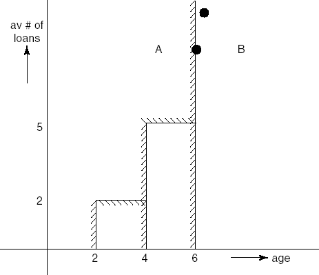
An obvious test technique for this requirement is to use an input from each of these subdomains. If the program follows the logic of the requirement, then test adequacy for that requirement equals path coverage for the corresponding program. However, in error-based testing, we focus on error-prone points and these are often found near the borders of subdomains.
One such test strategy concentrates on ON and OFF points. An ON point is a point on the border of a subdomain. If a subdomain is open with respect to some border, then an OFF point of a border is a point just inside that border. If a subdomain is closed with respect to some border, then an OFF point lies just outside that border. Two adjacent subdomains share the same ON point; they may share the same OFF point. In Figure 13.11, the solid circle on the line age = 6 is an ON point of both A and B, while the circle just off this line is an OFF point of both these subdomains.
Suppose we have subdomains Di, i = 1, ..., n. We may then construct a test set which contains N test cases for ON points of each border B of each subdomain Di, and at least one test case for an OFF point of each border. The resulting test set is called N × 1 domain adequate.
Above, we illustrated this error-based technique in its black-box, specification-based form. The same technique can be applied to program text, though. If a program contains code of the form:
if(x>6) ...else{if(x>4) && (y<5) ...else{if(x>2) && (y ≤ 2) ...else... } }
then we may identify the same four subdomains and use the same technique to test for boundary cases. In fact, this technique is just a systematic way to do what experienced programmers have done for a long time: test for boundary values, such as 0, nil, lists with 0 or 1 element, and so on.
Most test techniques are heuristic in nature and lack a sound theoretical basis. Manual test techniques rely heavily on the qualities of the participants in the test process. But even the systematic approaches taken in functional and structural test techniques have a rather weak underpinning and are based on assumptions that are generally not true.
Experiments show that it is sometimes deceptively simple to make a system produce faults or even let it crash. (Miller et al., 1990) describe one such experiment, in which they were able to crash or hang approximately 30% of the UNIX utilities on seven versions of the UNIX operating system. The utilities tested included commonly used text editors and text formatters.
Similar results have been obtained in mutation analysis experiments. In one such experiment (Knight and Ammann, 1985), 17 programs developed by different programmers from one specification were used. These programs had all been thoroughly tested. Some of them had successfully withstood one million tests. For each of those programs, 24 mutants were created, each mutant containing one seeded fault. The programs thus obtained were each tested 25 000 times. The results can be summarized as follows:
Some seeded faults were found quickly, some needed quite a few tests, and some remained undetected even after 25 000 tests. This pattern was found for each of the 17 programs.
In some cases, the original program failed, while the modified program yielded the right result.
Several attempts have been made to obtain more insights into the theoretical aspects of test techniques. An example is the research that is aimed at relating different test adequacy criteria. Test adequacy criteria serve as rules used to determine whether or not testing can be terminated. An important issue then is to decide whether one such criterion is 'better' than another. In Section 13.8.1, we compare the strength of a number of test adequacy criteria discussed in previous sections. In Section 13.8.2, we investigate a number of fundamental properties of test adequacy criteria. This type of research is aimed at gaining a deeper insight into properties of different test techniques.
Several experiments have been done to compare different test techniques. Real data on the fault-detection capabilities of test techniques used in a number of projects is also available. In Section 13.8.3, we discuss several of these findings, which may provide some practical insight into the virtues of a number of test techniques.
A question that may be raised is whether, say, the all-uses adequacy criterion is stronger or weaker than the all-nodes or all-edges adequacy criteria. We may define the notion 'stronger' as follows: criterion X is stronger than criterion Y if, for all programs P and all test sets T, X adequacy implies Y adequacy. In the testing literature, this relation is known as 'subsume'. In this sense, the all-edges criterion is stronger than (subsumes) the all-nodes criterion. The all-uses criterion, however, is not stronger than the all-nodes criterion. This is caused by the fact that programs may contain statements which only refer to constants. For the following program:
if(a < b) System.out.println("0");elseSystem.out.println("1");
the all-uses criterion will be satisfied by any non-empty test set, since this criterion does not require that each statement be executed. If we ignore references to constants, the all-uses criterion is stronger than the all-nodes criterion. With the same exception, the all-uses criterion is also stronger than the all-edges criterion.
A problem with any graph-based adequacy criterion is that it can only deal with paths that can be executed (feasible paths). Paths which cannot be executed are known as 'infeasible paths'. Infeasible paths result if parts of the graph are unreachable, as in
if(true) x = 1;elsex = 2;
The else branch is never executed, yet most adequacy criteria require this branch to be taken. Paths that are infeasible also result from loops. If a loop is of the form
for(i = 1; i<10; i++) body
all feasible paths that traverse the resulting cycle in the graph will do so exactly ten times.
There does not exist a simple linear scale along which the strength of all program-based adequacy criteria can be depicted. For the criteria discussed in Sections 13.5 to 13.7, the subsume hierarchy is depicted in Figure 13.12, as far as it is known. An arrow A → B indicates that A is stronger than (subsumes) B. In most cases, the subsume relation holds for both the feasible and not feasible versions of the criteria. Arrows adorned with an asterisk denote relations which hold only for the not feasible version.
The subsume relation compares the thoroughness of test techniques, not their ability to detect faults. If an adequacy criterion is used to generate the next test case, the subsume relations of Figure 13.12 do not necessarily imply better fault detection. However, if some other tool is used to generate test cases, and the criterion is only used to decide when to stop testing, a stronger adequacy criterion implies better fault detection as well.
The theoretical upper bounds for the number of test cases needed to satisfy most of the coverage-based adequacy criteria are quadratic or exponential. Empirical studies, however, show that, in practice, these criteria are usually linear in the number of conditional statements.
A major problem with any test technique is to decide when to stop testing. As noted, functional and structural test techniques provide only weak means for doing so. Weyuker (1988) provides an interesting set of properties of test adequacy criteria. Although it is intuitively clear that any test adequacy criterion should satisfy all of the properties listed, it turns out that even some of the well-known test techniques such as all-nodes coverage and all-edges coverage fail to satisfy several of them.
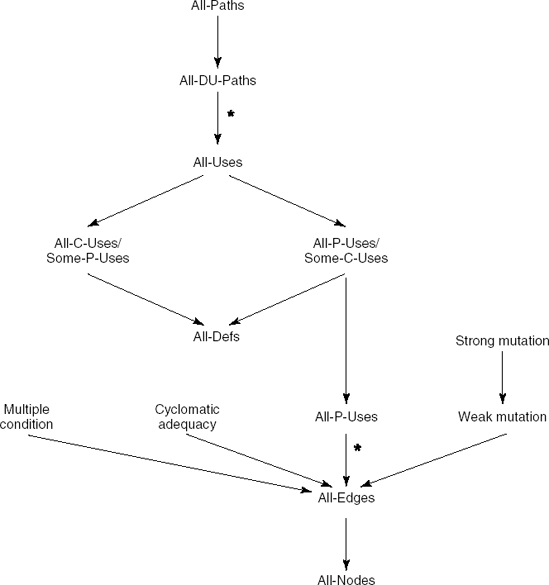
The characteristics identified relate to program-based adequacy criteria, i.e. criteria that involve the program's structure. The first four criteria, however, are fairly general and should apply to any test adequacy criterion. The following 11 properties are identified in (Weyuker, 1988):[24]
Applicability property For every program, there exists an adequate test set. Exhaustive testing obviously satisfies this criterion but, in general, we will look for a reasonably sized test set. Both all-nodes and all-edges coverage criteria do not fulfill this property. If the program contains unexecutable code, there are no tests to cover those parts of the program.
Non-exhaustive applicability property This property says that, even if exhaustive testing may be required in some cases, a criterion should certainly not require exhaustive testing in all circumstances.
Monotonicity property This property states that once a program has been adequately tested, running some additional tests can do no harm. Obviously, the additional tests may reveal further faults, but this does not deem the original test set inadequate. It merely improves the quality of the test process.
Inadequate empty set property The empty test set is not an adequate test set for any program. A test adequacy criterion should measure how well the testing process has been conducted. If a program has not been tested at all, it certainly has not been adequately tested.
Antiextensionality property This property states that semantic equivalence is not sufficient to imply that the programs are to be tested in the same way. For instance, routines BubbleSort and QuickSort are likely to require different test sets. This property is specific for program-based adequacy criteria, which depend on the implementation rather than the function being implemented. In a specification-based approach, this property need not hold.
General multiple change property Whereas the previous property states that semantic 'closeness' is not sufficient to imply that two programs can be tested in the same way, this property states that syntactic closeness is not sufficient either. Programs are said to be syntactically close if they have the same structure and the same data flow characteristics. This is the case, for instance, when some of the relational or arithmetic operators in those programs differ. Though the shape of these programs is the same, testing them on the same data may well cause different paths through the flow graph being executed.
Antidecomposition property This property states that if a component is adequately tested in one environment, this does not imply that it is adequately tested for some other environment. Put in other words: if some assembly of components is adequately tested, this does not imply that the individual components have been adequately tested as well. For example, a sorting routine may well be adequately tested in an environment where the size of the array is always less than ten. If we move that routine to an environment which requires much larger arrays to be sorted, it must be tested anew in that environment.
Anticomposition property This property reflects just the opposite: even if components have been adequately tested in isolation, we still have to test their composition in order to ascertain that their interfaces and interactions work properly.
Renaming property If two programs differ only in inessential ways, as is the case when different variable names are used, then an adequate test set for one of these programs also suffices for the other.
Complexity property Intuitively, more complex programs require more testing. This property reflects this intuition by stating that for every program there exist other programs that require more testing.
Statement coverage property One central property of program-based adequacy criteria is that they should at least cause every executable statement of the program to be executed.
As noted, the all-nodes and all-edges coverage metrics fail to satisfy the applicability criterion. This is rather unsatisfactory, since it implies that we may not be able to decide whether testing has been adequate. If 50% coverage has been obtained using either of these criteria, we do not know whether additional tests will help. It may be that the other 50% of the statements or branches is not executed by any input.
Both the all-nodes and all-edges criteria do not satisfy the antidecomposition and anticomposition criteria either. For example, if all statements of individual components are executed using some given test set, then this same test set is likely to satisfy that criterion on their composition. Further research along these lines is expected to deepen our insight into what test techniques may or may not accomplish.
When one vacuums a rug in one direction only, one is likely to pick up less dirt than if the vacuuming occurs in two directions.
(Cha et al., 1988, p. 386)
The most common techniques for unit testing have been discussed in the previous sections. The effectiveness of those techniques is discussed by Basili and Selby (1987). They describe an experiment in which both professional programmers and students participated. Three techniques were compared:
stepwise abstraction;
functional testing based on equivalence classes and boundary value analysis (see Section 13.7);
structural testing with 100% statement coverage.
Basili and Selby compared the effectiveness of these techniques as regards detecting faults, the associated costs, and the kinds of faults found. Some of the results of this experiment were:
The professional programmers detected more faults with stepwise abstraction. Also, they did so faster than with the other techniques. They discovered more faults with functional testing than with structural testing. The speed with which they did so did not differ.
In one group of students, the various test techniques yielded the same results as regards the number of faults found. In a second group, structural testing turned out to be inferior to the other techniques. The speed with which faults were detected did not differ.
The number of faults found, the speed of fault detection, and the total effort needed depended upon the kind of program being tested.
More interface faults were found with stepwise abstraction.
More faults in the control structure were found with functional testing.
Other experiments also indicate that there is no uniform 'best' test technique. Different test techniques tend to reveal different types of fault. The use of multiple test techniques certainly results in the discovery of more faults. It is difficult though to ascribe the discovery of faults to the use of a specific technique. It may well be that the mere fact that test techniques force us to pay systematic attention to the software is largely responsible for their success.
Several studies have reported on the fault-detection capabilities of (Fagan) inspections. Myers (1988) reports that about 85% of the major errors in the Space Shuttle software were found during early inspections. Inspections have been found to be superior to other manual techniques such as walkthroughs. Inspections were also found to have the additional benefit of improving both quality and productivity. There is some controversy about the added value of group meetings.
Finally, there is ample empirical evidence that early attention to fault detection and removal really pays off. Boehm's data, presented in the introduction to this chapter, can be augmented by other results, such as those of Collofello and Woodfield (1989). His data stems from a large real-time software project, consisting of about 700 000 lines of code developed by over 400 people. Some of his findings are reproduced in Table 13.6. For example, of the 676 design faults that could have been caught, 365 were caught during the design review (= 54%). The overall design review efficiency was not much different from code review efficiency, while the testing phase was somewhat less efficient. The latter is not all that surprising, since the design and code reviews are likely to have removed many of the faults that were easy to detect. These results again suggest that the use of multiple techniques is preferable to the use of a single technique.
Table 13.6. Fault-detection efficiency
% design faults found | % coding faults found | Combined efficiency | |
|---|---|---|---|
Design review | 54 | - | 54 |
Code review | 33 | 84 | 64 |
Testing | 38 | 38 | 38 |
The results become much more skewed if we take into account the cost-effectiveness of the different test techniques. The cost-effectiveness metric used is the ratio of 'costs saved by the process' to 'costs consumed by the process'. The costs saved by the process are the costs that would have been spent if the process had not been performed and faults had to be corrected later. The cost-effectiveness results found in this study are given in Table 13.7. These results indicate that, for every hour spent in design reviews and correcting design faults, more than eight hours of work are saved. The cost-effectiveness of the testing phase itself is remarkably low. This is not really surprising, since much time is wasted during the actual testing phase in performing tests that do not reveal any faults. These findings once more confirm the statement that early testing really pays off.
During the design phase, the system to be built has been decomposed into components. Generally, these components form some hierarchical structure. During testing, we often let ourselves be led by this structure. We do not immediately start to test the system as a whole but start by testing the individual components (called unit testing). These components are incrementally integrated into a system. Testing the composition of components is called integration testing.
In doing this, we may take one of two approaches. In the first approach, we start by testing the low-level components, which are then integrated and coupled with components at the next higher level. The subsystem thus obtained is tested next. Then gradually we move towards the highest-level components. This is known as bottom-up testing. The alternative approach is top-down testing. In top-down testing, the top-level components are tested first and are gradually integrated with lower-level components.
In bottom-up testing, we often have to simulate the environment in which the component being tested is to be integrated. Such an environment is called a test driver. In top-down testing the opposite is true: we have to simulate lower-level components through test stubs.
Both methods have advantages and disadvantages. For instance, in bottom-up testing it may be difficult to get a sound impression of the final system during the early stages of testing because whilst the top-level components are not integrated, there is no system, only bits and pieces. With top-down testing, on the other hand, writing the stubs can be rather laborious. If the implementation strategy is one whereby a skeletal system is built first and then populated with components, this skeletal system can be used as a test driver and the order of testing then becomes much less of an issue.
In practice, it is often useful to combine both methods. It is not necessarily the case that some given design or implementation technique drives us in selecting a particular test technique. If the testing is to partly parallel the implementation, ordering constraints induced by the order of implementation have to be obeyed, though.
The program-based adequacy criteria make use of an underlying language model. Subtle differences in this underlying model may lead to subtle differences in the resulting flow graphs as used in coverage-based criteria, for instance. Roughly speaking, the results reported hold at the level of a procedure or subroutine in languages such as FORTRAN, Pascal, and so on.
As a consequence, the corresponding test techniques apply at the level of individual methods in object-oriented programs. Testing larger components of object-oriented programs, such as parameterized classes or classes that inherit part of their functionality from other classes, resembles regression testing as done during maintenance. We then have to decide how much retesting should be done if methods are redefined in a subclass or a class is instantiated with another type as a parameter.
Other forms of testing exist besides unit testing and integration testing. One possibility is to test the whole system against the user documentation and requirements specification after integration testing has finished. This is called the system test. A similar type of testing is often performed under supervision of the user organization and is then called acceptance testing. During acceptance testing, emphasis is on testing the usability of the system, rather than compliance of the code against some specification. Acceptance testing is a major criterion upon which the decision to accept or reject a system is based. In order to ensure proper delivery of all necessary artifacts of a software development project, it is useful to let the future maintenance organization have a right of veto in the acceptance-testing process.
If the system has to become operational in an environment different from the one in which it has been developed, a separate installation test is usually performed.
The test techniques discussed in the previous sections are often applied during unit and integration testing. When testing the system as a whole, the tests often use random input, albeit that the input is chosen such that it is representative of the system's operational use. Such tests can also be used to quantitatively assess the system's reliability. Software reliability is the topic of Section 13.10.
The use of random input as test data has proven to be successful in the Cleanroom development method. In several experiments, it was found that aselect testing resulted in a high degree of statement and branch coverage. If a branch was not executed, it often concerned the treatment of an exceptional case.
In much of this book the reader will find references to the fact that most software does not function perfectly. Faults are found in almost every run-of-the-mill software system: the software is not 100% reliable. In this section we concentrate on quantitative, statistical notions of software reliability.
One benefit of such information is that it can be put to use in planning our maintenance effort. Another reason for collecting reliability information could be contractual obligations regarding a required reliability level. Software for telephone-switching systems, for instance, requires such quantitative knowledge of the system's expected availability. We need to know the probability of wrong connections being due to faults in the software.
A second application of reliability data is found in testing. A major problem with testing is deciding when to stop. One possibility is to base this decision on reaching a certain reliability level. If the required reliability level is not reached, we need an estimate of the time it will take to reach that level.
In order to be able to answer this type of question, a number of software reliability models have been developed which strongly resemble the well-known hardware reliability models. These are statistical models where the starting point is a certain probability distribution for expected failures. The precise distribution is not known in advance. We must measure the points in time at which the first n failures occur and look for a probability distribution that fits those data. We can then make predictions using the probability distribution just obtained.
In this section, we concentrate on two models which are not too complicated and yet yield fairly good results: the basic execution time model and the logarithmic Poisson execution time model.
The goal of many test techniques discussed in this chapter is to find as many faults as possible. What we in fact observe are manifestations of faults, i.e. failures. The system fails if the output does not meet the specification. Faults in a program are static in nature, failures are dynamic. A program can fail only when it is executed. From the user's point of view, failures are much more important than faults. For example, a fault in a piece of software that is never, or hardly ever, used is, in general, less important than a fault which manifests itself frequently. Also, one fault may show up in different ways and a failure may be caused by more than one fault.
In the following discussion on reliability, we are not concerned with the expected number of faults in a program. Rather, the emphasis is on the expected number of failures. The notion of time plays an essential role. For the moment, we define reliability as the probability that the program will not fail during a certain period of time.
The notion of time deserves further attention. Ultimately, we are interested in statements regarding calendar time. For example, we might want to know the probability that a given system will not fail in a one-week period or we might be interested in the number of weeks of system testing still needed to reach a certain reliability level.
Both models discussed below use the notion of execution time. Execution time is the time spent by the machine actually executing the software. Reliability models based on execution time yield better results than those based on calendar time. In many cases, an a posteriori translation of execution time to calendar time is possible. To emphasize this distinction, execution time is denoted by t and calendar time by t.
The failure behavior of a program depends on many factors: quality of the designers, complexity of the system, development techniques used, etc. Most of these cannot adequately be dealt with as variables in a reliability model and therefore are assumed to be fixed. For this reason, reliability, when discussed in this section, always concerns a specific project.
Some factors affecting failure behavior can be dealt with, though. As remarked, the models discussed are based on the notion of execution time. This is simple to measure if we run one application on a stand-alone computer. Translation between machines that differ in speed can be taken care of relatively easily. Even if the machine is used in multiprogramming mode, translation from the time measured to proper execution time may be possible. This is the case, for instance, if time is relatively uniformly distributed over the applications being executed.
The input to a program is also variable. Since we estimate the model's parameters on the basis of failures observed, the predictions made only hold insofar as future input resembles the input which led to the observed failure behavior. The future has to resemble the past. In order to get reliable predictions, the tests must be representative of the later operational use of the system. If we are able to allocate the possible inputs to different equivalence classes, simple readjustments are possible here too.
We may summarize this discussion by including the environment in the definition of our notion of software reliability. Reliability then is defined as the probability that a system will not fail during a certain period of time in a certain environment.
Finally, software systems are not static entities. Software is often implemented and tested incrementally. Reliability of an evolving system is difficult to express. In the ensuing discussion, we therefore assume that our systems are stable over time.
We may characterize the failure behavior of software in different ways. For example, we may consider the expected time to the next failure, the expected time interval between successive failures, or the expected number of failures in a certain time interval. In all cases, we are concerned with random variables, since we do not know exactly when the software will fail. There are at least two reasons for this uncertainty. Firstly, we do not know where the programmer made errors. Secondly, the relation between a certain input and the order in which the corresponding set of instructions is being executed is not usually known. We may therefore model subsequent failures as a stochastic process. Such a stochastic process is characterized by, amongst other things, the form and probability distribution of the random variables.
When the software fails, we try to locate and repair the fault that caused this failure. In particular, this situation arises during the test phase of the software life cycle. Since we assume a stable situation, the application of reliability models is particularly appropriate during system testing, when the individual components have been integrated into one system. This system-test situation, in particular, is discussed below.
In this situation, the failure behavior does not follow a constant pattern but changes over time, since faults detected are subsequently repaired. A stochastic process whose probability distribution changes over time is called non-homogeneous. The variation in time between successive failures can be described in terms of a function μ(τ) which denotes the average number of failures until time τ. Alternatively, we may consider the failure intensity function λ(τ), the average number of failures per unit of time at time τ. λ(τ), then, is the derivative of μ(τ). If the reliability of a program increases through fault correction, the failure intensity will decrease.
The relationship between λ(τ), μ(τ) and τ is graphically depicted in Figure 13.13. The models to be discussed below, the basic execution time model (BM) and the logarithmic Poisson execution time model (LPM), differ in the form of the failure intensity function λ (τ).
Both BM and LPM assume that failures occur according to a non-homogeneous Poisson process. Poisson processes are often used to describe the stochastic behavior of real-world events. Examples of Poisson processes are: the number of telephone calls expected in a given period of time or the expected number of car accidents in a given period of time. In our case, the processes are non-homogeneous, since the failure intensity changes as a function of time, assuming a (partly) successful effort to repair the underlying errors.
In BM, the decrease in failure intensity, as a function of the number of failures observed, is constant. The contribution to the decrease in failure intensity thus is the same for each failure observed. In terms of the mean number of failures observed (μ), we obtain:
Here, λ0 denotes the initial failure intensity, i.e. the failure intensity at time 0. υ0 denotes the number of failures observed if the program is executed for an infinite time period. Note that, since λ is the derivative of μ and both are functions of τ, λ in fact only depends on τ. We return to this later.
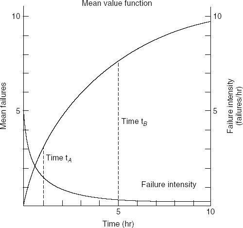
Figure 13.13. Failure intensity λ(τ) and mean failures μ(τ) as functions of τ (Source: J.D. Musa, A. Iannino and K. Okumoto, Software Reliability, ©1987, McGraw-Hill Book Company. Reproduced by permission of McGraw-Hill, Inc.)
In LPM, the first failure contributes more to the decrease in failure intensity than any subsequent failures. More precisely, the failure intensity is exponential in the number of failures observed. We then get:
In this model, θ denotes the decrease in failure intensity. For both models, the relation between λ and μ is depicted in Figure 13.14. (Note that the two curves intersect in this picture. This need not necessarily be the case. It depends on the actual values of the model parameters.)
Both models have two parameters: λ0 and υ0 for BM; and λ0 and θ for LPM. These parameters have yet to be determined, for instance from the observed failure behavior during a certain period of time.
We can explain the shape of these functions as follows: given a certain input, the program in question will execute a certain sequence of instructions. A completely different input may result in a completely different sequence of instructions to be executed. We may partition all possible inputs into a number of classes such that input from any one class results in the execution of the same sequence of instructions. Some example classes could be a certain type of command in an operating system or a certain type of transaction in a database system.
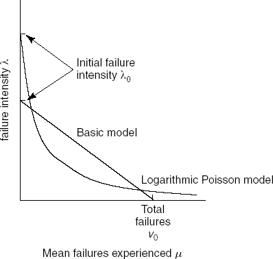
Figure 13.14. Failure intensity λ as a function of μ (Source: J.D. Musa, A. Iannino and K. Okumoto, Software Reliability, ©1987, McGraw-Hill Book Company. Reproduced by permission of McGraw-Hill, Inc.)
The user selects input from the various possible classes according to some probability distribution. We define the operational profile as the set of possible input classes together with the probabilities that input from those classes is selected.
The basic execution time model implies a uniform operational profile. If all input classes are selected equally often, the various faults have an equal probability of manifesting themselves. Correction of any of those faults then contributes the same amount to the decrease in failure intensity. It has been found that BM still models the situation fairly well in the case of a fairly non-uniform operational profile.
With a strong non-uniform operational profile, the failure intensity curve has a convex shape, as in LPM. Some input classes are, then, selected relatively often. As a consequence, certain faults show up earlier and are corrected sooner. These corrections have a larger impact on the decrease in failure intensity.
In both models, λ and μ are functions of τ (execution time). Furthermore, failure intensity λ is the derivative of mean failures μ. For BM, we may therefore write
as
Solving this differential equation yields
and
In a similar way, we obtain for LPM:
and
For LPM, the expected number of failures in infinite time is infinite. Obviously, the number of failures observed during testing is finite.
Both models allow that fault correction is not perfect. In BM the effectiveness of fault correction is constant, though not necessarily 100%. This again shows up in the linearity of the failure intensity function. In LPM, the effectiveness of fault correction decreases with time. Possible reasons could be that it becomes increasingly more difficult to locate the faults, for example because the software becomes less structured or the personnel less motivated.
If the software is operational and faults are not being corrected, the failure intensity remains constant. Both models then reduce to a homogeneous Poisson process with failure intensity λ as the parameter. The number of failures expected in a certain time period follows a Poisson distribution. The probability of exactly n failures being observed in a time period of length τ is then given by
The probability of 0 failures in a time frame of length τ then is P0(τ) = exp(-λτ). This is precisely what we earlier denoted by the term software reliability.
Given a choice of either of the models BM or LPM, we are next faced with the question of how to estimate the model's parameters. We may do so by measuring the points in time at which the first N failures occur. This gives us points T1, ..., Tn. These points can be translated into pairs (τ, μ(τ)). We may then determine the model's parameters so that the resulting curve fits the set of measuring points. Techniques such as Maximum Likelihood or Least Squares are suited for this.
Once these parameters have been determined, predictions can be made. For example, suppose the measured data results in a present failure intensity λP and the required failure intensity is λF. If we denote the additional test time required to reach failure intensity λF by Δτ, then we obtain for BM:
And for LPM we get:
Obviously, we may also start from the equations for μ. We then obtain estimates for the number of failures that have yet to be observed before the required failure intensity level is reached.
For BM, this extrapolation is graphically depicted in Figure 13.15. Since estimating the model's parameters is a statistical process, we do not actually obtain one solution. Rather, we get reliability intervals. Such a reliability interval denotes the interval which contains a parameter with a certain probability. For example, λ0 may be in the interval [80,100] with probability 0.75. So the curve in Figure 13.15 is actually a band. The narrower this band is, the more accurately the parameters have been estimated for the same reliability of the interval. In general, the estimates are more accurate if they are based on more data.
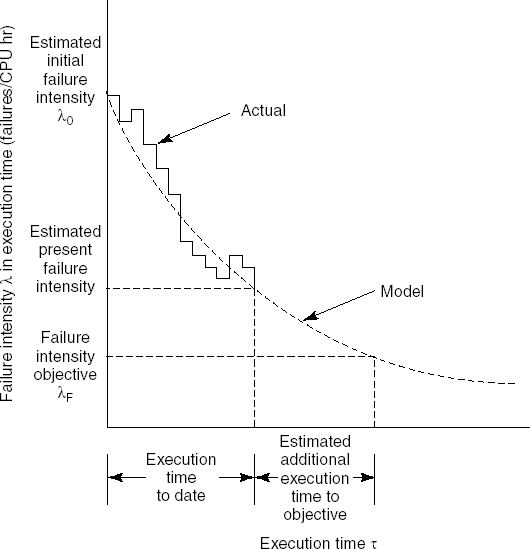
Figure 13.15. A conceptual view of the parameter-estimating process (Source: J.D. Musa, A. Iannino and K. Okumoto, Software Reliability, ©1987, McGraw-Hill Book Company. Reproduced by permission of McGraw-Hill, Inc.)
In the above discussion, we used the notion of execution time. That calendar time is a less useful notion on which to base our model can be seen as follows: suppose the points in time at which the first N failures occurred were expressed in terms of calendar time. Suppose also that we try to correct a fault as soon as it manifests itself. If the manpower available for fault correction is limited and is capable of solving a fixed number of problems per day, the failure intensity will be constant if it is based on calendar time. We do not, then, observe any progress.
Quite a few reliability models have been proposed in the literature. The major differences concern the total number of failures (finite or infinite) that can be experienced in infinite time and the distribution of the failures experienced at a given point in time (for example, Poisson, and binomial).
An important question then arises as to which model to choose. By studying a number of failure data sets, it has been observed that no one model is consistently the best. We therefore have to look for the model that gives the best prediction on a project-by-project basis. Since we do not know in advance which model will perform best, it is wise to adopt an eclectic approach, and use a number of different models simultaneously.
In this chapter, we discussed a great number of test techniques. We emphasized the importance of early fault detection. It is important to pay attention to testing during the early stages of the software development process. Early testing activities are the ones that are most cost effective. Early testing activities provide opportunities to prevent errors from being made in the first place. An extreme form of this is test-driven development, where writing tests is the very first thing we do.
In practice, the various manual test techniques seem to be used most often. They turn out to be at least as successful as the various structural and functional techniques. Inspections in particular have been found to be a very cost-effective test technique. Next to the test techniques used, a major element in software fault detection and removal is the choice of personnel — some people are significantly better at finding and removing faults than others.
Since exhaustive testing is generally not feasible, we have to select an adequate set of test cases. Test techniques can be classified according to the criterion used to measure the adequacy of a test set. Three broad categories of test adequacy criteria can be distinguished:
coverage-based testing, in which testing requirements are specified in terms of the coverage of the product to be tested, for example, the percentage of statements executed;
fault-based testing, in which the focus is on detecting faults, for example, the percentage of seeded faults detected;
error-based testing, which focuses on testing error-prone points, such as 0, 1, or the upper bound of an array.
A test adequacy criterion can be used as a stopping rule, a measurement instrument, or a generator of test cases. Test adequacy criteria and the corresponding test techniques can be viewed as two sides of the same coin. A coverage-based test technique makes it easy to measure coverage-based criteria, but does not help us in assessing whether all error-prone points have been tested.
Experimental evaluations show that there is no uniform best test technique. Different techniques tend to reveal different types of error. It is therefore wise to 'vacuum the carpet in more than one direction'.
One line of research addresses the relative power of test adequacy criteria. A well-known measure for comparing program-based test adequacy criteria is the subsume relation: criterion X subsumes Y if, for all programs P and all test sets T, X adequacy implies Y adequacy. Many of the well-known adequacy criteria have been related to one another in a subsume hierarchy.
As with any other life cycle activity, testing has to be carefully planned, controlled, and documented. Some of the IEEE Standards provide useful guidelines for doing this (IEEE829, 1998; IEEE1012, 2004).
Section 13.10 was devoted to a discussion of how to quantitatively estimate the reliability of a piece of software. The currently available software reliability models are limited in their immediate practical value. In particular, no model consistently performs best.
Well-known textbooks on testing are (Myers, 1979) (and its updated version (Myers, 2004)), (Beizer, 1995) and (Copeland, 2003). Whittaker (2000) gives a concise overview of the field. For a further discussion of safety issues, see (Leveson, 1991). Fault-tree analysis is discussed in (Leveson, 1986). (Zhu et al., 1997) give a very good overview of the types of test strategy discussed in Sections 13.5 to 13.7 and the associated adequacy criteria. Rothermel and Harrold (1996) and Harrold (1999) give a very good overview of regression test techniques. Testing object-oriented software is addressed in (Binder, 2000).
The first attempts at developing some theory on testing date back to the 1970s and 80s (Goodenough and Gerhart, 1975), (Howden, 1982), and (Howden, 1985). Thereafter, much of that research has been directed towards finding and relating test adequacy criteria (Weyuker, 1988), (Clarke et al., 1989), (Weyuker, 1990), (Frankl and Weyuker, 1993a), (Frankl and Weyuker, 1993b), (Parrish and Zweben, 1995), and (Zhu, 1996). Experimental evaluations of test adequacy criteria can be found in (Frankl and Weiss, 1993), (Weyuker, 1993), (Offutt and Lee, 1994), (Harrold et al., 1997), and (Frankl et al., 1997). Experiments that compare manual and functional or structural test techniques are reported upon in (Basili and Selby, 1987), (Kamsties and Lott, 1995), and (Wood et al., 1997). (Juristo et al., 2004) give an overview of 25 years of testing technique experiments.
The Cleanroom development method is described in (Selby et al., 1987) and (Mills et al., 1987). Experiences with Cleanroom are discussed in (Currit et al., 1986) and (Trammell et al., 1992). Stepwise abstraction is described in (Linger et al., 1979).
Beck (2003) describes test-driven development. Janzen and Saiedian (2005) give a somewhat wider perspective on its potential. Hunt and Thomas (2003) is one of the many textbooks describing JUnit. Effects of test-driven development on productivity and errors are reported in (Maximilien and Williams, 2003) and (Erdogmus et al., 2005).
Inspections were introduced by Fagan in the 1970s (Fagan, 1976, 1986). Gilb and Graham (1993) is a textbook on inspections; Wiegers (2002) is a textbook on peer reviews. There have been many experimental evaluations of inspections; see for instance (Knight and Myers, 1993), (Weller, 1993), (Grady and van Slack, 1994), (Porter et al., 1995), (Porter et al., 1997), (Porter et al., 1998), and (Biffl and Halling, 2002). Parnas and Lawford (2003a) and Parnas and Lawford (2003b) are introductions to two companion special journal issues on software inspections. (Ciolkowski et al., 2003) discuss the state of the art in software reviews.
The basic execution time model and the logarithmic Poisson execution time model are extensively discussed, and compared with a number of other models, in (Musa et al., 1987). (Lyu, 1995) is a very comprehensive source on software reliability. Experiences with software reliability modeling are reported in (Jeske and Zhang, 2005). Whittaker and Voas (2000) give criteria other than time and operational profile that affect reliability.
Describe the following categories of test technique: coverage-based testing, fault-based testing, and error-based testing.
What assumptions underlie the mutation testing strategy?
What is the difference between black-box testing and white-box testing?
Define the following terms: error, fault, and failure.
What is a Fagan inspection?
What is test-driven development?
Define the following categories of control-flow coverage: all-paths coverage, all-edges coverage, all-statements coverage.
Consider the following routine (in Modula-2):
procedureSiftDown(varA:array ofinteger; k, n: integer);varparent, child, insert, Ak: integer;beginparent:= k; child:= k + k; Ak:= A[k]; insert:= Ak;loopifchild>nthen exit end;ifchild<nthenifA[child]>A[child+1]thenchild:= child+1endend;ifinsert<=A[child]then exitelseA[parent]:= A[child]; parent:= child; child:= child + childendend; A[parent]:= AkendSiftDown;(This operation performs the sift-down operation for heaps; if necessary, you may consult any text on data structures to learn more about heaps.) The routine is tested using the following input:
n = 5, k = 2,
A[1] = 80, A[2] = 60, A[3] = 90, A[4] = 70, A[5] = 10.
Will the above test yield 100% statement coverage? If not, provide one or more additional test cases such that 100% statement coverage is obtained.
For the example routine from Exercise 9, construct a test set that yields 100% branch coverage.
For the example routine from Exercise 9, construct a test set that achieves all-uses coverage.
Consider the following two program fragments:
Fragment 1:found = false; counter = 1;while((counter<n) && (!found)) {if(table[counter] == element) found:= true; counter = counter + 1; };if(found) System.out.println("found");elseSystem.out.println("not found");Fragment 2:found = false; counter = 1;while((counter<n) && (!found)) { found = table[counter] == element; counter = counter + 1 };if(found) System.out.println("found");elseSystem.out.println("not found");Can the same test set be used if we wish to achieve 100% branch coverage for both fragments?
What is mutation testing?
Which assumptions underlie mutation testing? What does that say about the strengths and weaknesses of this testing technique?
When is one testing technique stronger than another?
What is the difference between a system test and an acceptance test?
Contrast top-down and bottom-up integration testing.
What is the major difference between the basic execution time model and the logarithmic Poisson execution time model of software reliability?
Give a definition of software reliability. Give a rationale for the various parts of this definition.
Why is it important to consider the operational profile of a system while assessing its reliability?
Can you think of reasons why reliability models based on execution time yield better results than those based on calendar time?
Can software reliability be determined objectively?


public staticvoid selection_sort (int a, int n) { int i, j, small, temp;for(i = 0; i<n-2; i++) { small = i;for(j = i+1; j<n-1; j++)if(a[j]<a[small]) small = j; temp = a[i]; a[i] = a[small]; a[small] = temp; } }Determine the function (by means of pre- and postconditions) of this routine using stepwise abstraction.
an empty array;
an array of length 1;
a sorted array of length 10;
an array of 10 elements that all have the same value;
an array of length 10 with random elements.
Which of these mutants stay alive? What does this tell you about the quality of these tests?
functional or structural testing,
correctness proofs,
random testing, and
inspections
for fault finding and confidence building.
[22] The IEEE Standard Glossary of Software Engineering Terminology (IEEE610, 1990) gives four definitions of the word 'error'. To distinguish between these definitions, the words 'error', 'fault', 'failure' and 'mistake' are used. The word 'error' in the Glossary is used to denote a measurement error, while 'mistake' is used to denote a human error. Though 'mistake' has the advantage of being less condemning, we follow the accepted software engineering literature in this respect. Our definitions of 'fault' and 'failure' are the same as those in the Glossary.
[23] One way of creating a non-threatening atmosphere is to always talk about 'problems' rather than 'faults'.
[24] Reproduced by permission of the Association for Computing Machinery, Inc.