10

Introduction to Petri Nets

10.1 INTRODUCTION TO SIMPLE PETRI NETS

The Petri net is a state diagram that can be used to describe the behaviour of both sequential and parallel systems. It was initially conceived by Karl Petri in the 1960s and has had a good following of academics ever since. There is a website devoted to all things Petri at http://www.informatik.unihamburg.de/TGI/PetriNets/.

Petri nets are often used as a tool to study the behaviour of parallel and concurrent systems (not necessarily electrical). They have also been used to study parallel and concurrent programming methods. In recent years, researchers have shown [1] how the Petri net can be used to develop and synthesize electronic FSM systems, in a similar way to how synchronous and asynchronous systems can be developed and synthesized. The main reason for employing Petri nets is the ability to create parallel systems. The following method makes use of material with permission from [1].

Figure 10.1 illustrates a two-state diagram and its Petri net equivalent. In a Petri net, the ‘state’ is represented by a ‘placeholder’ and the ‘transitional lines’ between states are represented by ‘arcs’ that connect the placeholder (P1 and P2) to transition points (T1 and T2). The inputs along the transitional lines of a state diagram are placed against the transition points along the connecting arcs that link one placeholder to another in a Petri net.

The Petri net uses a memory element to represent each placeholder (rather like in a One Hot state diagram – as illustrated in Figure 10.1). However, in Petri nets used to represent parallel systems, there can be more than one active placeholder (whereas in a state diagram only one state can be active at any one time). For this reason, a Petri net needs some way to show which of its placeholders are active. This is done by using a ‘token’ to represent an active placeholder and by placing a ‘dot’ in the placeholder that is active.

In Figure 10.1, placeholder P1 is active, since it has a token, and placeholder P2 is not active and, hence, does not have a token.

A brief explanation of the behaviour of the Petri net in Figure 10.1 follows.

Initially, a token is in placeholder P1 (via initialization logic to be explained later). When the input x becomes active (x = 1) the transition T1 will fire, and the token will move (following the arc path) to placeholder P2, where it will remain (because T2 is not able to fire since x is still 1), as illustrated in Figure 10.2.

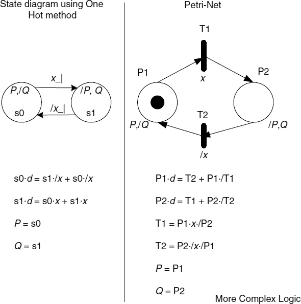
Figure 10.1 Comparison between a state diagram and Petri net with respective equations.

It should be noted that transition T1 will only fire when x = 1 and a clock pulse occurs. Note also that outputs P = 0 and Q = 1 in P2, so outputs are following a Moore-type model. When x = 0 and the next clock pulse occurs, the token will pass back to P1, as shown in Figure 10.1.

The syntheses for this Petri net are based upon the equations shown in Figure 10.1. There are three basic equation types:

• placeholder equations;
• transient equations;
• output equations.

The placeholder equations follow the same format as the sequential equations for an event-driven state machine. This is best described in terms of the Petri net in Figure 10.1, shown in Equation (10.1). The Petri-net equations define the input to a D-type flip-flop, hence the ‘P · d’ on the left-hand side.

This is interpreted as: for P1 to get a token, T2 must have fired; or, to hold on to the token, a token must be in P1 and T1 must not have fired.

For P2:

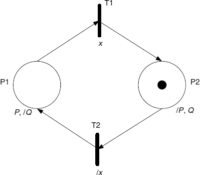
Figure 10.2 Token moved to P2 after T1 fired (x = 1).

The first term T1 on the right-hand side of Equation (10.1) for P1 is, in effect, a turn-on condition for the placeholder P1. The product term P1 · T1 is a hold term for the placeholder.

The transition equations are made up of the conditions necessary for the transition to fire. In the Petri net of Figure 10.1 it can be seen that T1 will only fire if P1 has the token and P2 does not have the token and the input x = 1,. Hence:

In the same way:

There is more to these rules when describing more complex Petri nets, which will be explained later.

Since the placeholder equations of Equations (10.1) and (10.2) are equal to P1 · d and P2 · d respectively, they define the D inputs to D-type flip-flops. This is illustrated in Figure 10.3.

In future examples, the distinction between the left-hand side of a placeholder equation Pn · d will not be made and will take on the appearance of a recursive equation, as in

P1 = T2 + P1 · /T1

P2 = T1 + P2 · /T2.

This implies that the left-hand side is the input to the flip-flop. Reference [1] uses this approach.

Figure 10.3 illustrates the cycle of design from Petri net to equations, and finally synthesized circuit. It implies that once a Petri net has been developed, the synthesization is a systematic application of the rules.

Of course, a PLD device or FPGA could be used and the equations used directly, or the Petri net could be written at the behavioural level in VeriLog HDL.

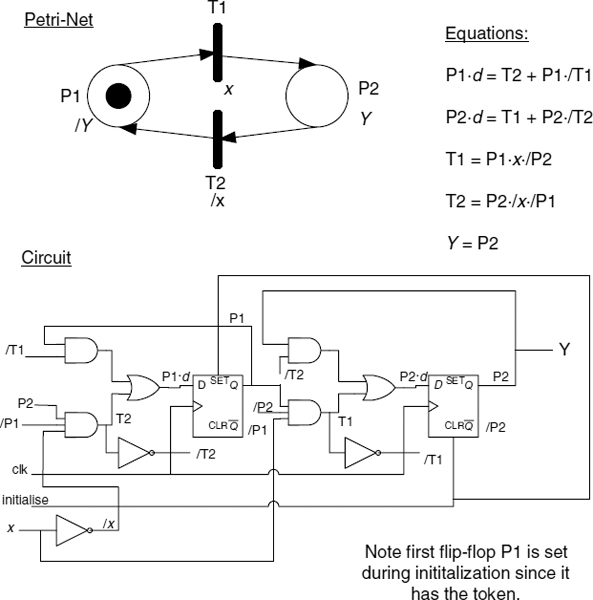
Figure 10.3 Full cycle of design from Petri net to circuit.

In the circuit schematic of Figure 10.3, note the initialization arrangement. This is the same as that used in the One Hot design of state machines. Also note the topological arrangement for the gate logic. The flip-flop output P1 is connected back into the turn off and gate logic; and likewise for the P2 flip-flop. This provides the hold term required to keep the placeholder active.

From this diagram, and the foregoing description of the equations, it can be seen that the flip-flops provide memory for the placeholder element and that a set flip-flop is equivalent to a placeholder with a token and a reset flip-flop is equivalent to a placeholder without a token.

The topological structure of the Petri net can be seen in Figure 10.4:

Tin is the turn-on input, and the feedback from output Pn to the input of the AND gate forms the hold term. The term Tin in Equation (10.5) is of the form:

Tin = input placeholder AND input enable AND NOT output placeholder.

Tout is the turn-off term, which is negated in Equation (10.5). When Tout becomes asserted high, the /Tout input will go low so as to open the feedback hold term to allow the D flip-flop to reset (Tin will not be active at this point).

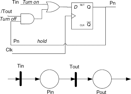
Figure 10.4 Basic topological structure of the Petri net.

A close look at Figure 10.4 shows that the gate logic of the AND and OR gates themselves with the feedback loop would form an asynchronous event cell if the D flip-flop were removed. This is illustrated in Figure 10.5. It can be seen that the Petri net can be synthesized as either a clocked or unclocked (event-driven) system.

Note that if an unclocked (event-driven) system is to be designed, then the gate propagation delays would need to be considered. This is similar to the effects on asynchronous (event-driven) FSMs discussed in Chapter 9.

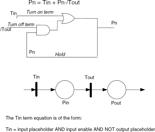
Figure 10.5 Asynchronous (event-driven) Petri net structure.

In Petri nets:

• synchronous designs are clock driven with the D flip-flop elements;
• asynchronous designs are event driven with the D flip-flop elements removed.

There is much research work being carried out on asynchronous Petri nets at a number of universities. You might wish to do a web search using the key words ‘Petri nets’ and ‘C gate’ to obtain further information.

The remainder of this chapter will deal with synchronous clock-driven systems.

To consolidate the ideas discussed so far, a sequential Petri-net controller example will be considered.

10.2 SIMPLE SEQUENTIAL EXAMPLE USING A PETRI NET

A sequential Petri-net controller example is illustrated in Figure 10.6. In this example, a pump P can be turned on by asserting st high to fire T1. After sensor v becomes high, T2 will fire to turn on the motor. Pressing the stop button sp will cause T3 to fire and return the system to placeholder P1, where both motor and pump are turned off.

The equations for this design are shown below, but you might want to cover them up and try to produce them. The equations are illustrated in Figure 10.7, which shows the circuit diagram of the system; initialization circuitry is also shown, with flip flop P1 being set while flip flops P2 and P3 are cleared.

To make this system event driven, the D flip-flops can be removed and the feedback loops completed from the OR gate outputs to the two input AND gates so as to form the event cells for P1, P2, and P3.

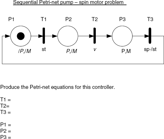
Figure 10.6 Another sequential Petri net design.

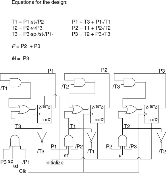
Figure 10.7 Circuit diagram of the Petri net design.

10.3 PARALLEL PETRI NETS

Up to this point, only sequential Petri nets have been considered. However, the main point of using the Petri net is to allow parallel systems to be developed. Therefore, parallel Petri nets will now be discussed.

A parallel Petri net will have parallel paths containing sequences. Figure 10.8 illustrates such a Petri net. In this Petri net there are three parallel paths between the T2 and T5 transitions. P1 and P2 form a sequential path. At T2, they ‘fork’ into three parallel paths. At T5 these parallel paths ‘join’ to form a sequential path again.

When the token reaches P2 and the syn1 input becomes active (high), the token will transfer to P3, P4, and P5, as illustrated in Figure 10.9. The system will now have three event cells (and D flip-flops) set at the same time.

Suppose input p becomes active (high) but input q is not yet active (high). The result will be as shown in Figure 10.10. If, at this point, syn2 were to go active (high), then transition T5 would not fire because the token has not yet reached P7.

A requirement for a Petri net is that all the placeholders merging into a transition (P6, P4, and P7 into T5) must have a token before the transition can fire.

Eventually, when input q = 1, T4 will fire and the token in P5 will move to P7.

In Figure 10.11, all placeholders merging into T5 have tokens; so, whenever syn2 = 1, T5 will fire and the tokens will ‘join’ and P1 will obtain the token again.

Figure 10.8 Petri net with parallel paths.

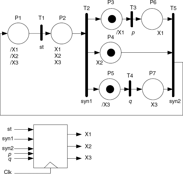
Figure 10.9 Tokens moved into three parallel paths (fork).

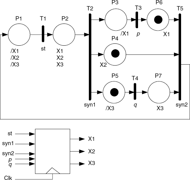
Figure 10.10 Input p = 1, q = 0 with P5, P6, and P4 active, but not P7.

The above discussion has described a mechanism in which sequential flow can become parallel flow and merge back into sequential flow again. Most parallel systems behave in this manner, and the Petri net can be used to model such behaviour. This has been one of the principle uses for Petri nets in the past.

In the example illustrated in Figures 10.8–10.11, the transitions T2 and T5 act as synchronizing points; syn1 (controlling the firing of T2) is used to synchronize the point of ‘fork’, andsyn2 (controlling the firing of T5) is used to synchronize the point of ‘join’. So, in a hardware system, the two signals syn1 and syn2 act as synchronizing points.

However, the Petri net is self-regulating, since all placeholders converging onto a transition must have tokens before the transition can fire.

The equations will now be developed for this example.

First the placeholder terms:

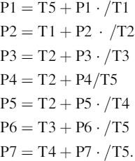
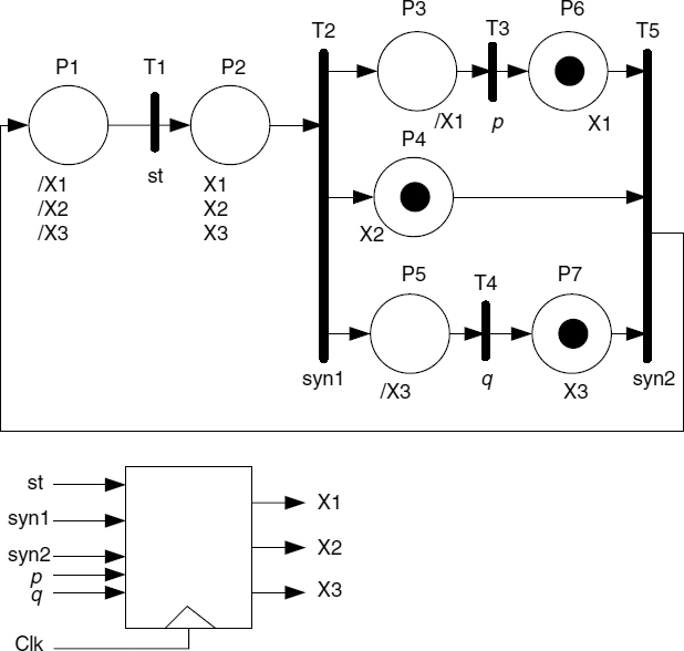
Figure 10.11 T5 can fire whenever input syn2 becomes active (high).

Now the transition terms:

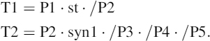
Note here that for T2 to fire there must be a token in placeholder P2, signal syn1 must be active, but none of the P3, P4, or P5 placeholders must be active.

Here, all parallel path placeholders merging onto T5 must have a token. The equations for T2 and T5 need to be noted.

Finally, the outputs can be written as

X1 = P2 + P6

X2 = P2 + P4

X3 = P2 + P7.

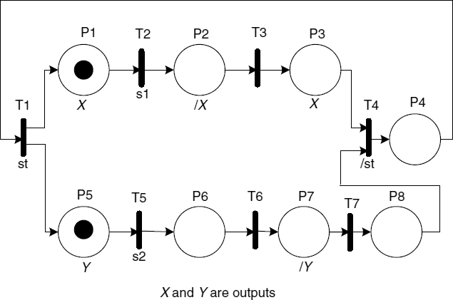
Figure 10.12 Another parallel Petri net example.

10.3.1 Another Example of a Parallel Petri Net

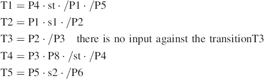
Figure 10.12 illustrates another Petri net example. You might like to try to write down the equations for this one and check the solution with the equations below. The results should be as follows.

The placeholder terms are

P1 = T1 + P1 · /T2

P2 = T2 + P2 · /T3

P3 = T3 + P3 · /T4

P4 = T4 + P4 · /T1

P5 = T1 + P5 · /T5

P6 = T5 + P6 · /T6

P7 = T6 + P7 · /T7

P8 = T7 + P8 · /T4.

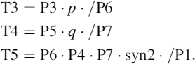
The transitional terms are

T6 = P6 · /P7

T7 = P7 · /P8.

The outputs are

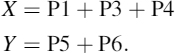
10.4 SYNCHRONIZING FLOW IN A PARALLEL PETRI NET

In the example in Section 10.3, use was made of synchronizing inputs syn1 and syn2 to synchronize the flow from sequential to parallel, and from parallel to sequential. Sometimes, however, there is a need to synchronize between two separate Petri nets. Consider the example in Figure 10.13.

This clearly cannot be done without having some shared communication. It is a classical problem in parallel programming systems. However, in a parallel programming system, a share variable might be considered appropriate. This is dangerous, since this variable could be written to by either of the two parallel entities.

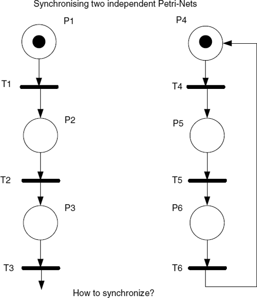
Figure 10.13 Synchronizing two independent Petri nets?

10.4.1 Enabling and Disabling Arcs

In the Petri net there is a way to overcome this problem, using either

• an enabling arc, or
• a disabling arc.

Consider, first, the action of an enabling arc. As can be seen from Figure 10.14, the process made up from P1 to P3 and the process made up from P4 to P6 are totally independent. However, the dashed line from P2 to T5 indicates that there must be a token in P2 in order to enable T5. However, T5 must also have a token in P5 and its go signal must be active (high). So, the condition for T5 to fire will be

This arrangement ensures that both Petri nets are at a particular state in their sequence (P2 and P5) before T5 can fire.

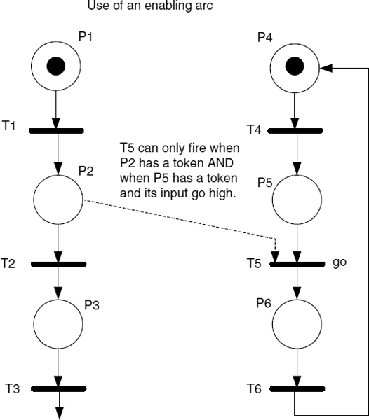
Figure 10.14 The enabling arc.

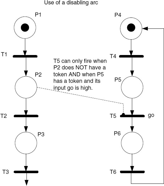
Figure 10.15 Disabling arc to avoid progression at a certain point in the Petri net.

Now consider the disabling arc in the example of Figure 10.15. In this example, the Petri net comprising P1 to P3 can stop the process in the other Petri net P4 to P6 if a token is in P2. This would be represented by the equation

T5 = /P2 · go · P5 · /P6.

Here, there must not be a token in P2, even if P5 has a token and input signal go = 1.

Now an example follows showing how these two ideas could be used in practice.

10.5 SYNCHRONIZATION OF TWO PETRI NETS USING ENABLING AND DISABLING ARCS

In the example of Figure 10.16, the sequence of flow is forced to follow a set sequence:

1. It is assumed that in this system the token will always arrive at P5 first, perhaps because of external circumstances.
2. The token in P5 cannot move on to P6 until the arrival of a token in P2.
3. The token cannot move on from P2 to P3 because T2 is disabled by the disabling arc from P5.
4. As soon as the input signal go = 1, the token in P5 can move to P6.
5. This removes the disablement of T2 and the token in P2 can move on to P3.

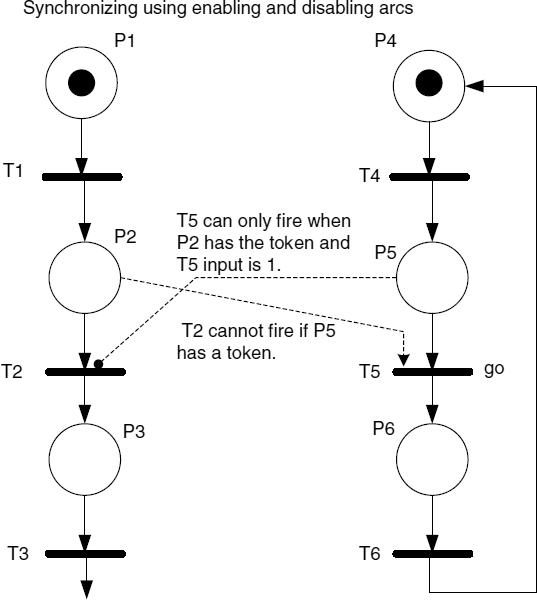
Figure 10.16 Provision of priority to a particular sequencing of two independent Petri nets.

This example illustrates the idea of how the enabling and disabling arcs can be used to check flow.

10.6 CONTROL OF A SHARED RESOURCE

Now consider the more practical example shown in Figure 10.17, which illustrates a system in which two computers, computer A and computer B, share a common resource (e.g. a printer) via a shared data bus. They are separated from the shared resource via tri-state buffers that are controlled by signals EA and EB via a Petri-net controller. Inputs to the Peri-net controller are ra and rb, which are sent by the respective computers. Computer A is to have priority over computer B.

There are a number of ways in which this problem could be resolved, but the most elegant is that shown in Figure 10.18. In this solution, two independent Petri nets have been used: one for processing the ra signal from computer A and the other from computer B.

If computer A accesses its ra signal before computer B accesses its rb signal, then the token in P1 will move to P2 and the disabling arc will disable T3 so that the arrival of a signal on rb will be blocked.

In due course, computer A will lower its ra signal and the token will move back to P1. If rb did arrive during the time that computer A had access to the shared resource, then the token in P3 will not move to P4 because T3 is disabled.

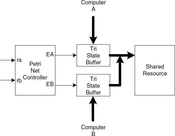
Figure 10.17 Shared resource controller.

Note that if computer Awants to access the shared resource again while computer B has access to it, raising its ra signal will cause the token in P4 to move back to P3 and the token in P1 will move to P2 as well. So, computer A has a priority over computer B.

Of course, if during the time that computer B has access to the shared resource there is no access by computer A, then, when computer B has finished its access, lowering of rb will cause the token to move back to P3.

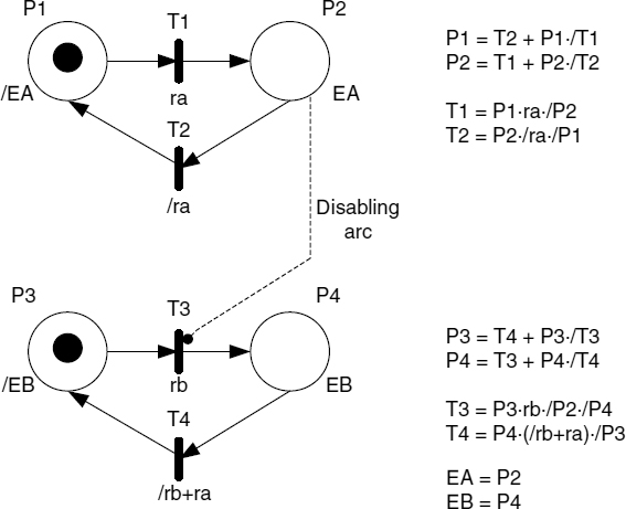
Figure 10.18 A solution to the shared resources problem.

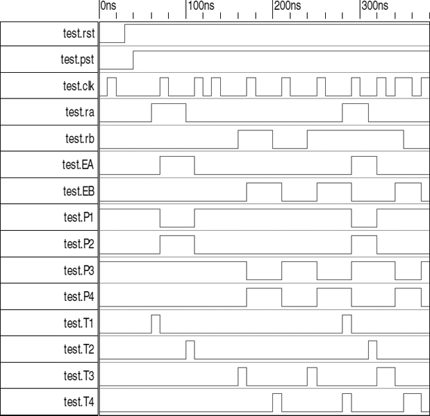
Figure 10.19 Simulation of the shared resource Petri net.

The equations for the Petri-net controller are given in Figure 10.18. In particular, note the equation for T3 with its disabling placeholder/P2 term. T3 can only fire if there is a token in P3 and rb is active high and there is not a token in P4 or P2.

At the start of the simulation (see Figure 10.19), P1 and P3 are active due to the initialization with rst and pst inputs (see Verilog HDL code in shared resource folder of Chapter 10 on the CDROM). Each input ra then rb is asserted in turn to simulate requests for access to the shared resource. At the seventh clock pulse the rb input has become active; then ra is active at the eighth clock pulse (priority request from computer A). This results in computer A gaining access to the shared resource from computer B. Computer A then completes its transaction and, since rb is still active, computer B regains access to the shared resource. In due course, rb returns to its low state and the Petri net returns the token in P4 to P3 to relinquish computer B access to the shared resource.

10.7 A SERIAL RECEIVER OF BINARY DATA

In Section 4.7, an asynchronous binary data receiver was developed using a state diagram implemented with D-type flip-flops, together with a shift register, a divide-by-11 counter and a data latch developed using the techniques in Appendix B.

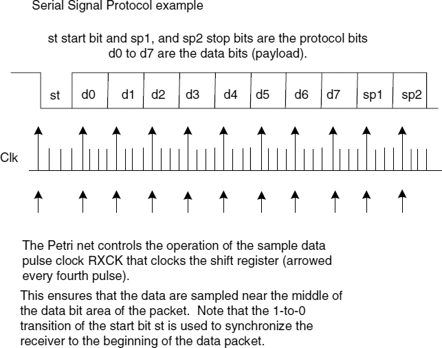
Figure 10.20 Arrangement of the data packet and protocol.

In this section, a similar design is described making use of a Petri-net controller. The design is described in detail, so it can be studied without reference to the one in Chapter 4.

An asynchronous serial receiver is to be developed using a Petri net to allow binary data to be received and converted into parallel data. The Petri net is a good way of implementing the serial receiver, since use can be made of the enabling arc and the design can be implemented using a single interconnected Petri net diagram.

As a reminder of the arrangement used in Chapter 4, the protocol and sample points are illustrated in Figure 10.20. The asynchronous serial protocol is to be one start bit (active low), followed by eight data bits, and two stop bits (11 bits in total). The incoming data need to be shifted into a shift register, and it is important to ensure that this is done when the incoming data have had time to settle. This can be achieved by using a clock that runs faster than the shift register clock so that the point in time that the shift register data is clocked into the shift register is around the middle of the available bit time interval.

In Figure 10.20, the bit time interval is around four clock periods, and at the second clock pulse into the data cell the data at the shift register input are to be clocked into the shift register (indicated by the arrowed clock pulse points). Thus, the shift register clock will be four times slower than the main state machine clock clk. This will be increased in this Petri net version.

Figure 10.21 illustrates a possible Petri-net-based block diagram for the system. In this system, a Petri-net controller is used to control the operation of the system, which consists of an 11-stage shift register with parallel outputs to a data latch. Note that the data into the data latch include only the data bits d0 to d7 (Q0 to Q7), not the protocol bits st, sp1, and sp2. The Divide-by-11 Counter (which could be either an asynchronous binary counter or a synchronous binary counter along the lines of those developed in Appendix B) is used to count the number of input data bits received and produces an output rxf indicating to the Petri net that the shift register is full. The shift register is clocked with the RXCK signal derived from the clk signal within the Petri-net controller.

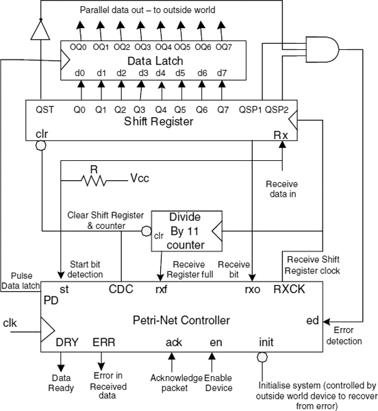
Figure 10.21 Block diagram for the asynchronous serial receiver system.

Should an error occur indicated by the ed signal, the error (ERR) output will be asserted high and the system will wait for a reinitialization from some external device ready for the next attempt at receiving a serial data packet. The control here would be via the external device using the serial receive system. The overall system is very similar to the one developed in Chapter 4.

The system is started by the start bit going low, as seen by the serial data in line. Figure 10.22 shows the Petri net diagram developed for the system. This consists of two Petri net diagrams connected by enabling arcs. The first one, comprising P1 to P5, is used to generate the shift register clock rxck. The second, and main, Petri net diagram controls the operation of the system. Both Petri nets are driven from the same clock clk.

Note the use of three enabling arcs. The first one, from PM2, is used to disable the first Petri net via its T1 firing transition until the main Petri net receives a start st data bit. The second enabling arc, from P5, is used to prevent the main Petri net from moving on to PM3 until the first Petri net has generated a shift-register clock pulse RXCK. Note, also, that an enabling arc is used to prevent T5 from firing until the main Petri net moves to PM3; otherwise, there is a potential race condition between T5 and TM2.

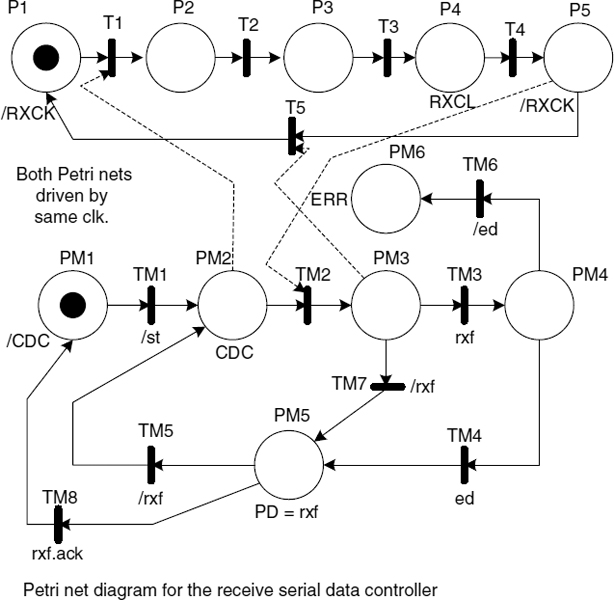
Figure 10.22 Petri net diagram for the asynchronous serial system.

Thus, the first Petri net can generate shift-register clock pulses at the correct time in the data packet. Note that there are five clock pulses between each RXCK in this realization, rather than the four as suggested in Figure 10.20. Thus, the system clock needs to be five times the required baud rate.

In the main Petri net, the placeholder PM3 and its two transitions TM3 and TM7 test for the shift-register full signal rxf. If low (shift register not full), then the main Petri net loops back to PM2.

Note that while rxf = 0, PM5 will not generate the PD signal (Mealy output). Also, TM5 can fire on rxf = 0. In due course a full data packet of 11 bits will be received. At this point, the main Petri net will move on to PM4 to check the ed signal. This signal should be high if st, sp1 and sp2 are received correctly. This being the case, the main Petri net will move on to PM5, where it will issue a PD signal (since rxf = 1 now) to latch the received data into the data latch ready to be collected by the outside world.

The main Petri net will wait for an ack signal (since rxf = 1 now) from the outside world (indicating that the data have been read) before returning the token to the PM1 placeholder and resetting the shift register and 11-bit counter.

In this Petri net, use has been made of enabling arcs to synchronize the two Petri nets, and a Mealy output for signal PD allows a common loop to be used under different conditions.

10.7.1 Equations for the First Petri Net

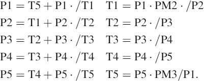
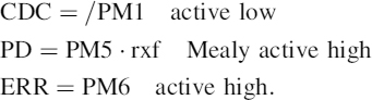
10.7.2 Output

RXCK = P4

10.7.3 Equations for the Main Petri Net

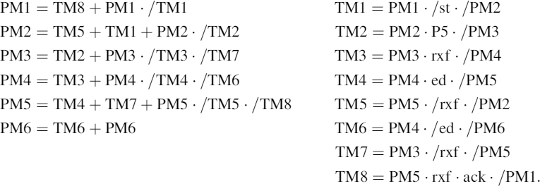
10.7.4 Outputs

The simulation of the Petri net for the receiver is illustrated in Figure 10.23. In this simulation, a test-bench module has been developed so that all paths through the Petri net can be checked. This has required manipulation of the rxf, ack, and ed signals that would normally be controlled by the external controller. A study of the waveforms in Figure 10.23 shows the test paths.

Essentially, the simulation shows how the enabling arcs control the sequence of both the shift clock generation produced by P1 to P5, and the main Petri net PM1 to PM6.

Further study of the waveforms reveals the sequence between RXCK pulses, as shown in Figure 10.24. This indicates that, during the serial data receiving phase, a shift register pulse occurs every seven FSM clock pulses. Therefore, for a baud rate of 1 × 10⁶ bits per second, an FSM clock of 7 MHz would be required.

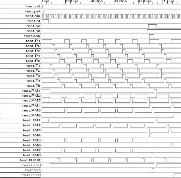
Figure 10.23 Simulation of the Petri net.

The action of the enabling arcs can be clearly seen in Figure 10.23. The simulation ends with an error signal forcing the Petri net into PM6.

The complete Verilog HDL listing can be found on the CDROM in the Chapter 10 folder.

To develop the entire system, the shift register, divide-by-11 counter, the logic AND gate, and data latch also need to be defined and connected together.

10.7.5 The Shift Register

This is an 11-bit device. See Figure B.12a and b in Appendix B for details.

10.7.6 Equations for the Shift Register

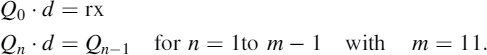
For a general shift register of m stages (number of D-type flip-flops)

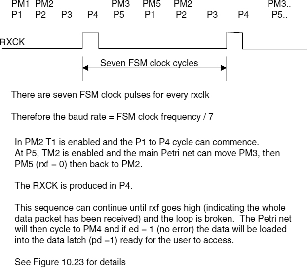
Figure 10.24 Details of Petri net sequence during data receive phase.

for all remaining flip flops where n = 1 to n = m − 1, where m is the number of flip-flops in the shift register.

From this, the equations for the 11-stage shift register are

There is no need to gate the shift-register clock rxck, since it is controlled by the Petri-net controller.

10.7.7 The Divide-by-11 Counter

This can be either a common asynchronous binary counter (ripple through) or a synchronous type. See Appendix B, Section B.9.2 and Figure B.13a and b, for details.

10.7.8 The Data Latch

This is a standard design parallel data latch with eight D-type flip flops each having a data input and data output and all clocked by the pulse data latch signal PD.

Parity detection logic could be added and would follow along the same lines as that used in Chapter 4.

10.8 SUMMARY

The use of Petri nets can provide a means by which parallel control can be realized in hardware. This chapter has explored this area and shown how such systems could be developed and implemented using an HDL. The use of enabling/disabling arcs can help to synchronize parallel Petri net activities.

REFERENCE

1. Fernandes JM, Adamski M, Proeca AJ. VHDL generation from hierarchical Petri net specifications of parallel controllers. IEE Proc Comput Digital Technol 1997; 144(2): 127–135.

All Petri Net Equation generations are reproduced from ‘VHDL generation from hierarchical Petri net specifications of parallel controllers’ by JM Fernandes, M Adamski and A J Proenca, (IEE Proceedings-Computers and Digital Techniques, Vol.144, No.2 March 2007) with permission from IET.