
The term architecture is used in this chapter to mean the process structure of a concurrent program together with the way in which the elements of the program interact. For example, the client–server architecture of Chapter 10 is a structure consisting of one or more client processes interacting with a single server process. The interaction is bi-directional consisting of a request from a client to the server and a reply from the server to the client. This organization is at the heart of many distributed computing applications. The client–server architecture can be described independently of the detailed operation of client and server processes. We do not need to consider the service provided by the server or indeed the use the client makes of the result obtained from requesting the service. In describing the concurrent architecture of a program, we can ignore many of the details concerned with the application that the program is designed to implement. The advantage of studying architecture is that we can examine concurrent program structures that can be used in many different situations and applications. In the following, we look at some architectures that commonly occur in concurrent programs.
A filter is a process that receives a stream of input values, performs some computation on these values and sends a stream of results as its output. In general, a filter can have more than one input stream and produce results on more than one output stream. Filters can easily be combined into larger computations by connecting the output stream from one filter to the input stream of another. Where filters have more than one input and output, they can be arranged into networks with complex topologies. In this section, we restrict the discussion to filters that have a single input and a single output. Such filters can be combined into pipeline networks. Many of the user-level commands in the UNIX operating system are filter processes, for example the text formatting programs tbl, eqn and troff. In UNIX, filter processes can be combined using pipes. A UNIX pipe is essentially a bounded buffer that buffers bytes of data output by one filter until they are input to the next filter. We will see in the following that the pipes that interconnect filters do not always need to include buffering.
To illustrate the use of filter pipelines, we develop a program with this architecture that computes prime numbers. The program is a concurrent implementation of a classic algorithm known as the Primes Sieve of Eratosthenes, after the Greek mathematician who developed it. The algorithm to determine all the primes between 2 and n proceeds as follows. First, write down a list of all the numbers between 2 and n:
2 3 4 5 6 7 ... n
Then, starting with the first uncrossed-out number in the list, 2, cross out each number in the list which is a multiple of 2:
2 3

Now move to the next uncrossed-out number, 3, and repeat the above by crossing out multiples of 3. Repeat the procedure until the end of the list is reached. When finished, all the uncrossed-out numbers are primes. The primes form a sieve which prevents their multiples falling through into the final list.
The concurrent version of the primes sieve algorithm operates by generating a stream of numbers. The multiples are removed by filter processes. The outline architecture of the program is depicted in Figure 11.1. It is essentially a process structure diagram from which we have omitted the details of action and process labels.
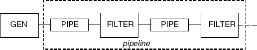
The diagram describes the high-level structure of the program. The process GEN generates the stream of numbers from which multiples are filtered by the FILTER processes. To fully capture the architecture of the program, we must also consider how the application-specific processes interact. Interaction between these elements in the example is described by the PIPE processes. In the terminology of Software Architecture, these processes are termed connectors. Connectors encapsulate the interaction between the components of the architecture. Connectors and components are both modeled as processes. The distinction with respect to modeling is thus essentially methodological. We model the pipe connectors in the example as one-slot buffers as shown below:
const MAX = 9
     range NUM = 2..MAX
     set S = {[NUM],eos}
     PIPE = (put[x:S]->get[x]->PIPE).
The PIPE process buffers elements from the set S which consist of the numbers 2..MAX and the label eos, which is used to signal the end of a stream of numbers. This end of stream signal is required to correctly terminate the program.
To simplify modeling of the GEN and FILTER processes, we introduce an additional FSP construct – the conditional process. The construct can be used in the definition of both primitive and composite processes.
Note
The process if B then P else Q behaves as the process P if the condition B is true otherwise it behaves as Q. If the else Q is omitted and B is false, then the process behaves as STOP.
The definition of GEN using the conditional process construct is given below:
GEN       = GEN[2],
     GEN[x:NUM] = (out.put[x] ->
                    if x<MAX then
                    GEN[x+1]
                    else
                    (out.put.eos->end->GEN)
                  ).
The GEN process outputs the numbers 2 to MAX, followed by the signal eos. The action end is used to synchronize termination of the GEN process and the filters. After end occurs, the model re-initializes rather than terminates. This is done so that, if deadlock is detected during analysis, it will be an error and not because of correct termination. The FILTER process records the first value it gets and subsequently filters out multiples of that value from the numbers it receives and forwards to the next filter in the pipeline.
FILTER = (in.get[p:NUM]->prime[p]->FILTER[p]
              |in.get.eos->ENDFILTER
              ),
     FILTER[p:NUM] = (in.get[x:NUM] ->
                       if x%p!=0 then
                         (out.put[x]->FILTER[p])
                       else
                         FILTER[p]
                     |in.get.eos->ENDFILTER
                     ),
     ENDFILTER     = (out.put.eos->end->FILTER).
The composite process that conforms to the structure given in Figure 11.1 can now be defined as:
||PRIMES(N=4) =
        ( gen:GEN
        ||pipe[0..N-1]:PIPE
        ||filter[0..N-1]:FILTER
        )/{ pipe[0]/gen.out,
            pipe[i:0..N-1]/filter[i].in,
            pipe[i:1..N-1]/filter[i-1].out,
            end/{filter[0..N-1].end,gen.end}
          }@{filter[0..N-1].prime,end}.
Safety analysis of this model detects no deadlocks or errors. The minimized LTS for the model is depicted in Figure 11.2. This confirms that the model computes the primes between 2 and 9 and that the program terminates correctly.
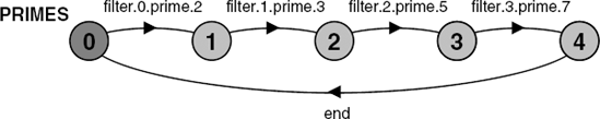
In fact, the concurrent version of the primes sieve algorithm does not ensure that all the primes between 2 and MAX are computed: it computes the first N primes where N is the number of filters in the pipeline. This can easily be confirmed by changing MAX to 11 and re-computing the minimized LTS, which is the same as Figure 11.2. To compute all the primes in the range 2 to 11, five filters are required.
We have modeled the filter pipeline using single-slot buffers as the pipes connecting filters. Would the behavior of the overall program change if we used unbuffered pipes? This question can easily be answered by constructing a model in which the PIPE processes are omitted and instead, filters communicate directly by shared actions. This model is listed below. The action pipe[i] relabels the out.put action of filter[i-1] and the in.get action of filter[i].
||PRIMESUNBUF(N=4) =
       (gen:GEN || filter[0..N-1]:FILTER)
         /{ pipe[0]/gen.out.put,
           pipe[i:0..N-1]/filter[i].in.get,
           pipe[i:1..N-1]/filter[i-1].out.put,
           end/{filter[0..N-1].end,gen.end}
         }@{filter[0..N-1].prime,end}.
The minimized LTS for the above model is depicted in Figure 11.3.
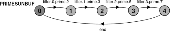
The reader can see that the LTS of Figure 11.3 is identical to that of Figure 11.2. The behavior of the program with respect to generating primes and termination has not changed with the removal of buffers. Roscoe (1998) describes a program as being buffer tolerant if its required behavior does not change with the introduction of buffers. We have shown here that the primes sieve program is buffer tolerant to the introduction of a single buffer in each pipe. Buffer tolerance is an important property in the situation where we wish to distribute a concurrent program and, for example, locate filters on different machines. In this situation, buffering may be unavoidable if introduced by the communication system.
We showed above that the primes sieve program is tolerant to the introduction of a single buffer in each pipe. The usual problem of state space explosion arises if we try to analyze a model with more buffers. To overcome this problem, we can abstract from the detailed operation of the primes sieve program. Instead of modeling how primes are computed, we concentrate on how the components of the program interact, independently of the data values that they process. The abstract versions of components can be generated mechanically by relabeling the range of values NUM to be a single value. This is exactly the same technique that we used in section 10.2.2 to generate an abstract model of an asynchronous message port. The abstract versions of GEN, FILTER and PIPE are listed below.
||AGEN    = GEN/{out.put/out.put[NUM]}.

     ||AFILTER = FILTER/{out.put/out.put[NUM],
                         in.get /in.get.[NUM],
                         prime /prime[NUM]
                        }.

     ||APIPE   = PIPE/{put/put[NUM],get/get[NUM]}.
The LTS for the abstract version of a filter process is shown in Figure 11.4. In the detailed version of the filter, the decision to output a value depends on the computation as to whether the value is a multiple of the filter's prime. In the abstract version, this computation has been abstracted to the non-deterministic choice as to whether, in state (4), after an in.get action, the LTS moves to state (5) and does an out.put action or remains in state (4). This is a good example of how nondeterministic choice is used to abstract from computation. We could, of course, have written the abstract versions of the elements of the primes sieve program directly, rather than writing detailed versions and abstracting mechanically as we have done here. In fact, since FSP, as a design choice, has extremely limited facilities for describing and manipulating data, for complex programs abstraction is usually the best way to proceed.
To analyze the primes sieve program with multi-slot pipes, we can use a pipeline of APIPE processes defined recursively as follows:
||MPIPE(B=4) =
       if B==1 then
         APIPE
       else
         (APIPE/{mid/get} || MPIPE(B-1)/{mid/put})
       @{put,get}.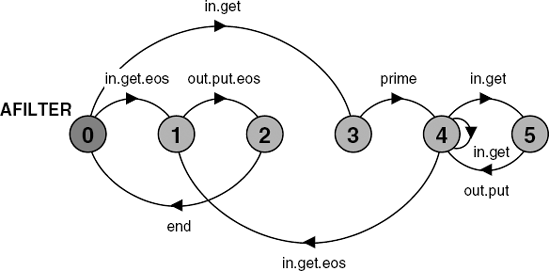
The abstract model for the primes program, with exactly the architecture of Figure 11.1, can now be defined as:
||APRIMES(N=4,B=3) =
        (gen:AGEN || PRIMEP(N)
        || pipe[0..N-1]:MPIPE(B)
        || filter[0..N-1]:AFILTER)
        /{ pipe[0]/gen.out,
           pipe[i:0..N-1]/filter[i].in,
           pipe[i:1..N-1]/filter[i-1].out,
           end/{filter[0..N-1].end,gen.end}
         }.
where PRIMEP is a safety property which we define in the following discussion.
We refer to the properties that we can assert for the abstract model of the primes sieve program as architectural properties since they are concerned with the concurrent architecture of the program – structure and interaction – rather than its detailed operation. The general properties we wish to assert at this level are absence of deadlock and eventual termination (absence of livelock). Eventual termination is checked by the progress property END, which asserts that, in all executions of the program, the terminating action end must always occur.
progress END = {end}The property specific to the application is that the prime from filter[0] should be produced before the prime from filter[1] and so on. The following safety property asserts this:
propertyPRIMEP(N=4) = PRIMEP[0], PRIMEP[i:0..N]= (when(i<N) filter[i].prime->PRIMEP[i+1] |end -> PRIMEP ).
The property does not assert that all the filters must produce primes before end occurs since the model can no longer determine that there are four primes between 2 and 9.
Analysis of APRIME using LTSA determines that there are no deadlocks, safety violations or progress violations for four filters and three slot pipes. The reader should verify that the safety and progress properties hold for other combinations of filters and buffering. When building this model, it is important that the LTSA option Minimize during composition is set, otherwise the minimized models for the abstracted elements are not built and consequently, the reduction in state space is not realized.
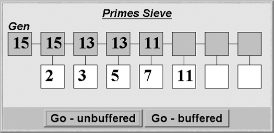
Figure 11.5 is a screen shot of the Primes Sieve applet display. The implementation supports both a buffered and unbuffered implementation of the pipe connector. The figure depicts a run using unbuffered pipes. The box in the top left hand of the display depicts the latest number generated by the thread that implements GEN. The rest of the boxes, at the top, display the latest number received by a filter. The boxes below display the prime used by that filter to remove multiples.
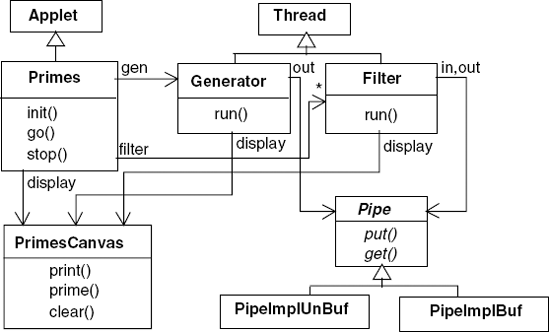
The implementation follows in a straightforward way from the model developed in the previous section. The number generator and filter processes are implemented as threads. As mentioned above, we have provided two implementations for the pipe connector. The classes involved in the program and their inter-relationships are depicted in the class diagram of Figure 11.6. The display is handled by a single class, PrimesCanvas. The methods provided by this class, together with a description of their functions, are listed in Program 11.1.
The code for the Generator and Filter threads is listed in Programs 11.2 and 11.3. The implementation of these threads corresponds closely to the detailed models for GEN and FILTER developed in the previous section. Additional code has been added only to display the values generated and processed. To simplify the display and the pipe implementations, the end-of-stream signal is an integer value that does not occur in the set of generated numbers. The obvious values to use are 0, 1, −1 or MAX+1. In the applet class, Primes.EOS is defined to be −1.
Instead of implementing buffered and unbuffered pipes from scratch, we have reused classes developed in earlier chapters. The synchronous message-passing class, Channel, from Chapter 10 is used to implement an unbuffered pipe and the bounded buffer class, BufferImpl, from Chapter 5 is used to implement buffered pipes. The Pipe interface and its implementations are listed in Program 11.4.
Example 11.1. PrimesCanvas class.
classPrimesCanvasextendsCanvas {// displayvalin an upper box numberedindex// boxes are numbered from the leftsynchronizedvoid print(int index, int val){...}// display,valin a lower box numberedindex// the lower box indexed by 0 is not displayedsynchronizedvoid prime(int index, int val){...}// clear all boxessynchronizedvoid clear(){...} }
Example 11.2. Generator class.
classGeneratorextendsThread {privatePrimesCanvas display;privatePipe<Integer> out;staticint MAX = 50; Generator(Pipe<Integer> c, PrimesCanvas d) {out=c; display = d;}publicvoid run() {try{for(int i=2;i<=MAX;++i) { display.print(0,i); out.put(i); sleep(500); } display.print(0,Primes.EOS); out.put(Primes.EOS); }catch(InterruptedException e){} } }
Example 11.3. Filter class.
classFilterextendsThread {privatePrimesCanvas display;privatePipe<Integer> in,out;privateint index; Filter(Pipe<Integer> i, Pipe<Integer> o, int id, PrimesCanvas d) {in = i; out=o;display = d; index = id;}publicvoid run() { int i,p;try{ p = in.get(); display.prime(index,p);if(p==Primes.EOS && out!=null) { out.put(p);return; }while(true) { i= in.get(); display.print(index,i); sleep(1000);if(i==Primes.EOS) {if(out!=null) out.put(i);break; }elseif (i%p!=0 && out!=null) out.put(i); } }catch(InterruptedException e){} } }
The structure of a generator thread and N filter threads connected by pipes is constructed by the go() method of the Primes applet class. The code is listed below:
Example 11.4. Pipe, PipeImplUnBuf and PipeImplBuf classes.
publicinterface Pipe<T> {publicvoid put(T o)throwsInterruptedException;// put object into bufferpublicT get()throwsInterruptedException;// get object from buffer}// Unbuffered pipe implementationpublic classPipeImplUnBuf<T>implementsPipe<T> { Channel<T> chan =newChannel<T>();publicvoid put(T o)throwsInterruptedException { chan.send(o); }publicT get() throws InterruptedException {returnchan.receive(); } }// Buffered pipe implementationpublic classPipeImplBuf<T> implements Pipe<T> { Buffer<T> buf =newBufferImpl<T>(10);publicvoid put(T o)throwsInterruptedException { buf.put(o); }publicT get()throwsInterruptedException {returnbuf.get(); } }
privatevoid go(boolean buffered) { display.clear();//create channelsArrayList<Pipe<Integer> pipes =newArrayList<Pipe<Integer>();
for(int i=0; i<N; ++i)if(buffered) pipes.add(new PipeImplBuf<Integer>());elsepipes.add(new PipeImplUnBuf<Integer>());//create threadsgen =newGenerator(pipes.get(0),display);for(int i=0; i<N; ++i) filter[i] =newFilter(pipes.get(i), i<N-1?pipes.get(i+1):null,i+1,display); gen.start();for(int i=0; i<N; ++i) filter[i].start(); }
We saw from modeling the primes sieve program that it computed the correct result, whether or not the pipes connecting filter processes were buffered. In line with the model, the implementation also works correctly with and without buffers. Why then should we ever use buffering in this sort of architecture when the logical behavior is independent of buffering? The answer is concerned with the execution efficiency of the program.
When a process or thread suspends itself and another is scheduled, the operating system performs a context switch which, as discussed in Chapter 3, involves saving the registers of the suspended process and loading the registers for the newly scheduled process. Context switching consumes CPU cycles and, although the time for a thread switch is much less than that for an operating system process, it is nevertheless an overhead. A concurrent program runs faster if we can reduce the amount of context switching. With no buffering, the generator and filter threads are suspended every time they produce an item until that item is consumed by the next thread in the pipeline. With buffers, a thread can run until the buffer is full. Consequently, in a filter pipeline, buffering can reduce the amount of context switching. In our implementation, this benefit is not actually realized since we have introduced delays for display purposes. However, it is generally the case that a pipeline architecture performs better with buffered pipes.
If filters are located on physically distributed processors, buffering has an additional advantage. When a message is sent over a communication link, there is a fixed processing and transmission overhead that is independent of message size. Consequently, when transmitting a lot of data, it is better to transmit a few large messages rather than many small messages. With buffering in the filter pipeline, it is easy to arrange that a sequence of items be sent in the same message.
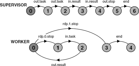
Supervisor–Worker is a concurrent architecture that can be used to speed up the execution of some computational problems by exploiting parallel execution on multiple processors. The architecture applies when a computational problem can be split up into a number of independent sub-problems. These independent sub-problems are referred to as tasks in the following discussion. The process architecture of a Supervisor–Worker program is depicted in Figure 11.7.
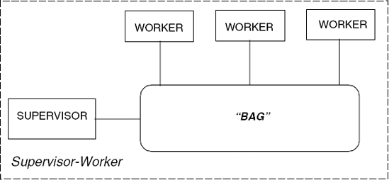
Supervisor and worker processes interact by a connector that we refer to, for the moment, as a "bag". The supervisor process is responsible for generating an initial set of tasks and placing them in the bag. Additionally, the supervisor collects results from the bag and determines when the computation has finished. Each worker repetitively takes a task from the bag, computes the result for that task, and places the result in the bag. This process is repeated until the supervisor signals that the computation has finished. The architecture can be used to parallelize divide-and-conquer problems since workers can put new tasks into the bag as well as results. Another way of thinking of this is that the result computed by a worker can be a new set of tasks. Thus, in a divide-and-conquer computation, the supervisor places an initial task in the bag and this is split into two further problems by a worker and so on. We can use any number of worker processes in the Supervisor–Worker architecture. Usually, it is best to have one worker process per physical processor. First, we examine an interaction mechanism suitable for implementing the bag connector.
Linda is the collective name given by Carriero and Gelernter (1989a) to a set of primitive operations used to access a data structure called a tuple space. A tuple space is a shared associative memory consisting of a collection of tagged data records called tuples. Each data tuple in a tuple space has the form:
("tag", value1,..., valuen)
The tag is a literal string used to distinguish between tuples representing different classes of data. valuei are zero or more data values: integers, floats and so on.
There are three basic Linda operations for manipulating data tuples: out, in and rd. A process deposits a tuple in a tuple space using:
out ("tag", expr1,..., exprn)
Execution of out completes when the expressions have been evaluated and the resulting tuple has been deposited in the tuple space. The operation is similar to an asynchronous message send except that the tuple is stored in an unordered tuple space rather than appended to the queue associated with a specific port. A process removes a tuple from the tuple space by executing:
in ("tag", field1,..., fieldn)
Each field i is either an expression or a formal parameter of the form ?var where var is a local variable in the executing process. The arguments to in are called a template; the process executing in blocks until the tuple space contains a tuple that matches the template and then removes it. A template matches a data tuple in the following circumstances: the tags are identical, the template and tuple have the same number of fields, the expressions in the template are equal to the corresponding values in the tuple, and the variables in the template have the same type as the corresponding values in the tuple. When the matching tuple is removed from the tuple space, the formal parameters in the template are assigned the corresponding values from the tuple. The in operation is similar to a message receive operation with the tag and values in the template serving to identify the port.
The third basic operation is rd, which functions in exactly the same way as in except that the tuple matching the template is not removed from the tuple space. The operation is used to examine the contents of a tuple space without modifying it. Linda also provides non-blocking versions of in and rd called inp and rdp whichreturntrueif amatchingtupleis found and return false otherwise.
Linda has a sixth operation called eval that creates an active or process tuple. The eval operation is similar to an out except that one of the arguments is a procedure that operates on the other arguments. A process is created to evaluate the procedure and the process tuple becomes a passive data tuple when the procedure terminates. This eval operation is not necessary when a system has some other mechanism for creating new processes. It is not used in the following examples.
Our modeling approach requires that we construct finite state models. Consequently, we must model a tuple space with a finite set of tuple values. In addition, since a tuple space can contain more than one tuple with the same value, we must fix the numberof copies of each value that are allowed. We define this number to be the constant N and the allowed values to be the set Tuples.
constN = ...setTuples = {...}
The precise definition of N and Tuples depends on the context in which we use the tuple space model. Each tuple value is modeled by an FSP label of the form tag.val1... valn. We define a process to manage each tuple value and the tuple space is then modeled by the parallel composition of these processes:
constFalse = 0constTrue = 1rangeBool = False..True TUPLE(T='any) = TUPLE[0], TUPLE[i:0..N] = (out[T] -> TUPLE[i+1] |when(i>0) in[T] -> TUPLE[i-1] |when(i>0) inp[True][T] -> TUPLE[i-1] |when(i==0)inp[False][T] -> TUPLE[i] |when(i>0) rd[T] -> TUPLE[i] |rdp[i>0][T] -> TUPLE[i] ). ||TUPLESPACE =forall[t:Tuples] TUPLE(t).
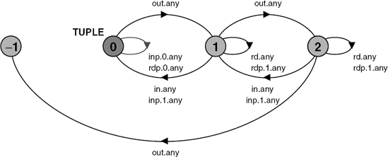
The LTS for TUPLE value any with N=2 is depicted in Figure 11.8. Exceeding the capacity by performing more than two out operations leads to an ERROR.
An example of a conditional operation on the tuple space would be:
inp[b:Bool][t:Tuples]
The value of the local variable t is only valid when b is true. Each TUPLE process has in its alphabet the operations on one specific tuple value. The alphabet of TUPLESPACE is defined by the set TupleAlpha:
set TupleAlpha
  = {{in,out,rd,rdp[Bool],inp[Bool]}.Tuples}
A process that shares access to the tuple space must include all the actions of this set in its alphabet.
Linda tuple space can be distributed over many processors connected by a network. However, for demonstration purposes we describe a simple centralized implementation that allows matching of templates only on the tag field of a tuple. The interface to our Java implementation of a tuple space is listed in Program 11.5.
Example 11.5. TupleSpace interface.
public interfaceTupleSpace {// deposits data in tuple spacepublicvoid out (String tag, Object data);// extracts object with tag from tuple space, blocks if not availablepublicObject in (String tag)throwsInterruptedException;// reads object with tag from tuple space, blocks if not availablepublicObject rd (String tag)
throwsInterruptedException;// extracts object if available, return null if not availablepublicObject inp (String tag);// reads object if available, return null if not availablepublicObject rdp (String tag); }
We use a hash table of vectors to implement the tuple space (Program 11.6). Although the tuple space is defined to be unordered, for simplicity, we have chosen to store the tuples under a particular tag in FIFO order. New tuples are appended to the end of a vector for a tag and removed from its head. For simplicity, a naive synchronization scheme is used which wakes up all threads whenever a new tuple is added. A more efficient scheme would wake up only those threads waiting for a tuple with the same tag as the new tuple.
We model a simple Supervisor–Worker system in which the supervisor initially outputs a set of tasks to the tuple space and then collects results. Each worker repetitively gets a task and computes the result. The algorithms for the supervisor and each worker process are sketched below:
Supervisor::
     forall tasks: out("task",...)
     forall results: in("result",...)
     out("stop")
   Worker::
     while not rdp("stop") do
        in("task",...)
        compute result
        out("result",...)
To terminate the program, the supervisor outputs a tuple with the tag "stop" when it has collected all the results it requires. Workers run until they read this tuple. The set of tuple values and the maximum number of copies of each value are defined for the model as:
constN = 2setTuples = {task,result,stop}
Example 11.6. TupleSpaceImpl class.
classTupleSpaceImplimplementsTupleSpace {privateHashtable tuples =newHashtable();public synchronizedvoid out(String tag,Object data){ Vector v = (Vector) tuples.get(tag);if(v == null) { v = new Vector(); tuples.put(tag,v); } v.addElement(data); notifyAll(); }privateObjectget(String tag, boolean remove) { Vector v = (Vector) tuples.get(tag);if(v == null)returnnull;if(v.size() == 0)returnnull; Object o = v.firstElement();if(remove) v.removeElementAt(0);returno; }public synchronizedObject in (String tag)throwsInterruptedException { Object o;while((o = get(tag,true)) == null) wait();returno; }publicObject rd (String tag)throwsInterruptedException { Object o;while((o = get(tag,false)) == null) wait();returno; }public synchronizedObject inp (String tag) { return get(tag,true); }public synchronizedObject rdp (String tag) {returnget(tag,false); } }
The supervisor outputs N tasks to the tuple space, collects N results and then outputs the "stop" tuple and terminates.
SUPERVISOR   = TASK[1],
     TASK[i:1..N] =
       (out.task  ->
          if i<N then TASK[i+1] else RESULT[1]),
     RESULT[i:1..N] =
       (in.result ->
          if i<N then RESULT[i+1] else FINISH),
     FINISH =
       (out.stop  -> end -> STOP) + TupleAlpha.
The worker checks for the "stop" tuple before getting a task and outputting the result. The worker terminates when it reads "stop" successfully.
WORKER =
       (rdp[b:Bool].stop->
         if (!b) then
           (in.task -> out.result -> WORKER)
         else
           (end -> STOP)
       )+TupleAlpha.
The LTS for both SUPERVISOR and WORKER with N=2 is depicted in Figure 11.9.
In the primes sieve example, we arranged that the behavior was cyclic to avoid detecting a deadlock in the case of correct termination. An alternative way of avoiding this situation is to provide a process that can still engage in actions after the end action has occurred. We use this technique here and define an ATEND process that engages in the action ended after the correct termination action end occurs.
ATEND   = (end->ENDED),
     ENDED = (ended->ENDED).
A Supervisor–Worker model with two workers called redWork and blueWork, which conforms to the architecture of Figure 11.7, can now be defined by:
||SUPERVISOR_WORKER
         = ( supervisor:SUPERVISOR
           || {redWork,blueWork}:WORKER
           || {supervisor,redWork,blueWork}::TUPLESPACE
           || ATEND
)/{end/{supervisor,redWork,blueWork}.end}.Safety analysis of this model using LTSA reveals the following deadlock:
Trace to DEADLOCK:
         supervisor.out.task
         supervisor.out.task
         redWork.rdp.0.stop            – rdp returns false
         redWork.in.task
         redWork.out.result
         supervisor.in.result
         redWork.rdp.0.stop            – rdp returns false
         redWork.in.task
         redWork.out.result
         supervisor.in.result
         redWork.rdp.0.stop            – rdp returns false
         supervisor.out.stop
         blueWork.rdp.1.stop           – rdp returns true
This trace is for an execution in which the red worker computes the results for the two tasks put into tuple space by the supervisor. This is quite legitimate behavior for a real system since workers can run at different speeds and take different amounts of time to start. The deadlock occurs because the supervisor only outputs the "stop" tuple after the red worker attempts to read it. When the red worker tries to read, the "stop" tuple has not yet been put into the tuple space and, consequently, the worker does not terminate but blocks waiting for another task. Since the supervisor has finished, no more tuples will be put into the tuple space and consequently, the worker will never terminate.
This deadlock, which can be repeated for different numbers of tasks and workers, indicates that the termination scheme we have adopted is incorrect. Although the supervisor completes the computation, workers may not terminate. It relies on a worker being able to input tuples until it reads the "stop" tuple. As the model demonstrates, this may not happen. This would be a difficult error to observe in an implementation since the program would produce the correct computational result. However, after an execution, worker processes would be blocked and consequently retain execution resources such as memory and system resources such as control blocks. Only after a number of executions might the user observe a system crash due to many hung processes. Nevertheless, this technique of using a "stop" tuple appears in an example Linda program in a standard textbook on concurrent programming!
A simple way of implementing termination correctly would be to make a worker wait for either inputting a "task" tuple or reading a "stop" tuple. Unfortunately, while this is easy to model, it cannot easily be implemented since Linda does not have an equivalent to the selective receive described in Chapter 10. Instead, we adopt a scheme in which the supervisor outputs a "task" tuple with a special stop value. When a worker inputs this value, it outputs it again and then terminates. Because a worker outputs the stop task before terminating, each worker will eventually input it and terminate. This termination technique appears in algorithms published by the designers of Linda (Carriero and Gelernter, 1989b). The revised algorithms for supervisor and worker are sketched below:
Supervisor:: forall tasks:-out("task",...) forall results:-in("result",...)out("task",stop)Worker:: while true doin("task",...) if value isstopthenout("task",stop); exit compute resultout("result",...)
The tuple definitions and models for supervisor and worker now become:
set Tuples  = {task,task.stop,result}

SUPERVISOR   = TASK[1],
TASK[i:1..N] =
out.task ->ifi<NthenTASK[i+1]elseRESULT[1]), RESULT[i:1..N] = (in.result ->ifi<NthenRESULT[i+1]elseFINISH), FINISH = (out.task.stop -> end -> STOP) + TupleAlpha. WORKER = (in.task -> out.result -> WORKER |in.task.stop -> out.task.stop -> end ->STOP ) + TupleAlpha.
The revised model does not deadlock and satisfies the progress property:
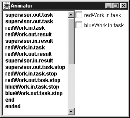
progress END = {ended}A sample trace from this model, which again has the red worker computing both tasks, is shown in Figure 11.10.
In the first section of this chapter, the primes sieve application was modeled in some detail. We then abstracted from the application to investigate the concurrent properties of the Filter Pipeline architecture. In this section, we have modeled the Supervisor–Worker architecture directly without reference to an application. We were able to discover a problem with termination and provide a general solution that can be used in any application implemented within the framework of the architecture.
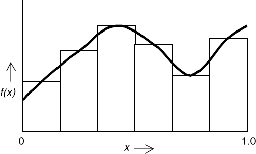
To illustrate the implementation and operation of Supervisor–Worker architectures, we develop a program that computes an approximate value of the area under a curve using the rectangle method. More precisely, the program computes an approximate value for the integral:

The rectangle method involves summing the areas of small rectangles that nearly fit under the curve as shown in Figure 11.11.
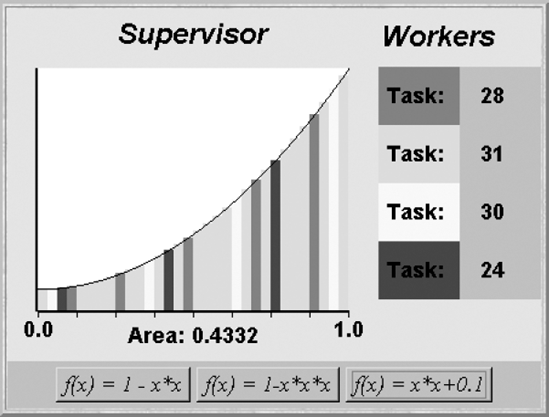
In the Supervisor–Worker implementation, the supervisor determines how many rectangles to compute and hands the task of computing the area of the rectangles to the workers. The demonstration program has four worker threads each with a different color attribute. When the supervisor inputs a result, it displays the rectangle corresponding to that result with the color of the worker. The display of a completed computation is depicted in Figure 11.12.
Each worker is made to run at a different speed by performing a delay before outputting the result to the tuple space. The value of this delay is chosen at random when the worker is created. Consequently, each run behaves differently. The display of Figure 11.12 depicts a run in which some workers compute more results than others. During a run, the number of the task that each worker thread is currently computing is displayed. The last task that the worker completed is displayed at the end of a run. The class diagram for the demonstration program is shown in Figure 11.13.
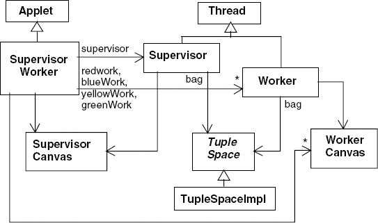
The displays for the supervisor and worker threads are handled, respectively, by the classes SupervisorCanvas and WorkerCanvas. The methods provided by these classes, together with a description of what they do, are listed in Program 11.7. The interface for the function f(x) together with three implementations are also included in Program 11.7.
Example 11.7. SupervisorCanvas, WorkerCanvas and Function classes.
classSupervisorCanvasextendsCanvas {// display rectangle sliceiwith colorc,addato area fieldsynchronizedvoid setSlice( int i,double a,Color c) {...}// reset display to clear rectangle slices and draw curve forfsynchronizedvoid reset(Function f) {...} }classWorkerCanvasextendsPanel {// display current task numbervalsynchronizedvoid setTask(int val) {...} }interfaceFunction { double fn(double x); }classOneMinusXsquaredimplementsFunction {publicdouble fn (double x) {return1-x*x;} }classOneMinusXcubed implements Function {publicdouble fn (double x) {return1-x*x*x;} }classXsquaredPlusPoint1 implements Function { public double fn (double x) {returnx*x+0.1;} }
A task that is output to the tuple space by the supervisor thread is represented by a single integer value. This value identifies the rectangle for which the worker computes the area. A result requires a more complex data structure since, for display purposes, the result includes the rectangle number and the worker color attribute in addition to the computed area of the rectangle. The definition of the Result and the Supervisor classes is listed in Program 11.8.
The supervisor thread is a direct translation from the model. It outputs the set of rectangle tasks to the tuple space and then collects the results. Stop is encoded as a "task" tuple with the value −1, which falls outside the range of rectangle identifiers. The Worker thread class is listed in Program 11.9.
Example 11.8. Result and Supervisor classes.
classResult { int task; Color worker; double area; Result(int s, double a, Color c) {task =s; worker=c; area=a;} }classSupervisorextendsThread { SupervisorCanvas display; TupleSpace bag; Integer stop =newInteger(-1); Supervisor(SupervisorCanvas d, TupleSpace b) { display = d; bag = b; }publicvoid run () {try{// output tasks to tuplespacefor(int i=0; i<SupervisorCanvas.Nslice; ++i) bag.out("task",newInteger(i));// collect resultsfor(int i=0; i<display.Nslice; ++i) { Result r = (Result)bag.in("result"); display.setSlice(r.task,r.area,r.worker); }// output stop tuplebag.out("task",stop); }catch(InterruptedException e){} } }
The choice in the worker model between a task tuple to compute and a stop task is implemented as a test on the value of the task. The worker thread terminates when it receives a negative task value. The worker thread is able to compute the area given only a single integer since this integer indicates which "slice" of the range of x from 0 to 1.0 for which it is to compute the rectangle. The worker is initialized with a function object.
The structure of supervisor, worker and tuple space is constructed by the go() method of the SupervisorWorker applet class. The code is listed below:
Example 11.9. Worker class.
classWorkerextendsThread { WorkerCanvas display; Function func; TupleSpace bag; int processingTime = (int)(6000*Math.random()); Worker(WorkerCanvas d, TupleSpace b, Function f) { display = d; bag = b; func = f; }publicvoid run () { double deltaX = 1.0/SupervisorCanvas.Nslice;try{while(true){// get new task from tuple spaceInteger task = (Integer)bag.in("task"); int slice = task.intValue();if(slice <0) {// stop if negativebag.out("task",task); break; } display.setTask(slice); sleep(processingTime); double area = deltaX*func.fn(deltaX*slice+deltaX/2);// output result to tuple spacebag.out( "result",newResult(slice,area,display.worker)); } }catch(InterruptedException e){} } }
privatevoid go(Function fn) { display.reset(fn); TupleSpace bag =newTupleSpaceImpl(); redWork =newWorker(red,bag,fn); greenWork =newWorker(green,bag,fn); yellowWork =newWorker(yellow,bag,fn); blueWork =newWorker(blue,bag,fn); supervisor =newSupervisor(display,bag); redWork.start(); greenWork.start();
yellowWork.start();
  blueWork.start();
  supervisor.start();
}
where display is an instance of SupervisorCanvas and red, green, yellow and blue are instances of WorkerCanvas.
The speedup of a parallel program is defined to be the time that a sequential program takes to compute a given problem divided by the time that the parallel program takes to compute the same problem on N processors. The efficiency is the speedup divided by the number of processors N. For example, if a problem takes 12 seconds to compute sequentially and 4 seconds to compute on six processors, then the speedup is 3 and the efficiency 0.5 or 50%.
Unfortunately, the demonstration Supervisor–Worker program would not exhibit any speedup if executed on a multiprocessor with a Java runtime that scheduled threads on different processors. The most obvious reason for this is that we have introduced delays in the worker threads for display purposes. However, there is a reason that provides a more general lesson.
The amount of CPU time to compute each task in the example is very small, since each task requires only a few arithmetic operations. The supervisor uses more CPU time putting the task into tuple space and retrieving the result than it would if it computed the task locally. Speedup of greater than unity is only achieved in Supervisor–Worker programs if the tasks require significantly more computation time than the time required for communication with the workers.
The advantage of the Supervisor–Worker architecture is that it is easy to develop a parallel version of an existing sequential program in which sub-problems are independent. Often the sub-problem solution code from the sequential program can be reused directly in the parallel version. In practice, the architecture has been successfully applied to computation-intensive problems such as image rendering using ray-tracing techniques.
Announcer–Listener is an example of an event-based architecture. The announcer process announces that some event has occurred and disseminates it to all those listener processes that are interested in the event. The communication pattern is one (announcer) to zero or more (listeners). Listener processes indicate their interest in a particular event by registering for that event. In the architecture diagram of Figure 11.14, we have termed the connector that handles event dissemination an "event manager".
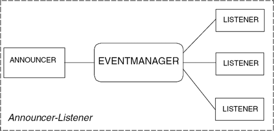
Listeners can choose to receive only a subset of the events announced by registering a "pattern" with the event manager. Only events that match the pattern are forwarded to the listener. The architecture can be applied recursively so that listeners also announce events to another set of listeners. In this way, an event dissemination "tree" can be constructed.
An important property of this architecture is that the announcer is insulated from knowledge of how many listeners there are and from which listeners are affected by a particular event. Listeners do not have to be processes; they may simply be objects in which a method is invoked as a result of an event. This mechanism is sometimes called implicit invocation since the announcer does not invoke listener methods explicitly. Listener methods are invoked implicitly as a result of an event announcement.
The Announcer–Listener architecture is widely used in user interface frameworks, and the Java Abstract Windowing Toolkit (AWT) is no exception. In section 11.3.2, we use the AWT event mechanism in an example program. In AWT, listeners are usually ordinary objects. Events, such as mouse clicks and button presses, cause methods to be invoked on objects. Our example uses events to control the execution of thread objects.
The model is defined for a fixed set of listeners and a fixed set of event patterns:
setListeners = {a,b,c,d}setPattern = {pat1,pat2}
The event manager is modeled by a set of REGISTER processes, each of which controls the registration and event propagation for a single, particular listener.
REGISTER = IDLE,
     IDLE = (register[p:Pattern] -> MATCH[p]
            |announce[Pattern]   -> IDLE
            ),

     MATCH[p:Pattern] =
            (announce[a:Pattern] ->
                if (a==p) then
                   (event[a] -> MATCH[p]
                   |deregister -> IDLE)
                else
                   MATCH[p]
            |deregister -> IDLE
            ).

     ||EVENTMANAGER = (Listeners:REGISTER)
                    /{announce/Listeners.announce}.
The REGISTER process ensures that the event action for a listener only occurs if the listener has previously registered, has not yet unregistered, and if the event pattern matches the pattern with which the listener registered. Figure 11.15 depicts the LTS for a:REGISTER for listener a.
The announcer is modeled as repeatedly announcing an event for one of the patterns defined by the Pattern set:
ANNOUNCER = (announce[Pattern] -> ANNOUNCER).
The listener initially registers for events of a particular pattern and then either performs local computation, modeled by the action compute, or receives an event. On receiving an event, the process either continues computing or deregisters and stops.
LISTENER(P='pattern) =
       (register[P] -> LISTENING),
     LISTENING =
       (compute  -> LISTENING
       |event[P] -> LISTENING
       |event[P] -> deregister -> STOP
       )+{register[Pattern]}.
ANNOUNCER_LISTENER describes a system with four listeners a, b, c, d, in which a and c register for events with pattern pat1 and b and d register for pat2.
||ANNOUNCER_LISTENER
                = ( a:LISTENER('pat1)
                  ||b:LISTENER('pat2)
                  ||c:LISTENER('pat1)
                  ||d:LISTENER('pat2)
                  ||EVENTMANAGER
                  ||ANNOUNCER
||Listeners:SAFE).The safety property, SAFE, included in the composite process ANNOUNCER_ LISTENER, asserts that each listener only receives events while it is registered and only those events with the pattern for which it registered. The property is defined below:
property
  SAFE = (register[p:Pattern]  -> SAFE[p]),
  SAFE[p:Pattern]= (event[p]   -> SAFE[p]
                   |deregister -> SAFE
                   ).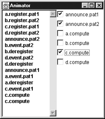
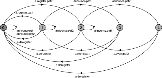
Safety analysis reveals that the system has no deadlocks or safety violations. A sample execution trace is shown in Figure 11.16.
The important progress property for this system is that the announcer should be able to announce events independently of the state of listeners, i.e. whether or not listeners are registered and whether or not listeners have stopped. We can assert this using the following set of progress properties:
progress ANNOUNCE[p:Pattern] = {announce[p]}Progress analysis using LTSA verifies that these properties hold for ANNOUNCER_ LISTENER.
To illustrate the use of the Announcer – Listener architecture, we implement the simple game depicted in Figure 11.17. The objective of the game is to hit all the moving colored blocks with the minimum number of mouse presses. A moving block is hit by pressing the mouse button when the mouse pointer is on top of the block. When a block is hit, it turns black and stops moving.
Each block is controlled by a separate thread that causes the block it controls to jump about the display at random. The threads also listen for mouse events that are announced by the display canvas in which the blocks move. These events are generated by the AWT and the program uses the AWT classes provided for event handling. The class diagram for the program is depicted in Figure 11.18.
Example 11.10. BoxCanvas class.
classBoxCanvasextendsCanvas {// clear all boxessynchronizedvoid reset(){...}// draw colored boxidat positionx,ysynchronizedvoid moveBox(int id, int x, int y){...}// draw black boxidat positionx,ysynchronizedvoid blackBox(int id, int x, int y){...} }
The display for the EventDemo applet is provided by the BoxCanvas class described in outline by Program 11.10.
The AWT interface MouseListener describes a set of methods that are invoked as a result of mouse actions. To avoid implementing all these methods, since we are only interested in the mouse-pressed event, we use the adapter class MouseAdapter which provides null implementations for all the methods in the MouseListener interface. MyClass extends MouseAdapter and provides an implementation for the mousePressed method. MyClass is an inner class of the BoxMover thread class; consequently, it can directly call private BoxMover methods. The code for BoxMover and MyListener is listed in Program 11.11.
The run() method of BoxMover repeatedly computes a random position and displays a box at that position. After displaying the box, waitHit() is called. This uses a timed wait() and returns for two reasons: either the wait delay expires and the value false is returned or isHit() computes that a hit has occurred and calls notify() in which case true is returned. Because MyListener is registered as a listener for events generated by the display, whenever the display announces a mouse-pressed event, MyListener.mousePressed() is invoked. This in turn calls isHit() with the mouse coordinates contained in the MouseEvent parameter.
If we compare the run() method with the LISTENER process from the model, the difference in behavior is the addition of a timeout action which ensures that after a delay, if no mouse event occurs, a new box position is computed and displayed. A model specific to the BoxMover thread is described by:
BOXMOVER(P='pattern) =
       (register[P] -> LISTENING),
     LISTENING =
       (compute->       // compute and display position
         (timeout -> LISTENING    // no mouse event
         |event[P] -> timeout -> LISTENING // miss
         |event[P] -> deregister -> STOP    // hit
         )
       )+{register[Pattern]}.
Example 11.11. BoxMover and MyListener classes.
importjava.awt.event.*;classBoxMoverextendsThread {privateBoxCanvas display;privateint id, delay, MaxX, MaxY, x, y;privateboolean hit=false;privateMyListener listener =newMyListener(); BoxMover(BoxCanvas d, int id, int delay) { display = d; this.id = id; this.delay=delay; display.addMouseListener(listener);// registerMaxX = d.getSize().width; MaxY = d.getSize().height; }private synchronizedvoid isHit(int mx, int my) { hit = (mx>x && mx<x+display.BOXSIZE && my>y && my<y+display.BOXSIZE);if(hit) notify(); }private synchronizedboolean waitHit()throwsInterruptedException { wait(delay);returnhit; }publicvoid run() {try{while(true) { x = (int)(MaxX*Math.random()); y = (int)(MaxY*Math.random()); display.moveBox(id,x,y);if(waitHit()) break; } }catch(InterruptedException e){} display.blackBox(id,x,y); display.removeMouseListener(listener);// deregister}classMyListenerextendsMouseAdapter {publicvoid mousePressed(MouseEvent e) { isHit(e.getX(),e.getY()); } } }
The reader should verify that the safety and progress properties for the ANNOUNCER_LISTENER still hold when BOXMOVER is substituted for LISTENER.
In this chapter, we have described three different concurrent architectures: Filter Pipeline, Supervisor – Worker and Announcer – Listener. A model was developed for each architecture and analyzed with respect to general properties such as absence of deadlock and correct termination. Guided by the models, we developed example programs to demonstrate how the components of each architecture interact during execution.
Each of the architectures uses a different type of connector to coordinate the communication between the components of the architecture. The Filter Pipeline uses pipes, which are essentially communication channels with zero or more buffers. We showed that the behavior of our primes sieve application, organized as a Filter Pipeline, was independent of the buffering provided in pipes. The components of the Supervisor – Worker architecture interact via a Linda tuple space, which is an unordered collection of data tuples. We provided a model of Linda tuple space and used it to investigate termination strategies for Supervisor – Worker systems. The Announcer – Listener components interact by event dissemination. We presented a general model of event dissemination and then used Java AWT events to implement the example program.
Pipes support one-to-one communication, tuple space supports any-to-any communication and event dissemination is one-to-many. These connectors were chosen as the most natural match with the topology of the architecture to which they were applied. However, it is possible, if not very natural, to use tuple space to implement a set of pipes and, more reasonably, to use rendezvous (section 10.3) instead of tuple space in the Supervisor – Worker architecture. In other words, for each architecture we have described one technique for organizing the communication between participating components. However, many variants of these architectures can be found in the literature, differing in the mechanisms used to support communication, how termination is managed and, of course, in the applications they support. A particular concurrent program may incorporate a combination of the basic architectures we have described here and in the rest of the book. For example, the filter processes in a pipeline may also be the clients of a server process.
As mentioned earlier, Filter Pipeline is the basic architecture used in the UNIX operating system to combine programs. The architecture is also used extensively in multimedia applications to process streams of video and audio information. An example of this sort of program can be found in Kleiman, Shah and Smaalders (1996). A discussion of the properties of more general pipe and filter networks may be found in Shaw and Garlan's book on Software Architecture (1996).
The Supervisor – Worker architecture appears in many guises in books and papers on concurrent programming. Andrews (1991) calls the architecture "replicated worker", Burns and Davies (1993) call it "process farm", while Carriero and Gelernter (1989b) characterize the form of parallelism supported by the architecture as "agenda parallelism". A paper by Cheung and Magee (1991) presents a simple way of assessing the likely performance of a sequential algorithm when parallelized using the Supervisor – Worker architecture. The paper also describes a technique for making the architecture fault-tolerant with respect to worker failure. The Supervisor – Worker architecture has been used extensively in exploiting the computational power of clusters of workstations.
A large literature exists on Linda (Gelernter, 1985; Carriero and Gelernter, 1989a, 1989b) and its derivatives. The proceedings of the "Coordination" series of conferences describe some of the current work on tuple-space-based models for concurrent programming, starting from the early conferences (Ciancarini and Hankin, 1996; Garlan and Le Metayer, 1997) and including more recent events (Nicola, Ferari and Meredith, 2004; Jacquet and Picco, 2005). The Linda tuple space paradigm clearly influenced the work on JavaSpacestrade (Freeman, Hupfer and Arnold, 1999).
Event-based architectures have been used to connect tools in software development environments (Reiss, 1990). As discussed in the chapter, windowing environments are usually event-based, as Smalltalk (Goldberg and Robson, 1983). In a distributed context, event processing forms an important part of network management systems (Sloman, 1994). Shaw and Garlan (1996) discuss some of the general properties of event-based systems.
11.1 N processes are required to synchronize their execution at some point before proceeding. Describe a scheme for implementing this barrier synchronization using Linda tuple space. Model the scheme using
TUPLESPACEand generate a trace to show the correct operation of your scheme.11.2 Describe a scheme for implementing the Supervisor – Worker architecture using rendezvous message-passing communication rather than tuple space.
(Hint: Make the Supervisor a server and the Workers clients.)
Model this scheme and show absence of deadlock and successful termination. Modify the Java example program to use
Entryrather thanTupleSpace.11.3 A process needs to wait for an event from either announcer A or announcer B, for example events indicating that button A or button B has been pressed, i.e.
(buttonA -> P[1] | buttonB -> P[2]).
Sketch the implementation of a Java thread that can block waiting for either of two events to occur. Assume initially that the Java events are handled by the same listener interface. Now extend the scheme such that events with different listener interfaces can be accommodated.
11.4 Provide a Java class which implements the following interface and has the behavior of
EVENTMANAGER:classListener {publicaction(int event); }interfaceEventManager { void announce(int event); void register(Listener x); void deregister(Listener x): }11.5 Each filter in a pipeline examines the stream of symbols it receives for a particular pattern. When one of the filters matches the pattern it is looking for the entire pipeline terminates. Develop a model for this system and show absence of deadlock and correct termination. Outline how your model might be implemented in Java, paying particular attention to termination.
11.6 A token ring is an architecture which is commonly used for allocating some privilege, such as access to a shared resource, to one of a set of processes at a time. The architecture works as follows:
A token is passed round the ring. Possession of the token indicates that that process has exclusive access to the resource. Each process holds on to the token while using the resource and then passes it on to its successor in the ring, or passes on the token directly if it does not require access.
Develop a model for this system and show absence of deadlock, exclusive access to the resource and access progress for every process. Is the system "buffer tolerant"? Outline how your model might be implemented in Java.
11.7 Consider a ring of nodes, each of which acts as a simplified replicated database (Roscoe, 1998). Each node can autonomously update its local copy. Updates are circulated round the ring to update other copies. It is possible that two nodes perform local updates at similar times and propagate their respective updates. This would lead to the situation where nodes receive updates in different orders, leading to inconsistent copies even after all the updates have propagated round the ring. Although we are prepared to tolerate copy inconsistency while updates are circulating, we cannot accept inconsistency that persists. To ensure consistent updates in the presence of node autonomy and concurrency, we require that, when quiescent (no updates are circulating and no node is updating its copy), all copies should have the same value.
In order to achieve this, we assign a priority to each update according to an (arbitrary) ordering of the originating node. Thus, in the case of clashes due to two simultaneous updates by different nodes, node i has priority over node j if i < j. Simultaneity is recognized by a node receiving an update while still having an outstanding update.
Develop a model for this system and show absence of deadlock and consistent values when quiescent.
(Hint: In order to keep the problem simple, let each node deal with only a single value. Updates are passed round the ring in the form: [j][x] where j=originator and x=update value. Nodes should be connected by channels which can be modeled as follows.)
constN = 3// number of nodesrangeNodes = 0..N-1constMax = 2// update valuesrangeValue = 0..Max-1 CHANNEL = (in[j:Nodes][x:Value]->out[j][x]->CHANNEL).