
In Chapter 1, we noted that in concurrent programs, computational activities are permitted to overlap in time and that the subprogram executions describing these activities proceed concurrently. The execution of a program (or subprogram) is termed a process and the execution of a concurrent program thus consists of multiple processes. In this chapter, we define how processes can be modeled as finite state machines. We then describe how processes can be programmed as threads, the form of process supported by Java.
A process is the execution of a sequential program. The state of a process at any point in time consists of the values of explicit variables, declared by the programmer, and implicit variables such as the program counter and contents of data/address registers. As a process executes, it transforms its state by executing statements. Each statement consists of a sequence of one or more atomic actions that make indivisible state changes. Examples of atomic actions are uninterruptible machine instructions that load and store registers. A more abstract model of a process, which ignores the details of state representation and machine instructions, is simply to consider a process as having a state modified by indivisible or atomic actions. Each action causes a transition from the current state to the next state. The order in which actions are allowed to occur is determined by a transition graph that is an abstract representation of the program. In other words, we can model processes as finite state machines.
Figure 2.1 depicts the state machine for a light switch that has the actions on and off. We use the following diagrammatic conventions. The initial state is always numbered 0 and transitions are always drawn in a clockwise direction. Thus in Figure 2.1, on causes a transition from state (0) to state (1) and off causes a transition from state (1) to state (0). This form of state machine description is known as a Labeled Transition System (LTS), since transitions are labeled with action names. Diagrams of this form can be displayed in the LTS analysis tool, LTSA. Although this representation of a process is finite, the behavior described need not be finite. For example, the state machine of Figure 2.1 allows the following sequence of actions:
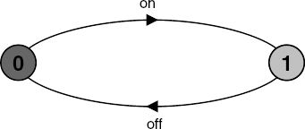
on→off→on→off→on→off→ ...
The graphical form of state machine description is excellent for simple processes; however, it becomes unmanageable (and unreadable) for large numbers of states and transitions. Consequently, we introduce a simple algebraic notation called FSP (Finite State Processes) to describe process models. Every FSP description has a corresponding state machine (LTS) description. In this chapter, we will introduce the action prefix and choice operators provided by FSP. The full language definition of FSP may be found in Appendix B.
Note
If x is an action and P a process then the action prefix (x->P) describes a process that initially engages in the action x and then behaves exactly as described by P.
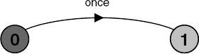
The action prefix operator "->" always has an action on its left and a process on its right. In FSP, identifiers beginning with a lowercase letter denote actions and identifiers beginning with an uppercase letter denote processes. The following example illustrates a process that engages in the action once and then stops:
ONESHOT = (once->STOP).
Figure 2.2 illustrates the equivalent LTS state machine description for ONESHOT. It shows that the action prefix in FSP describes a transition in the corresponding state machine description. STOP is a special predefined process that engages in no further actions, as is clear in Figure 2.2. Process definitions are terminated by ".".
Repetitive behavior is described in FSP using recursion. The following FSP process describes the light switch of Figure 2.1:
SWITCH = OFF,
OFF    = (on  ->ON),
ON     = (off->OFF).
As indicated by the "," separators, the process definitions for ON and OFF are part of and local to the definition for SWITCH. It should be noted that these local process definitions correspond to states in Figure 2.1. OFF defines state (0) and ON defines state(1). A more succinct definition of SWITCH can be achieved by substituting the definition of ON in the definition of OFF:
SWITCH = OFF,
OFF    = (on ->(off->OFF)).
Finally, by substituting SWITCH for OFF, since they are defined to be equivalent, and dropping the internal parentheses we get:
SWITCH = (on->off->SWITCH).
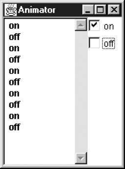
These three definitions for SWITCH generate identical state machines (Figure 2.1). The reader can verify this using the LTS analysis tool, LTSA, to draw the state machine that corresponds to each FSP definition. The definitions may also be animated using the LTSA Animator to produce a sequence of actions. Figure 2.3 shows a screen shot of the LTSA Animator window. The animator lets the user control the actions offered by a model to its environment. Those actions that can be chosen for execution are ticked. In Figure 2.3, the previous sequence of actions, shown on the left, has put the SWITCH in a state where only the on action can occur next. We refer to the sequence of actions produced by the execution of a process (or set of processes) as a trace.
The process TRAFFICLIGHT is defined below with its equivalent state machine representation depicted in Figure 2.4.
TRAFFICLIGHT =
    (red->orange->green->orange->TRAFFICLIGHT).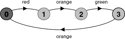
In general, processes have many possible execution traces. However, the only possible trace of the execution of TRAFFICLIGHT is:
red→orange→green→orange→red→orange→green ...
To allow a process to describe more than a single execution trace, we introduce the choice operator.
Note
If x and y are actions then (x->P|y->Q) describes a process which initially engages in either of the actions x or y. After the first action has occurred, the subsequent behavior is described by P if the first action was x and Q if the first action was y.
The following example describes a drinks dispensing machine which dispenses hot coffee if the red button is pressed and iced tea if the blue button is pressed.
DRINKS = (red->coffee->DRINKS
         |blue->tea->DRINKS
         ).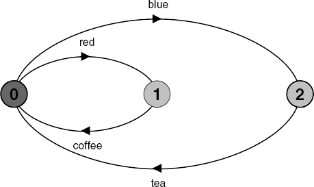
Figure 2.5 depicts the graphical state machine description of the drinks dispenser. Choice is represented as a state with more than one outgoing transition. The initial state has two possible outgoing transitions labeled red and blue. Who or what makes the choice as to which action is executed? In this example, the environment makes the choice – someone presses a button. We will see later that a choice may also be made internally within a process. The reader may also question at this point if there is a distinction between input and output actions. In fact, there is no semantic difference between an input action and an output action in the models we use. However, input actions are usually distinguished by forming part of a choice offered to the environment while outputs offer no choice. In the example, red and blue model input actions and coffee and tea model output actions. Possible traces of DRINKS include:
red→coffee→red→coffee→red→coffee......
blue→tea→blue→tea→blue→tea......
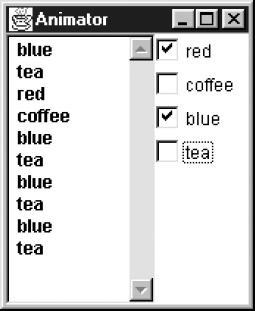
blue→tea→red→coffee→blue→tea→blue→tea......As before, the LTSA Animator can be used to animate the model and produce a trace, as indicated in Figure 2.6. In this case, both red and blue actions are ticked as both are offered for selection.
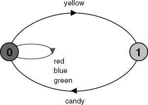
A state may have more than two outgoing transitions; hence the choice operator "|" can express a choice of more than two actions. For example, the following process describes a machine that has four colored buttons only one of which produces an output.
FAULTY = (red ->FAULTY
              |blue ->FAULTY
              |green->FAULTY
              |yellow->candy->FAULTY
              ).
The order of elements in the choice has no significance. The FAULTY process may be expressed more succinctly using a set of action labels. The set is interpreted as being a choice of one of its members. Both definitions of FAULTY generate exactly the same state machine graph as depicted in Figure 2.7. Note that red, blue and green label the same transition back to state (0).
FAULTY = ({red,blue,green}-> FAULTY
              |yellow -> candy -> FAULTY
              ).
The process (x->P|x->Q) is said to be non-deterministic since after the action x, it may behave as either P or Q. The COIN process defined below and drawn as a state machine in Figure 2.8 is an example of a non-deterministic process.
COIN = (toss -> heads -> COIN
            |toss -> tails -> COIN
            ).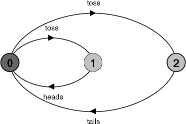
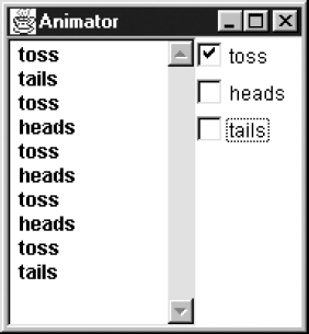
After a toss action, the next action may be either heads or tails. Figure 2.9 gives a sample trace for the COIN process.
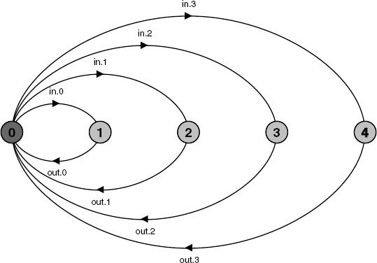
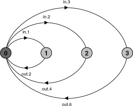
In order to model processes and actions that can take multiple values, both local processes and action labels may be indexed in FSP. This greatly increases the expressive power of the notation. Indices always have a finite range of values that they can take. This ensures that the models we describe in FSP are finite and thus potentially mechanically analyzable. The process below is a buffer that can contain a single value – a single-slot buffer. It inputs a value in the range 0 to 3 and then outputs that value.
BUFF = (in[i:0..3]->out[i]-> BUFF).
The above process has an exactly equivalent definition in which the choice between input values is stated explicitly. The state machine for both of these definitions is depicted in Figure 2.10. Note that each index is translated into a dot notation "." for the transition label, so that in[0] becomes in.0, and soon.
BUFF = (in[0]->out[0]->BUFF
        |in[1]->out[1]->BUFF
        |in[2]->out[2]->BUFF
        |in[3]->out[3]->BUFF
        ).
Another equivalent definition, which uses an indexed local process, is shown below. Since this uses two index variables with the same range, we declare a range type.
range T = 0..3

BUFF       = (in[i:T]->STORE[i]),
STORE[i:T] = (out[i] ->BUFF).
The scope of a process index variable is the process definition. The scope of an action label index is the choice element in which it occurs. Consequently, the two definitions of the index variable i in BUFF above do not conflict. Both processes and action labels may have more than one index. The next example illustrates this for a process which inputs two values, a and b, and outputs their sum. Note that the usual arithmetic operations are supported on index variables.
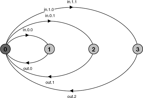
constN = 1rangeT = 0..NrangeR = 0..2*N SUM = (in[a:T][b:T]->TOTAL[a+b]), TOTAL[s:R] = (out[s]->SUM).
We have chosen a small value for the constant N in the definition of SUM to ensure that the graphic representation of Figure 2.11 remains readable. The reader should generate the SUM state machine for larger values of N to see the limitation of graphic representation.
Processes may be parameterized so that they may be described in a general form and modeled for a particular parameter value. For instance, the single-slot buffer described in section 2.1.3 and illustrated in Figure 2.10 can be described as a parameterized process for values in the range 0 to N as follows:
BUFF(N=3) = (in[i:0..N]->out[i]-> BUFF).
Parameters must be given a default value and must start with an uppercase letter. The scope of the parameter is the process definition. Alternatively, N may be given a fixed, constant value. This may be more appropriate if N is to be used in more than one process description.
const N = 3
BUFF = (in[i:0..N]->out[i]-> BUFF).It is often useful to define particular actions as conditional, depending on the current state of the machine. We use Boolean guards to indicate that a particular action can only be selected if its guard is satisfied.
Note
The choice (when Bx ->P | y ->Q) means that when the guard B is true then the actions x and y are both eligible to be chosen, otherwise if B is false then the action x cannot be chosen.
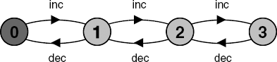
The example below (with its state machine depicted in Figure 2.12) is a process that encapsulates a count variable. The count can be increased by inc operations and decreased by dec operations. The count is not allowed to exceed N or be less than zero.
COUNT (N=3)   = COUNT[0],
     COUNT[i:0..N] = (when(i<N)  inc->COUNT[i+1]
                     |when(i>0)  dec->COUNT[i-1]
                     ).
FSP supports only integer expressions; consequently, the value zero is used to represent false and any non-zero value represents true. Expression syntax is the same as C, C++ and Java.
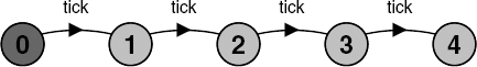
In section 2.2, which describes how processes can be implemented in Java, we outline the implementation of a countdown timer. The timer, once started, outputs a tick sound each time it decrements the count and a beep when it reaches zero. At any point, the countdown may be aborted by a stop action. The model for the countdown timer is depicted below; the state machine is in Figure 2.13.
COUNTDOWN (N=3)   = (start-> COUNTDOWN[N]),
    COUNTDOWN[i:0..N] = (when(i>0) tick-> COUNTDOWN[i-1]
                        |when(i==0) beep-> STOP
                        |stop-> STOP
                        ).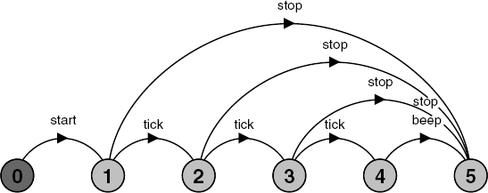
The set of possible traces of COUNTDOWN are as given below.
start→stop
     start→tick→stop
     start→tick→tick→stop
     start→tick→tick→tick→stop
     start→tick→tick→tick→beep
(Note that the LTSA Animator reports the STOP state as DEADLOCK. Deadlock is a more general situation where a system of processes can engage in no further actions. It is discussed later, in Chapter 6.)
For example, the alphabet of the COUNTDOWN process of the previous section is {start, stop, tick, beep}. A process may only engage in the actions in its alphabet; however, it may have actions in its alphabet in which it never engages. For example, a process that writes to a store location may potentially write any 32-bit value to that location; however, it will usually write a more restricted set of values. In FSP, the alphabet of a process is determined implicitly by the set of actions referenced in its definition. We will see later in the book that it is important to be precise about the alphabet of a process.
How do we deal with the situation described above in which the set of actions in the alphabet is larger than the set of actions referenced in its definition? The answer is to use the alphabet extension construct provided by FSP. The process WRITER defined below uses the actions write[1] and write[3] in its definition but defines an alphabet extension "+{...}" of the actions write[0..3]. The alphabet of a process is the union of its implicit alphabet and any extension specified. Consequently, the alphabet of WRITER is write[0..3].
WRITER = (write[1]->write[3]->WRITER)
              +{write[0..3]}.
It should be noted that where a process is defined using one or more local process definitions, the alphabet of each local process is exactly the same as that of the enclosing process. The alphabet of the enclosing process is simply the union of the set of actions referenced in all local definitions together with any explicitly specified alphabet extension.
At the beginning of this chapter, we introduced a process as being the execution of a program or subprogram. In the previous section, we described how a process could be modeled as a finite state machine. In this section, we will see how processes are represented in computing systems. In particular, we describe how processes are programmed in Java.
The term process, meaning the execution of a program, originates in the literature on the design of operating systems. A process in an operating system is a unit of resource allocation both for CPU time and for memory. A process is represented by its code, data and the state of the machine registers. The data of the process is divided into global variables and local variables organized as a stack. Generally, each process in an operating system has its own address space and some special action must be taken to allow different processes to access shared data. The execution of an application program in an operating system like Unix involves the following activities: allocating memory (global data and stack) for the process, loading some or all of its code into memory and running the code by loading the address of the initial instruction into the program counter register, the address of its stack into the stack pointer register and so on. The operating system maintains an internal data structure called a process descriptor which records details such as scheduling priority, allocated memory and the values of machine registers when the process is not running.
The above description does not conflict with our previous conception of a process, it is simply more concrete. This traditional operating system process has a single thread of control – it has no internal concurrency. With the advent of shared memory multiprocessors, operating system designers have catered for the requirement that a process might require internal concurrency by providing lightweight processes or threads. The name thread comes from the expression "thread of control". Modern operating systems like Windows NT permit an operating system process to have multiple threads of control.
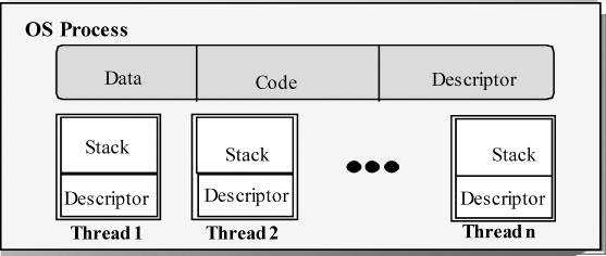
The relationship between heavyweight operating system (OS) processes and lightweight processes or threads is depicted in Figure 2.14. The OS process has a data segment and a code segment; however, it has multiple stacks, one for each thread. The code for a thread is included in the OS process code segment and all the threads in a process can access the data segment. The Java Virtual Machine, which of course usually executes as a process under some operating system, supports multiple threads as depicted in Figure 2.14. Each Java thread has its own local variables organized as a stack and threads can access shared variables.
In the previous section, we modeled processes as state machines. Since threads are simply a particular implementation of the general idea of a process as an executing program, they too can be modeled as state machines. They have a state, which they transform by performing actions (executing instructions). To avoid confusion in the rest of the book, we will use the term process when referring to models of concurrent programs and the term thread when referring to implementations of processes in Java.
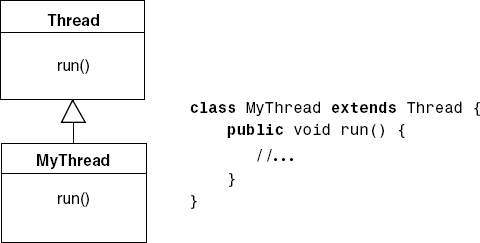
The operations to create and initialize threads and to subsequently control their execution are provided by the Java class Thread in the package java.lang. The program code executed by a thread is provided by the method run(). The actual code executed depends on the implementation provided for run() in a derived class, as depicted in the class diagram of Figure 2.15.
The class diagrams we use in this book are a subset of the Unified Modeling Language, UML (Fowler and Scott, 1997; Booch, Rumbaugh and Jacobson, 1998). For those unfamiliar with this notation, a key may be found in Appendix D.
Since Java does not permit multiple inheritance, it is sometimes more convenient to implement the run() method in a class not derived from Thread but from the interface Runnable as depicted in Figure 2.16.
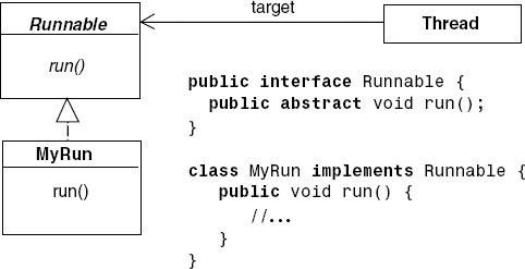
A Java Thread object is created by a call to new in the same way that any other Java object is constructed. The two ways of creating a thread corresponding to Figures 2.15 and 2.16 respectively are:
Thread a =newMyThread(); Thread b =newThread(newMyRun());
The thread constructor may optionally take a string argument to name the thread. This can be useful for debugging but has no other role. The following outlines the states (in italics) in which a thread may exist and the operations provided by the Thread class to control a thread.
Once created,
start()causes a thread to call itsrun()method and execute it as an independent activity, concurrent with the thread which calledstart().A thread terminates when the
run()method returns or when it is stopped bystop(). A terminated thread may not be restarted. A thread object is only garbage collected when there are no references to it and it has terminated.The predicate
isAlive()returns true if a thread has been started but has not yet terminated.When started, a thread may be currently running on the processor, or it may be runnable but waiting to be scheduled. A running process may explicitly give up the processor using
yield().Athreadmaybe non-runnable as a result of being suspended using
suspend(). It can be made runnable again usingresume().sleep()causes a thread to be suspended (made non-runnable) for a given time (specified in milliseconds) and then automatically resume (be made runnable).
This is not a complete list of operations provided by the Thread class. For example, threads may be given a scheduling priority. We will introduce these extra operations later in the book, as they are required.
We can use FSP to give a concise description of the thread life cycle as shown below. The actions shown in italics are not methods from class Thread. Taking them in order of appearance: end represents the action of the run() method returning or exiting, run represents a set of application actions from the run() method and dispatch represents an action by the Java Virtual Machine to run a thread on the processor.
THREAD       = CREATED,
   CREATED      = (start          ->RUNNABLE
                  |stop           ->TERMINATED),
   RUNNING      = ({suspend,sleep}->NON_RUNNABLE
                  |yield          ->RUNNABLE
                  |{stop, end}     ->TERMINATED
                  |run            ->RUNNING),
RUNNABLE = (suspend ->NON_RUNNABLE|dispatch ->RUNNING
|stop ->TERMINATED),
NON_RUNNABLE = (resume ->RUNNABLE
|stop ->TERMINATED),
TERMINATED = STOP.The corresponding state machine is depicted in Figure 2.17. States 0 to 4 correspond to CREATED, TERMINATED, RUNNABLE, RUNNING and NON_RUNNABLE respectively.

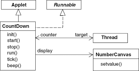
The model for a timer which counts down to zero and then beeps was described in section 2.1.5 (Figure 2.13). In this section, we describe the implementation of the countdown timer as a thread that is created by a Java applet. The class diagram for the timer is depicted in Figure 2.18.
NumberCanvas is a display canvas that paints an integer value on the screen. An outline of the class, describing the methods available to users, is presented in Program 2.1. It is the first of a set of display classes that will be used throughout the book. The full code for these classes can be found on the website that accompanies this book (http://www.wileyeurope.com/college/magee).
Example 2.1. NumberCanvas class.
public classNumberCanvasextendsCanvas {// create canvas with title and optionally set background colorpublicNumberCanvas(String title) {...}publicNumberCanvas(String title, Color c) {...}//set background colorpublicvoid setcolor(Color c){...}//displaynewvalon screenpublicvoid setvalue(int newval){...} }
The code for the CountDown applet is listed in Program 2.2.
Example 2.2. CountDown applet class.
public classCountDownextendsAppletimplementsRunnable { Thread counter; int i;final staticint N = 10; AudioClip beepSound, tickSound; NumberCanvas display;publicvoid init() { add(display=newNumberCanvas("CountDown"));
display.resize(150,100);
      tickSound =
        getAudioClip(getDocumentBase(),"sound/tick.au");
      beepSound =
        getAudioClip(getDocumentBase(),"sound/beep.au");
    }

    public void start() {
      counter = new Thread(this);
      i = N; counter.start();
    }

    public void stop() {
      counter = null;
    }

    public void run() {
      while(true) {
        if (counter == null) return;
        if (i>0)  { tick(); --i; }
        if (i==0) { beep(); return;}
      }
    }

    private void tick(){
      display.setvalue(i); tickSound.play();
      try{ Thread.sleep(1000);}
      catch (InterruptedException e){}
    }

    private void beep(){
      display.setvalue(i); beepSound.play();
    }
  }
The counter thread is created and started running by the start() method when the CountDown applet is started by the Web browser in which it executes. CountDown implements the Runnable interface by providing the method run() which defines the behavior of the thread. To permit easy comparison between the COUNTDOWN model and the behavior implemented by the run() method, the model is repeated below:
COUNTDOWN (N=3)   = (start-> COUNTDOWN[N]),
     COUNTDOWN[i:0..N] = (when(i>0) tick-> COUNTDOWN[i-1]
                         |when(i==0) beep-> STOP
                         |stop-> STOP
                         ).
The thread counter.start() method causes the run() method to be invoked. Hence, just as the start action in the model is followed by COUNTDOWN[i], sothe run() method is an implementation of the COUNTDOWN[i] process. The index of the process COUNTDOWN[i] is represented by the integer field i. The recursion in the model is implemented as a Java while loop. Guarded choice in COUNTDOWN[i] is implemented by Java if statements. Note that we have reordered the conditions from the model, since in the implementation, they are evaluated sequentially. If the thread is stopped, it must not perform any further actions. In Chapters 4 and 5, we will see a different way of implementing choice when a model process is not implemented as a thread.
When run() returns the thread terminates – this corresponds to the model process STOP. This can happen for two reasons: either i==0 or the thread reference counter becomes null. It can become null if the browser invokes the stop() method – usually as a result of a user requesting a change from the Web page in which the applet is active. The stop() method sets counter to null. This method of stopping a thread is preferable to using the Thread.stop() method since it allows a thread to terminate gracefully, performing cleanup actions if necessary. Thread.stop() terminates a thread whatever state it is in, giving it no opportunity to release resources. Melodramatically, we may think of Thread.stop() as killing the thread and the technique we have used as equivalent to requesting the thread to commit suicide! For these reasons, Sun have suggested that Thread.stop() be "deprecated". This means that it may not be supported by future Java releases.
The implementation of tick() displays the value of i, plays the tick sound and then delays the calling thread for 1000 milliseconds (one second) using Thread.sleep(). This is a class method since it always operates on the currently running thread. The method sleep() can terminate abnormally with an InterruptedException. The code of Program 2.2 simply provides an exception handler that does nothing.
The implementation of beep() displays i and plays the beep sound. The tick() and beep() methods correspond to the tick and beep actions of the model. An implementation must fill in the details that are abstracted in a model.
This chapter has introduced the concept of a process, explained how we model processes and described Java threads as implementations of processes. In particular:
The execution of a program (or subprogram) is termed a process. Processes are the units of concurrent activity used in concurrent programming.
A process can be modeled as a state machine in which the transitions are atomic or indivisible actions executed by the process. We use LTS, Labeled Transition Systems, to represent state machines.
State machines are described concisely using FSP, a simple process algebra. The chapter introduced the action prefix, "
->", and choice, "|", operators in addition to the use of recursion, index sets and guards.Our notations do not distinguish input actions from outputs. However, inputs usually form part of a choice offered to the environment of a process while outputs do not.
We have used Java threads to show how processes are implemented and how they are used in programs. Java threads are an example of lightweight processes, in the terminology of operating systems.
The use of state machines as an abstract model for processes is widely used in the study of concurrent and distributed algorithms. For example, in her book Distributed Algorithms, Nancy Lynch (1996) uses I/O automata to describe and reason about concurrent and distributed programs. I/O automata are state machines in which input, output and internal actions are distinguished and in which input actions are always enabled (i.e., they are offered as a choice to the environment in all states). The interested reader will find an alternative approach to modeling concurrent systems in that book.
State machines are used as a diagrammatic aid (usually as State Transition Diagrams, STD) in most design methods to describe dynamic activity. They can be extended to cater for concurrency. An interesting and widely used form is statecharts (Harel, 1987), designed by David Harel and incorporated in the STATEMATE software tool (Harel, Lachover, Naamad, et al., 1990) for the design of reactive systems. A form of this notation has been adopted in the Unified Modeling Language, UML, of Booch, Rumbaugh and Jacobson (1998). See http://www.uml.org/.
The association of state machines with process algebra is due to Robin Milner (1989) who gives an operational semantics for a Calculus of Communicating Systems (CCS) using Labeled Transition Systems in his inspirational book Communication and Concurrency. While we have adopted the CCS approach to semantics, the syntax of FSP owes more to C.A.R. Hoare's CSP presented in Communicating Sequential Processes (1985). The semantic differences between FSP and its antecedents, CCS and CSP, are documented and explained in succeeding chapters. The syntactic differences are largely due to the requirement that FSP be easily parsed by its support tool LTSA.
Process algebra has also been used in formal description languages such as LOTOS (ISO/IEC, 1988). LOTOS is an ISO standard language for the spec-ification of distributed systems as interacting processes. As in FSP, process behavior is described using action prefix and choice operators, guards and recursion. However, unlike FSP, LOTOS includes facilities for defining abstract data types. Naive use of the data type part of LOTOS quickly leads to intractable models.
FSP was specifically designed to facilitate modeling of finite state processes as Labeled Transition Systems. LTS provides the well-defined mathematical properties that facilitate formal analysis. LTSA provides automated support for displaying and animating the examples in this chapter. Later in the book we will see how LTSA can be used for verifying properties using model checking.
The reader interested in more details on Java should consult the information on-line from JavaSoft. For more on the pragmatics of concurrent programming in Java, see Doug Lea's book Concurrent Programming in Java ™: Design Principles and Patterns (1999).
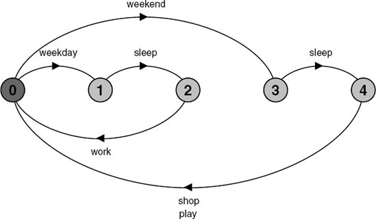
2.1 For each of the following processes, give the Finite State Process (FSP) description of the Labeled Transition System (LTS) graph. The FSP process descriptions may be checked by generating the corresponding state machines using the analysis tool, LTSA.
MEETING
JOB
GAME
MOVE
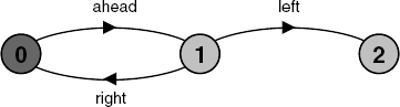
DOUBLE
FOURTICK
PERSON
2.2 A variable stores values in the range 0..N and supports the actions read and write. Model the variable as a process,
VARIABLE, using FSP.For N=2, check that it can perform the actions given by the trace:
write.2→read.2→read.2→write.1→write.0→read.0
2.3 A bistable digital circuit receives a sequence of trigger inputs and alternately outputs 0 and 1. Model the process
BISTABLEusing FSP, and check that it produces the required output; i.e., it should perform the actions given by the trace:trigger→1→trigger→0→trigger→1→trigger→0 ...
(Hint: The alphabet of
BISTABLEis{[0],[1],trigger}.)2.4 A sensor measures the water level of a tank. The level (initially 5) is measured in units 0..9. The sensor outputs a low signal if the level is less than 2 and a high signal if the level is greater than 8 otherwise it outputs normal. Model the sensor as an FSP process,
SENSOR.(Hint: The alphabet of
SENSORis{level[0..9], high, low, normal}.)2.5 A drinks dispensing machine charges 15p for a can of Sugarola. The machine accepts coins with denominations 5p, 10p and 20p and gives change. Model the machine as an FSP process,
DRINKS.2.6 A miniature portable FM radio has three controls. An on/off switch turns the device on and off. Tuning is controlled by two buttons
scanandresetwhich operate as follows. When the radio is turned on orresetis pressed, the radio is tuned to the top frequency of the FM band (108 MHz). Whenscanis pressed, the radio scans towards the bottom of the band (88 MHz). It stops scanning when itlockson to a station or it reaches the bottom (end). If the radio is currently tuned to a station andscanis pressed then it starts to scan from the frequency of that station towards the bottom. Similarly, whenresetis pressed the receiver tunes to the top. Using the alphabet{on, off, scan, reset, lock, end}, model the FM radio as an FSP process,RADIO.For each of the exercises 2.2 to 2.6, draw the state machine diagram that corresponds to your FSP specification and check that it can perform the required actions. The state machines may be drawn manually or generated using the analysis tool, LTSA. LTSA may also be used to animate (run) the specification to produce a trace.
2.7 Program the radio of exercise 2.6 in Java, complete with graphic display.