
The Visual Simulation Environment, a key part of Microsoft Robotics Developer Studio, uses 3D graphics to render a virtual world and a physics engine to approximate interactions between objects within that world. At first glance, it looks something like a game engine. However, after a little bit of use, it quickly becomes apparent that it is much different; whereas many actions and events are scripted in a game environment, the things that happen in the simulator rely completely on the interactions and motions of objects in the environment.
This chapter explains how to use the Visual Simulation Environment along with all of the simulation objects and services provided in the SDK. Subsequent chapters explain in detail how you can add your own objects and environments to the simulator to explore your own robotic designs.
In this chapter, you'll learn the following:
How the simulator can help you prototype new algorithms and robots
What hardware and software are required to run the simulator
How to use the basic simulator functions
How to use the Simulation Editor to place robots and other entities in a new environment
What built-in entities are provided with the SDK and how to use them
This chapter focuses on using the simulator functionality with the environments and entities provided as part of the SDK. The next chapters go into more detail about how you define your own environment and entities.
The simulator is a great place to prototype new robot designs, offering many advantages:
Prototyping new robots in the real world is a task full of soldering irons and nuts and bolts. Moving from one iteration of a design to the next can take weeks or months. In the simulator, you can easily make several changes and refinements to a design in just a day or two.
The simulator enables you to easily design and debug software. It is often difficult to have a debugger connected to a robot under motion, making it difficult to determine just what went wrong when the robot suddenly decides to ram the nearest wall. When your robot is running in the simulation environment, it is easy to set breakpoints on the services that control it and to find the bugs in your code. Once you have your algorithms debugged and tuned in the simulator, it is often possible to run the exact same code on your actual robot.
The simulator can be particularly useful in a classroom scenario in which you have several students who need to use a robot and only limited hardware available. Students can spend most of their time writing software and debugging the behavior of a simulated robot before testing the final version on the actual hardware. This is also a very useful feature when a new robot is being developed for which only one or two prototypes are available but several people need to write software for the new robot.
Another advantage to simulation is personal safety. An intern once demonstrated how he had programmed a real-world Pioneer 3DX robot to determine the direction of his voice using a microphone array. The robot would respond to spoken commands such as "Come here!" or "Stop!" Unfortunately, the robot was a little slow to respond to the stop command and it nearly pinned the intern against the wall before he could hit the reset switch. The simulator provides a way to debug your robot without risking bodily injury. Moreover, if your robot suddenly achieves self-awareness and starts running amok while yelling "Destroy all humans!" you won't need to call out the National Guard to subdue him if he is confined to the simulator.
It would be nice to able to tell you that the simulation environment will bring world peace and solve embarrassing hygiene problems, but you should be aware that it does have some limitations:
The physics engine is remarkably good at solving complicated object dynamics and collisions. The real world, however, is a very complicated place, and it is certainly possible to define a simulation scene that is difficult for the physics engine to process in its allotted time. The physics model for a scene is, by necessity, much more simplified than its real-world counterpart. A complicated object composed of many pieces may be modeled as a simple cube or sphere in the simulation world. You need to make careful decisions about where to add detail to your simulated world to increase the fidelity of the simulation while still allowing it to run at a reasonable rate.
The real world is a very noisy place. Real sensors often return noisy data. Real gears and wheels sometimes slip, and real video cameras often return images with bad pixels. Good robotics algorithms need to account for these issues, but they are often not present in the simulator. A simulated IR sensor is only as noisy as you have programmed it to be. A simulated camera will return more consistent and noise-free images than a real camera. In addition, the simulated world is often more visually simple than the real world, so image-processing algorithms have an easier time interpreting images from the simulated world.
You should consider the difference in computing power between the simulation environment and the actual robot. The simulator may run on a powerful desktop computer with a very fast CPU, while the actual robot might have a much slower CPU with slower data busses. A simulated camera may deliver 60 frames per second of video while a real camera might be limited to 1–2 frames per second. When designing algorithms, it is important to consider the performance and limitations of the final hardware.
Your experience with the simulator will be much better if you have the proper software and hardware to run it well. If the simulator cannot run, it displays a red window with some text indicating what problem it encountered. The problem may be due to insufficient hardware capability or a software configuration problem. This section details the hardware and software requirements you'll need to run the simulator.
When the simulator displays the red screen, it will be unable to draw the graphical environment on the screen but will continue to run the physics part of the simulation. As you will see, it is quite easy to query the state of the simulation to find out what is happening. In other words, the simulator may still be useful even if it is unable to display the graphics.
At a minimum, you must have a graphics card that is capable of running pixel and vertex shader programs of version 2.0 or higher. Video cards are often rated according to the version of DirectX that they support. If your card supports only DirectX 8, then it will not run the simulator. If your card supports DirectX 9, then you need to check which versions of pixel and vertex shaders are supported. Some older cards only support version 1.0 or 1.1 and will not run the simulator. If your card supports version 2.0 or 3.0 shaders or it supports DirectX 10, it should run the simulator well. Most mid- or upper-range graphics cards sold within the past couple of years have sufficient power.
One caveat here is that some newer laptops and even desktop machines have mobile or other specialized chipsets that may not run the simulator even though they are fairly new. This is because these machines are primarily intended for word processing or web browsing and they don't have high-performance 3D graphics capabilities.
The best way to determine the capabilities of your graphics card is to do the following:
Right-click the Windows desktop to bring up the Display Properties.
Click the Settings tab to see the name of your video card. Alternatively, you can bring up the Hardware Device Manager from the Windows Control Panel.
Expand the Display Adapters item to see the name of your video card.
Go to the website of the card manufacturer and search on the video card name. The manufacturer often provides detailed specifications for fairly recent cards.
If you are unable to find more information directly from the manufacturer, several websites list the capabilities of various video cards. You can go to the following website to find information on nVidia, ATI, and Matrox video cards: www.techpowerup.com/gpudb.
If your video card appears to meet the requirements just described and the simulator still fails to run, you may have a software configuration problem.
All of the software required to run the simulator is installed as part of the Microsoft Robotics Developer Studio SDK. Figure 5-1 shows the final screen of the installer. When you install the SDK, be sure to check the box to install the AGEIA PhysX engine, as well as Microsoft XNA and Microsoft DirectX. It is recommended that you also check the boxes to install the other components.
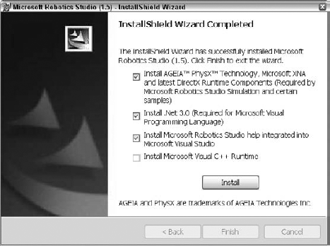
The XNA and DirectX installers require an active Internet connection. If your machine did not have an Internet connection during installation, it may be necessary to go back and manually install these components. Alternatively, you can uninstall and reinstall the SDK when you do have an Internet connection.
Version 1.5 of the MRDS Visual Simulation Environment requires the following additional software:
The following sections discuss this additional software.
The simulator uses the AGEIA PhysX engine to simulate physical interactions within the virtual environment. It requires version 2.7.0 of the PhysX engine. You can see which version you have installed by selecting the AGEIA item from the Start menu and then selecting ageia PhysX Properties. Make sure that V2.7.0 is displayed as one of the installed versions on the Info tab. You can also run the simple demo on the Demo tab to verify that the engine is working properly.
One of the great features of the AGEIA PhysX engine is that it can be accelerated with specialized hardware. You can find out more about this option on the AGEIA website at www.ageia.com. You can also download the latest AGEIA run-time drivers from www.ageia.com/drivers/drivers.html.
You may find it useful to download the entire AGEIA development SDK to learn more about how the physics engine works. While the PhysX APIs are not directly exposed by the simulator, an understanding of the engine and the objects it supports is very helpful. It is necessary to register before downloading the PhysX SDK from the following website: www.ageia.com/developers/downloads.html.
The Microsoft XNA library is a managed code implementation of the DirectX APIs. The simulator uses the Microsoft XNA Framework, which is a set of APIs that provide access to the underlying DirectX subsystem from managed code.
MRDS version 1.5 requires version 1.0 of the XNA Framework or the version 1.0 refresh, which was made available on April 24, 2007. You can find a link to the download page for the XNA Framework on the XNA Game Studio Express page at http://msdn2.microsoft.com/en-us/xna/aa937795.aspx. Alternatively, you can go to the XNA home page (www.microsoft.com/xna) and search for the framework download.
You may also find it helpful to download the XNA Game Studio Express SDK, which provides documentation on XNA classes and APIs. Some of these are used in the simulation entity sample code provided in the MRDS SDK. A link to the download page for XNA Game Studio Express can be found on the web page referenced above.
DirectX is a set of system APIs that provide access to graphics, sound, and input devices. The simulator in MRDS version 1.5 requires a DirectX runtime at least as recent as April, 2007. You can find the download link for this by loading the following page and searching for "DirectX Redist (April 2007)" on www.microsoft.com/downloads.
You may also find it helpful to download the entire DirectX SDK. This SDK includes a variety of tools that aid in making texture maps and other content for simulator scenes. You can find a download link for this by loading the aforementioned page and searching for "DirectX SDK – (April 2007)."
The easiest way to get the simulator up and running is to run it from the Start menu. Select the Visual Simulation Environment item from the Microsoft Robotics Developer Studio menu to see the available simulation scenarios. Some of these scenarios, described in the following list, are tutorials provided by Microsoft with the SDK:
Basic Simulation Environment: Contains sky and ground along with an earth-textured sphere and a white cube. This is the scene associated with Simulation Tutorial 1.
iRobot Create Environment: Contains a simulated iRobot Create and a few other shapes
KUKA LBR3 Arm: Contains a simulated KUKA LBR3 robotic arm along with some dominos to tip over. This scene is discussed in more detail in Chapter 7, where you learn about articulated entities. This is the scene associated with Simulation Tutorial 4.
LEGO NXT Tribot Simulation: Contains a simulated LEGO NXT Tribot and a few other shapes
Multiple Simulated Robots: Contains a table with a simulated LEGO NXT Tribot and a simulated Pioneer 3DX robot with a laser range finder, bumpers, and a camera. This is the scene associated with Simulation Tutorial 2.
Pioneer 3DX Simulation: Contains a simulated Pioneer 3DX robot and a few other shapes
Simulation Environment with Terrain: Contains a simulated Pioneer 3DX robot, a terrain entity, and a number of other types of entities. This is the scene associated with Simulation Tutorial 5.
It is also possible to start the simulator by running a manifest that starts a service that partners with the SimulationEngine service. The following command can be executed in a Microsoft Robotics Developer Studio command window to start the Simulation Tutorial 1 service, which also starts the SimulationEngine service:
dsshost -p:50000 -t:50001 -m:"samplesconfigSimulationTutorial1.manifest.xml"
Yet another way to start the simulator is to start a node and then use the ControlPanel service to start a manifest. You can start a node without running a manifest with the following command:
bindsshost -p:50000 -t:50001
Now open a browser window and open the following URL:
http://localhost:50000/controlpanel
This opens a page that shows all available services that can run on the node. To limit the services shown to only those containing the word simulation, type simulation in the Search box. Figure 5-2 shows the ControlPanel service page, filtered to show only simulation services.
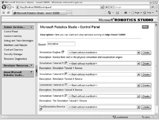
Each service is displayed with a drop-down box listing all of the manifests installed on the system that reference that service. You can run one of these manifests or you can start the service on its own. If you click the Create button next to Simulation Tutorial 1, the Control Panel will start that service and in turn start the SimulationEngine service.
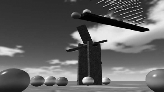
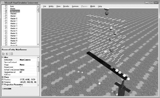
The controls for the simulator are fairly intuitive. The following sections explain the basics and provide some background information about how the simulator works. This section uses the ProMRDS.Marbles service to illustrate some of the simulator features. If you have installed the ProMRDS Package from the CD, you can start the service by typing the following in the MRDS command window: binMarbles.cmd. This file starts a DSS node and runs Marbles.manifest.xml. It should bring up the scene of the Marbles sample shown in Figure 5-3.
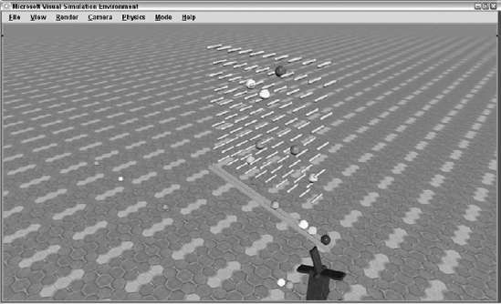
The Marbles sample doesn't actually do a lot of useful robotics-type things, but it helps to illustrate some of the simulator's features. In this sample, marbles are dropped from above and bounce through the grid of pegs until they roll down the ramp and hit the blades of the turnstile, causing the turnstile to turn. After 200 marbles have been dropped, instead of adding more marbles to the scene, the Marbles service picks them up from the ground and drops them.
When the simulator starts, it displays the simulated world as seen from the Main Camera. There is always a Main Camera object in the scene. Its position and orientation are often referred to as the eyepoint. Cameras are discussed in the section "The Camera Menu" later in this chapter.
Looking around in the simulator is very simple. Just press the left mouse button in the simulator window and drag the pointer around to change the viewpoint. This changes the direction in which the Main Camera is pointing.
You move yourself around in the simulator by pressing keys. It is easiest to navigate in the simulator with one hand on the keyboard and the other hand on the mouse. The following table shows the keys that move the eyepoint in the environment:
Key | Action |
|---|---|
W | Move forward |
S | Move backward |
A | Move to the left |
D | Move to the right |
Q | Move up |
E | Move down |
Notice that there are six keys and they work in pairs. W and S move you forward and backward. A and D move you left and right. Q and E move you up and down.
Holding down the Shift key while pressing one of the motion keys multiplies that motion by 10 times. This is very useful when you are in a hurry to get from one place to another. You can adjust the speed of mouse and keyboard movements in the Graphics Settings dialog, which is described shortly in the section "Graphics Settings."
The movements are always relative to the current eyepoint orientation. This enables you to combine key presses with mouse drags for more complicated motions. For example, you can press A to move to the left while simultaneously dragging the mouse pointer to the right to move in a circle around an object.
You can use the following function keys as shortcuts to commonly used functions:
Key | Action |
|---|---|
F2 | Change the render mode |
F3 | Toggle the physics engine on and off |
F5 | Toggle between edit mode and run mode |
F8 | Change the active camera |
Practice moving around in the environment until it becomes natural to you. Move yourself below the ground (that's right, there's nothing down there). Go as high as you can and see how the level of detail on the ground gradually fades into the fog. Practice zooming up to objects and moving right through them like a ghost. In the section "Physics Menu," you'll learn how to change the eyepoint so that it won't pass through objects.
Don't worry about getting lost in the simulator. If you ever wonder where you are, you can display the status bar (see Figure 5-4). Click View
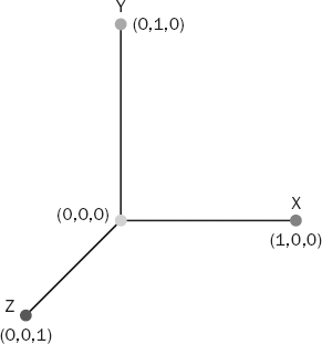
The status bar provides the position of the current camera, as well as the point that it is looking at. Every point in the simulation environment is represented by three coordinates: X, Y, and Z. The Y coordinate represents altitude, while the X and Z coordinates represent directions parallel to the ground plane. The simulation environment uses a right-handed coordinate system. This means that when the +X axis is pointing to the right and the +Y axis is pointing upward, the +Z axis is pointing out of the screen and the eyepoint is looking in the direction of the -Z axis (into the screen), as shown in Figure 5-5.
Also of interest on the status bar is the number of frames being processed per second and the number of seconds that have passed in simulation time since the simulator started.
You can click View
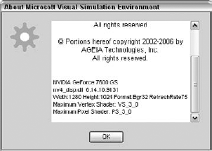
As you might expect, the Help menu gives you a couple of options to find out more about the simulator. The Help Contents option in the menu brings up the documentation file for the simulator. The second option, About Microsoft Visual Simulation Environment, can be used to display the version number of the simulator and specific information about your video card (see Figure 5-6):
The manufacturer and model
The name and version of the display driver
The size and format of the desktop
The highest supported versions of the vertex and pixel shaders
If your card supports version 3.0 of the shaders (VS_3_0 and PS_3_0) or higher, then you can display more realistic scenes, which include specular highlights and shadows.
Finally, here is your chance to be in two places at the same time. You can set up as many cameras in the simulation environment as you like and then instantly and easily switch between them, using the Camera menu. All cameras in the scene appear on the menu regardless of type. You can select the desired camera from the menu or you can press F8 to switch from one camera to the next. There are two types of behavior for cameras: real-time and non-real-time:
Real-time cameras: These render the environment from their viewpoint every frame. As you can imagine, multiple real-time cameras can increase the graphics load on a machine substantially. A real-time camera is appropriate when you have a need to retrieve images from that camera on a regular basis. Real-time cameras have a horizontal and vertical resolution associated with them. When the scene is rendered for that camera, it is rendered at that resolution.
Non-real-time cameras: These are simply placeholders in the 3D environment. Only the selected camera is rendered each frame. As a result, these cameras don't reduce graphics performance. They are useful when you want to define a viewpoint in the scene so that you can switch to it quickly. The Main Camera is a special instance of a non-real-time camera. There is always a Main Camera in the scene, and its resolution always matches the resolution of the display window. When the window changes, the Main Camera adjusts accordingly. Other non-real-time cameras have a set horizontal and vertical resolution. If the resolution of the display window doesn't match the resolution of the camera, the rendered image is stretched to fit.
The Marbles environment has several non-real-time cameras set up. Use the F8 key or the Camera menu to switch between them.
You've already seen how you can fly through the air faster than a speeding bullet in the simulator. You've seen how you can leap tall buildings in a single bound. (Okay, so we haven't had any buildings yet. Stay with us.) Now we'll give you X-ray vision.
The Rendering menu controls how the simulated world is displayed. Different rendering modes give you different information about how the world is put together. The following sections discuss the various modes.
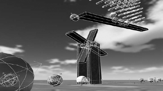
Shown in Figure 5-7, this is the default rendering mode, and you are already well acquainted with it. In this mode, the world is rendered to look its best—with fully rendered 3D meshes and lighting effects. This is the mode that you will probably use most often.
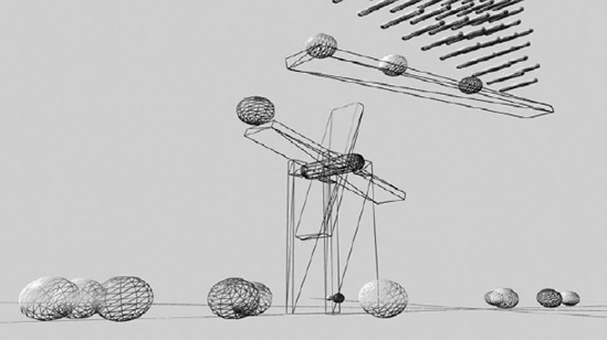
In this mode, shown in Figure 5-8, the world is still rendered with 3D meshes and lighting effects, but only the outline of each triangle is drawn. This quickly gives you a good idea whether the 3D meshes you are displaying have the proper resolution. Some meshes are so dense with polygons that they look about the same in wireframe mode as in the visual mode, which means they contain too many polygons and may be loading your graphics card more than necessary. Many modeling programs provide a way to reduce the number of polygons in a model.
Another benefit of wireframe rendering mode is that you can see through the objects in the scene. This is particularly helpful when you have just added a great new robot to your scene but it fails to appear. Switching over to wireframe mode shows that you accidentally embedded it in the couch.
The physics rendering mode (see Figure 5-9) shows you the physics shapes that make up the scene. This is the view that shows the physics shapes that the physics engine works with. Complex objects can sometimes be represented by very simple physics shapes such as boxes or spheres. The physics rendering mode enables you to see the scene the same way the physics engine sees it. If you notice that objects aren't colliding or moving the way you might expect, then switch to the physics rendering mode to see their underlying physics shapes.
It might be surprising but this mode can tax your graphics card more than the visual rendering mode even though less geometry is being drawn. This is because the shapes are composed of individual lines, which are drawn less efficiently than 3D meshes.
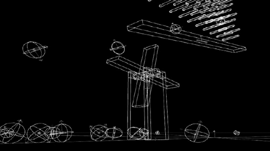
In Figure 5-9, you can see the three most common physics shapes: the sphere, the box, and the capsule. Spheres are defined by their radius. Boxes are defined by their dimensions along the X, Y, and Z axes. Capsules are cylinders with rounded ends, and they are defined by the radius of the cylinder and their height along the Y axis. Each of these shapes can also have a position offset and a rotation around each axis.
Notice in Figure 5-9 that each shape has coordinate axes drawn at its origin. You can deduce from the display that the origin of a sphere is its center. Although you can't see the color in the book, on the screen the X axis is drawn in red, the Y axis is green, and the Z axis is blue.
The simulation environment is composed of objects called entities, which typically represent a single rigid body such as a robot chassis that may contain multiple shapes. Each entity contains an optional 3D mesh and zero or more physics shapes. The visual representation of the object and the physics representation exist side-by-side. Entities are always positioned and rotated as a single object.
Entities are the basic building blocks of simulator scenes. The properties of the entities provided with the simulator are described in this chapter. Additional details about the implementation of entities are provided in Chapter 6.
In Figure 5-9, each entity has a cube that represents its center of mass. On the screen, the cube is red if the entity is controlled manually (kinematic), and white if the entity is controlled by the physics simulator. Each of the marbles in the scene is controlled by the physics engine; but the ramp and the mill supports have a red center-of-mass box, indicating that they are controlled by the program and not by the physics engine. All the pegs that the balls fall through are contained by a single entity, and you can see that this entity is kinematic by its red center-of-mass cube.
This mode (see Figure 5-10) combines the visual mode with the physics mode. In some cases, it is easier to see which outlines go with which shapes in this mode. The outlines of the physics shapes are drawn as if the visual rendering were transparent so that you can still see physics shapes that are obscured by other entities. This rendering mode will typically tax your graphics card the most, and you may notice the frame rate drop.
This is what your graphics scene looks like with the lens cover on the camera. At night. This mode is for those hardy souls who want to use the simulator completely for physics simulation and don't want to waste any time rendering. Turn the status bar on and select this rendering mode to see how many frames are processed per second. You'll learn how to use this mode a little later.
The last option on the Rendering menu takes you to the Graphics Setting dialog. These settings control how the graphics hardware is used to render the scene:
Exposure: This is much like the exposure on a camera. Increasing the exposure brightens the scene.
Anti-aliasing: This setting exposes the anti-aliasing modes supported by your graphics hardware. Selecting no anti-aliasing can make some cards run faster, but more anti-aliasing makes the edges of objects look much better. You have to experiment to find the best setting for your hardware.
Rotation and Translation Movement Scale: These numbers scale the movement for mouse and keyboard navigation. If you are one of those people who likes to turn your mouse movement up so high that you can zip across the screen with a millimeter of mouse movement, feel free to crank these values up.
Quality Level: Modern graphics hardware runs XNA shader programs to render objects. The simulator is equipped with version 3.0, 2.0, and 1.0 shaders. If you have newer and more powerful hardware, you can run version 3.0 shader programs and you will be rewarded with a nicer-looking scene and shiny specular highlights. If you have older hardware that only supports version 2.0 shaders, you will still get a nice-looking scene but it will lack specular highlights and some fog and lighting effects. The Quality Level option enables you to select which version of the shaders is used. The version that your card supports is marked as "Recommended" but you can switch between versions without any problem. A 2.0 shader card on one machine was able to run the 3.0 shaders, albeit a little slowly. (If you try this and your graphics card melts into a pool of glowing slag, forget that it was ever suggested.) If you find that your frame rate is lower than 10-20 frames per second, then try lowering the quality level to see whether it helps.
Just as there is a Graphics menu to control the way things look, there is also a Physics menu to control how things behave. The Physics Settings dialog is shown in Figure 5-11. You display it by clicking Physics
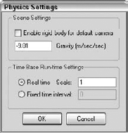
This dialog contains the following options:
Enable rigid body for default camera: This checkbox enables you to associate a physics sphere shape with the Main Camera. It is fine to observe what is going on in the simulation environment but sometimes you just have to poke or push something. If this option is checked, the camera can do just that.
You can try this out in the Marble environment by switching the render mode to physics mode. Enable the rigid body in the Physics Settings dialog and press OK. You should see a sphere appear just in front of the camera. You can verify that it works by maneuvering the camera down toward the turnstile, which is moved by the falling marbles. Position the camera on the opposite side of the turnstile from where the marbles are falling. Eventually you should be able to jam the mill and keep it from turning. Switch to the Mill View Camera and you should see a physics sphere shape blocking the mill from turning. This is the sphere shape associated with the camera.
Gravity: If you're planning to simulate the Mars Rover or the robot arm on the space shuttle, you'll want to use this setting to adjust gravity appropriately for your environment. The value is specified as a force along the Y axis, and it is negative because the Y axis is defined to go in the opposite direction as gravity. The gravity value is specified as meters per second, which works out to about −9.81 on Earth and −3.72 on Mars. If you're just aching to do it, go ahead and set it to a positive value. The gravity value is persisted as a part of the scene. When you load a previously saved scene, it will have the same gravity as when it was saved.
Time Base Run-time Settings: These settings control how simulator time is related to real time. They are the only settings on this dialog that are persisted from session to session independent of the scene that is currently loaded. To simulate the movement or collision of a robot with improved accuracy, you can slow down simulator time relative to real time. This causes the physics engine to process more steps per second, which improves accuracy. You can select a real-time scale of 0.1 to slow down the action in the simulator by 10 times. In this mode, simulator time is still related to the actual time that passes. You can select a fixed time interval (in seconds) to completely separate simulator time from real time. This is useful when you want to run a detailed physics simulation over a period of time and you aren't concerned with the graphics rendering during that time. You can choose a small fixed-time interval like 50 microseconds (0.00005) per frame and then set the rendering mode to No Rendering to increase the frame rate of the simulator to achieve a very accurate simulation. You can enable rendering periodically to see how the simulation is progressing.
You can turn off the physics engine by selecting the Enabled option on the Physics menu. If the physics engine is enabled, a check appears next to this menu option. When the physics engine is disabled, the simulator does not call the physics engine asking for scene updates. All dynamic entities stop moving but you can still move the camera around the scene. As far as the physics engine is concerned, no time passes, but the simulation time is still incremented on the status bar.
The physics rendering mode and the combined rendering mode are not supported while the physics engine is turned off. If either of these modes is selected when the physics engine is disabled, visual mode will be selected.
You can quickly toggle the physics engine between enabled and disabled by pressing F3. When the physics engine is disabled, the Physics Menu item on the Main menu bar is red.
You can disable the physics engine to temporarily freeze the scene. It is also useful to disable the physics engine while moving objects around in the scene with the Simulation Editor, as described in the "Simulation Editor" section coming up shortly.
A simulation scene can be saved or serialized to an XML file and reloaded later. When the scene is reloaded, the entities will have the same position and velocity as they had when the scene was saved. Click File
When a scene is saved, two files are actually written. The first contains the scene state and the .xml is appended to the specified filename. The second contains a manifest for the scene and it has .manifest.xml appended to the specified filename. This file is described in the next section.
Loading a scene is called deserialization. In order for it to be successful, all of the types referenced in the XML scene file must be currently defined in the CLR environment. If a type is not defined, the simulator will not be able to load that entity into the scene and it will display a warning dialog containing a list of all the entities that could not be instantiated.
If you run the SimulationTutorial2 manifest (or select Visual Simulation Environment Multiple Simulated Robots scene from the Start menu), a table and two robots will be displayed. The table is defined in the SimulationTutorial2 service. If you save this scene to a file, run Simulation Tutorial 1 (Basic Simulation Environment on the Start menu), and then attempt to load the previously saved scene, the simulator will complain that it is unable to instantiate the table because the service that defines the table is not loaded into the CLR. You can avoid this problem by running the SimulationTutorial2 service along with the SimulationTutorial1 service, adding code to SimulationTutorial1 to manually load the SimulationTutorial2 assembly, or by defining the table entity in a third DLL that is linked with both SimulationTutorial2 and SimulationTutorial1.
In a typical simulation scene, one or more services are associated with entities in the scene. Loading or saving a scene does nothing to start or stop services. For example, if you have a service that is driving your robot around at the time the scene is saved and then you reload the scene later, after the service has been terminated, that service will not be restarted.
The solution to this problem is the manifest. When a scene is saved, a manifest for the scene is also written to a file. This manifest contains service records for services that should be started. The manifest contains an entry for the SimulationEngine service, along with a state partner with the same filename as the scene file that was saved. In addition, it contains service records for other services that were associated with entities in the scene. Click File
The simulator has a built-in editor mode that makes it possible to modify or build a scene. Click Mode
When the editor starts, the physics engine is automatically disabled. The physics engine does not have to be disabled while the editor is running, but it is often much easier to work with entities in the scene if it is turned off.
While the editor is running, the display window is divided into three panes, as shown in Figure 5-12:
The main window renders the scene. When this window has input focus, it has a blue border around it and keystrokes affect the movement of the camera, just as in Run mode.
The upper-left pane, or the Entities pane, shows an alphabetical list of all the entities in the scene. Each entity has a checkbox next to it that selects it for various operations. If an entity has one or more child entities, a small box with a plus sign appears next to it. Clicking this box will show the child entities in the list.
The lower-left pane, or the Properties pane, shows all of the properties associated with the entity currently selected in the Entities pane.
Clicking the name of an entity highlights it and causes its properties to appear in the lower-left pane, the Properties pane. The Properties pane shows the name and type of the entity currently selected in the Entities pane. Below that, all of the properties of the selected entity are shown. Many of these properties can be modified.
When an entity is selected, it can be highlighted in the Display pane by pressing the Ctrl key. A highlighted circle is drawn around the entity that is not obscured by other entities (see Figure 5-13).
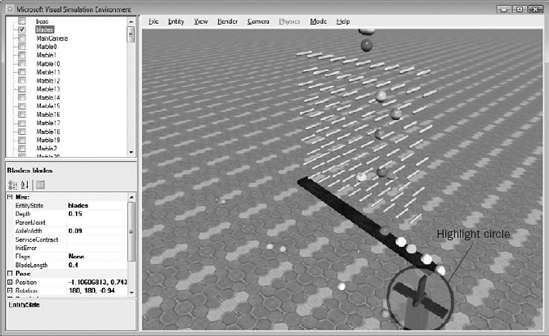
Another way to select an entity is to click with the right mouse button over the entity in the Display pane. The simulator determines which entities are under the position of the mouse click and selects the closest one. The ground and sky entities cannot be selected in this way.
It is very easy to identify each entity in the scene using this method. Hold down the Ctrl key so that the selected entity is highlighted and then right-click on various entities in the scene. The name of the entity and all of its properties appear in the Properties pane.
The Entities pane maintains two different entity selections. The entity that is highlighted in the Entities pane is the one that is shown in the Properties pane, and it is also highlighted in the Display pane. Entities can also be selected by clicking the checkbox by the name. It is possible to select multiple entities using the checkboxes, although only the highlighted entity is shown in the Properties pane. Operations that affect multiple entities will operate on all entities that are checked.
When an entity is selected, a number of additional operations are enabled on the entity. For example, it is a common problem to lose track of an entity and to be unable to see it in the scene. Sometimes the entity can be quickly located by selecting it in the Entities pane and then pressing the Ctrl key to highlight it. If the highlight cannot be seen, the eyepoint can be moved to the entity by holding down the Ctrl key and pressing one of the arrow keys, as described in the following table:
Key | Eyepoint Position |
|---|---|
Up Arrow | Above the entity (+Y) |
Shift + Up Arrow | Below the entity (−Y) |
Left Arrow | To the right of the entity (+X) |
Shift + Left Arrow | To the left of the entity (−X) |
Right Arrow | In front of the entity (+Z) |
Shift + Right Arrow | Behind the entity (−Z) |
You can move an entity around in the 3D environment by selecting its position property in the Properties pane. You can enter three values separated by commas to represent the new X, Y, and Z coordinates of the entity, or you can expand the position property and modify each coordinate separately.
Sometimes it is easier to position an entity graphically. To do this, select the position property and then hold down the Ctrl key to highlight the selected entity. Now press the left mouse button in the Display pane and drag the mouse pointer. The entity will move to follow the pointer. If you only want to move the entity along the X axis, simply select the X coordinate of the expanded position property, and when you drag the mouse pointer, the entity will only move along the X axis. The behavior is similar for the Y and Z coordinates.
The screen is only two-dimensional, so it is not really possible to move an entity in all three dimensions using the mouse pointer. The axes of movement are perpendicular to the vector formed by subtracting the camera Location from the camera LookAt point. You can move an entity parallel to the ground plane by positioning the camera directly above the entity looking down by pressing the Ctrl key and the up arrow and then dragging the mouse pointer with the left button held down.
You can rotate an entity in a similar way by selecting the rotation property of that entity and then dragging the mouse pointer while holding the Ctrl key. Selecting a single coordinate of the rotation property will constrain the rotation to be only around that axis.
Moving and rotating entities while the physics engine is enabled can be difficult. Gravity and other constraints in the environment can prevent or limit the movement of entities. You can disable the physics engine by pressing F3 or by toggling the Enabled item on the Physics menu, as described in the previous section.
You may have noticed that when you put the simulator in Edit mode, the Entities menu appears on the main menu. The items on this menu operate on one or more entities and are only available in Edit mode. The following sections briefly discuss each item on the menu.
You've already seen how to save and load an entire scene. It is also possible to save and load a subset of a scene. Entities can be
Sometimes it is more convenient to cut or copy and then paste selected entities. This is also done using the Entities menu. You can select one or more entities using the checkboxes in the Entities pane and then select either Cut or Copy from the Entities menu. At this point, the entities are serialized to a file called SimEditor.Paste in the Store directory. If you select Cut, the entities are deleted from the scene. When you click Entities
You can click Entities
Press OK when all of the selections are correct. The simulator will then display a dialog with properties for each parameter in the constructor of the new entity. When there are several constructors for an entity, the constructor defined immediately after the default constructor is selected. Press OK when all of the constructor parameters have been defined, and the entity will be created.
Occasionally, you must set some of the entity properties before you can successfully create the entity. For example, a SingleShapeEntity requires a shape to be defined but it cannot be specified in the constructor that is presented. The entity will appear in the Entities pane but it will have a red exclamation point next to it, indicating that there was an error in its creation. Look at the InitError property of the entity to see whether it provides some information about why the entity could not be initialized. In the case of the SingleShapeEntity, clicking one of the shape properties and defining a valid shape will clear the error, enabling the entity to be initialized.
The simulator supports the idea of child entities, which are entities that are defined relative to a parent entity. If you add a SingleShapeEntity as a child entity of another SingleShapeEntity, the child will be attached to the parent with a fixed joint that effectively glues the two pieces together. The physics engine treats the pair as if they were one entity.
When the simulator is in Edit mode, you can move and rotate the parent entity and the child entity moves with it. When you move or rotate the child entity, it changes the attachment of the child to the parent to accommodate the new position or rotation. This is how you can change the way in which the child is attached to the parent.
You can make one entity a child of another using the following steps:
Select the entity you want to make a child and press Ctrl1 to cut it from the scene.
Select the entity you want to be the parent.
Click Entity

You can also make an entity a child when you create it using the New Entity dialog described earlier by selecting the parent entity in the appropriate drop-down list.
Every entity in the simulation environment shares a common entity state. The entity state contains properties that affect the visual appearance of the entity as well as its physical behavior. Select an entity in the Entities pane. Its state is the property called EntityState, which has a value equal to the name of the entity. Click the value and an ellipsis (...) appears. When you click that ellipsis, a dialog box appears, enabling you to change the values of the entity state.
If you modify one or more entity state values and then select OK, the entity is removed from the scene and then reinitialized and inserted into the scene with the new values. This operation is similar to cutting the entity and then pasting it back into the scene.
The following sections discuss each part of the entity state.
Graphics assets determine how the entity looks. You can specify a new DefaultTexture, Effect, or Mesh to change the appearance of an entity:
DefaultTexture: If no mesh is specified for the entity, the mesh is generated from the physics shapes. In this case, the
DefaultTexturespecifies which texture map to apply to the generated meshes. The texture map should be a 2D texture and it can be any of the supported texture formats (.dds, .bmp, .png, .jpg, .tif).Effect: This is the shader program that should be used to render the entity. In most cases, you will just want to specify the default effect:
SimpleVisualizer.fx. Advanced users who want to create a special look for an entity can write their own shader program and specify it here.Mesh: If a mesh file is specified here, it is rendered for the entire entity. Only a single mesh file is supported per entity. As mentioned above, if no mesh is specified, then a default mesh is constructed from the physics shapes that make up the entity. Mesh files must be in .obj or .bos format.
The simulator reads .obj meshes. The .obj format (also called the Alias Wavefront format) is a popular 3D format that many modeling programs are able to export. These files usually have one or more material files with an extension of .mtl that specify the rendering characteristics of the objects. The format of .obj and .mtl files is ASCII, so they are easy to modify but less efficient to read, and large meshes can take some time to load. When an .obj file is read, the simulator automatically generates an optimized form of that file and writes it to disk with the same filename but with a .bos extension. The next time the .obj file is loaded, the simulator loads the .bos file instead, which is faster. If the obj file is modified, the simulator will not read the obsolete .bos file but will instead generate a new one. The MRDS SDK includes a command-line tool called Obj2Bos.exe, which can convert .obj files to .bos files without having to run the simulator. Microsoft has not made the .bos format public, so no tools outside of the simulator can read this format.
The following entity state properties appear under the Misc heading:
Flags: These bitwise flags define some physics behavior characteristics for the entity. If no flags are defined, then the default value for this field is
Dynamic, meaning the entity behaves as a normal dynamic entity, which is completely controlled by the physics engine. The other flags are as follows:Kinematic: If this flag is set, the entity is kinematic, meaning its position and orientation are controlled by a program external to the physics engine. The entity is not affected by gravity and it is not moved due to collisions with other objects, but it may influence the movement of other objects due to collisions.
IgnoreGravity: This one is self-explanatory. Gravity will have no effect on the entity if this flag is set.
DisableRotationX, DisableRotationY, DisableRotationZ: These flags prevent the entity from rotating around each of the specified axes. They are only relevant if the entity is not kinematic.
Name: This is the name of the entity. Each entity must have a unique name. Simulation services use the name of the entity to identify it, so it is important that no two entities have the same name. You can modify the name of an entity by changing it here, but any simulation services that previously connected to the entity will no longer work properly.
Velocity: This vector holds the magnitude and direction of the velocity of the entity. You can specify a new velocity in the state, and the entity will be updated with this new velocity. This state property is updated each frame, much like the
PositionandRotationproperties.
These properties in the entity state define physical characteristics of the entity:
AngularDamping/LinearDamping: These damping coefficients are numbers that range from zero to infinity. They provide a way to model real-world effects such as air friction, which tend to slow down the linear and angular motion of a body. The higher the number, the more the linear or angular motion slows. For example, entities with the default value of zero (0) for damping will continue to roll along the ground until some other force stops them.
Mass/Density: These properties are really two ways of specifying the same thing. If the mass is nonzero for one or more of the physics shapes in an entity, the physics engine will calculate the total mass and density of the entity from the sum of the mass of the shapes. In this case, these two values are ignored when the entity is initialized. If the sum of the masses of the shapes is zero, then the physics engine uses one of these values to determine the mass of the entity. The
Massvalue provides a shortcut for specifying the total mass of an entity. The physics engine calculates the center of mass assuming that the density of the shapes in the entity is uniform. TheDensityvalue provides another shortcut to specify the overall mass. IfDensityis specified, the physics engine calculates the total mass based on the volume of the shapes in the entity. Again, the engine assumes that the density is uniform throughout the entity.InertiaTensor: This property is a way to specify the mass distribution of the entity. The inertia tensor expresses how hard it is to rotate the shape in various directions. Shapes such as cylinders are naturally easier to rotate around their longitudinal axis but more difficult to rotate around the other two axes due to their mass distribution. If this vector is not specified, the physics engine will calculate it based on the position and relative size of the shapes in the entity.
The following properties are common to all entities. Just like the other entity state, they can be edited in the Properties pane of the Simulation Editor.
ServiceContract: This property is an optional URI for a service that controls or interacts with this entity. When the scene is saved and a manifest is written, the simulator will add this service to the list of services that run and specify the name of this entity as a partner.
InitError: If an entity fails to initialize, it is displayed in the Entities pane with a red exclamation point. When this happens, the error displays in the
InitErrorproperty.Flags: These are miscellaneous bitwise flags that apply to the entire entity:
UsesAlphaBlending: Set this flag if your entity is partly transparent. The simulator renders transparent entities last.
DisableRendering: Set this flag to skip rendering of this entity. This is very useful for entities that are large and cover up other entities. Even though the entity is not drawn, it still is active in the scene.
InitializedWithState: This flag is supposed to indicate that the entity was deserialized from a file, rather than built with a nondefault constructor. The simulator does not appear to set or pay attention to this flag currently.
DoCompletePhysicsShapeUpdate: This flag specifies that the physics engine should update the pose information for each physics shape in the entity each frame. By default, the shape state is not updated each frame.
Ground: This flag indicates that the entity is the ground. This flag is set by some entities but the simulator does not currently do anything with it.
ParentJoint: This is the joint that connects a child entity to its parent. It is discussed in more detail in Chapter 8 when we get to articulated entities.
Position and Rotation: These properties were previously discussed in the section "Misc" earlier in the chapter. Together they specify the position and orientation of the entity in the environment.
MeshScale/MeshTranslation/MeshRotation: These properties make it easier to fit a 3D mesh to an entity. Because different modeling tools have different defaults for axis orientation and scale, it is sometimes difficult to export a model that exactly matches an entity in the simulation environment. Perhaps the mesh is rotated by 90 degrees or perhaps the modeling package uses centimeters rather than meters. These properties make it easy to scale, move, and rotate the mesh so that it fits the physics shapes that define the entity.
Meshes: This property shows information about the meshes that are loaded for the entity. These meshes may have been constructed from the physics shapes that make up the entity, or they may have been loaded from a .obj file. There is not much you can change about the meshes, but you can change the materials that go with the meshes. This is a great way to tune the appearance of entities within the environment. You can make them darker or lighter, or you can change how shiny they look. The color of an object in the simulator is a combination of ambient, diffuse, and specular light. The simulator uses a high–dynamic range lighting model, so it is fine if these values sum to a color greater than (1,1,1). At the end of all the lighting calculations, the color of the object is clamped to the range that the graphics hardware can display.
It is easy to tune the way objects look in the environment by modifying the following material properties. The material properties are part of the entity state, but they are usually set when a mesh is loaded because they describe the appearance of the mesh. For example, a .obj mesh file usually has an associated .mtl material file that defines the material properties for each mesh. If you change the material properties using the Simulation Editor and you want those changes to persist between sessions, then you must tell the simulator to save the material changes back to the source files. To do so, click File
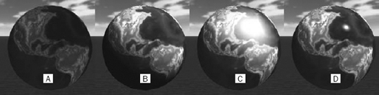
Ambient: This color value determines how much light is reflected from the object due to ambient light, which is light that is scattered throughout the environment from other objects (see Figure 5-14a). Typical values for the color components of the ambient color range from 0 to 0.2.
Diffuse: This color value determines how much light is reflected from an object due to being lit by a diffuse light (see Figure 5-14b). This value represents the maximum amount of light that will be reflected for the part of an object that faces directly toward the light. Parts of the object that are more edge-on to the light are lit less by that light, and parts of the object that are perpendicular to the light are not lit at all. Diffuse lighting is what gives a 3D look to shapes in the environment because the amount of light that is reflected depends on the orientation of the shape with respect to the light. Values for diffuse color typically range between 0.4 and 0.8.
Specular: This color value determines how much light is reflected from an object in a specular highlight (see Figures 5-14c and d), which is basically a hack to make an object look shiny, as if it were reflecting the actual shape and color of the light. The specular highlight color is typically the same color as the light, whereas the diffuse color is typically the color of the object.
Power: This value determines the "tightness" of the specular highlight. The higher the power, the smaller the highlight. Figure 5-14c shows a specular highlight power of 2, whereas Figure 5-14d shows a specular highlight power of 128. Typical values range from 32 to 256.
The simulator exists to provide a way for you to create your own robots and environments. The Simulation Editor discussed in the previous section enables you to compose and modify environments using the built-in entities that are provided with the simulator. The following sections go into more detail about these entities. The next chapter describes how you can define your own custom entities.
In the following sections, the built-in entities have been divided into four categories:
Sky and ground entities
Light entities
General-purpose entities
Robot and sensor entities
Only wheeled robot entities are discussed in this chapter. Jointed entities, such as arms and walkers, are discussed in Chapter 8.
All of the 3D meshes and textures used by these entities can be found in Store Media. When you add your own media files, you should place them there as well.
The simulator provides two built-in entities to define the sky, as well as a number of entities to define various types of terrain. You can build a scene without these entities if you prefer, but they make the environment look more realistic, particularly for outdoor scenes.
You don't really pay a lot of attention to the sky until there isn't one. The sky provides diffuse scattered light that illuminates objects in the scene. It is also sometimes useful to simulate bright and overcast outdoor conditions. The difference between the Sky entity (see Figure 5-15a) and the SkyDome entity (see Figure 5-15b) is the way they are drawn:
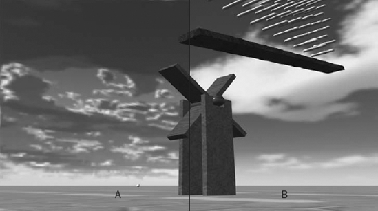
The
Skyentity surrounds the entire scene with a 3D sphere mesh. A cube map, specified in theVisualTextureproperty of theSkyentity, provides the color of the mesh. This method of drawing the sky is somewhat inefficient because the ground obscures half the sky mesh that is drawn. Half the texture stored in memory is never seen. The texture used by the simulation tutorials for the sky is simply calledSky.dds.The
SkyDomeentity is more efficient because it uses a half dome to surround only the part of the environment above the ground. It is colored by a 2D texture map such asSkydome.dds. The one disadvantage to theSkydomeentity is that if you rise too high in altitude, you may see a gap between the sky and the ground. TheSkyentity is preferable for high-altitude simulations.
Both the Sky entity and the SkyDome entity can add to the diffuse lighting of the scene. The color and intensity of light that they cast on the entities in the scene is defined by a special texture map called a cube map. To visualize how a cube map works, imagine yourself on the inside of a giant cube. Each of the six faces of the cube has an image on it so no matter which direction you look, you see a pixel in one of the images. The lighting cube map surrounds the entire scene and defines the color and intensity of the light that shines on the entities from each direction. It is common to define a diffuse light map that lights entities brightly from above and less from the sides. The illumination coming from below is usually a little more than from the sides to simulate light scattering from the ground.
You can see how this cube map affects the lighting of the scene by clicking Start
The Sky and SkyDome entities also provide a way to set the fog in the scene. The FogColor property defines the color of the fog. For a night scene, you want to use black fog, and for a day scene, grayish or white fog. Using the FogStart property, you can also specify the distance at which fog begins to appear. The FogEnd property specifies the distance at which entities in the scene are completely fogged. The fog increases linearly between the FogStart distance and the FogEnd distance.
One diffuse sky texture is provided with the MRDS kit. It is called, oddly enough, sky_diff.dds. The .dds format is associated with DirectX, and the extension was originally an abbreviation for Direct Draw Surface. These days, .dds files are most often used as texture maps for Direct3D. You can edit and create .dds texture maps using the DirectX Texture Tool, which is part of the DirectX SDK described previously in this chapter under the section "Software Requirements."
The simulator changes the Y offset of the Sky and Skydome entities to follow the eyepoint of the Main Camera. This prevents the camera from ever going above the sky. Do you remember that episode of Star Trek in which a whole colony of people were living inside a hollowed-out asteroid that was a spaceship, except they didn't know it was a spaceship until an old guy climbed a mountain and touched the sky? You don't have to worry about that in the simulation environment.
The
SkyDomeentity is used in Simulation Tutorial 1. You can run this environment by clicking Start
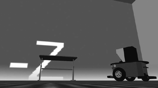
If you find yourself occasionally becoming disoriented in the simulation environment, you can literally paint a compass in the sky using the Sky entity. Start the Simulation Editor by pressing F5 and then select the Sky entity. In the VisualTexture property, select Directions.dds. This texture will paint the direction you are facing on the sky (see Figure 5-16). For example, if you are looking along the +Z axis, then you should see +Z ahead of you.
The HeightFieldEntity is used as a ground plane in many of the simulation tutorials provided with the SDK. It is one of the more important components in the scene because without it, everything falls into an abyss.
A HeightFieldEntity is flat, with an elevation of 0 meters. It may seem infinitely large but it is really just 49,000 square meters, ranging from (−4000, 0, −4000) to (3000, 0, 3000). Columbus would not have fared well in the simulation environment.
A HeightField shape contains a grid of height values. The HeightFieldEntity uses a grid of 8 rows by 8 columns, and it sets the altitude of each height value to 0.
The most remarkable feature of the HeightFieldEntity is the texture that is applied to it. The default texture used in most of the SDK samples is 03RamieSc.dds, which looks a little like industrial carpet. It is a little depressing to look at 49,000 square meters of carpet, so you are encouraged to find another texture for your scenes. The only requirement is that the texture should tile properly without any seams, because it is repeated across the ground many times. The default scaling for the texture on the ground plane is 1 meter by 1 meter. This scale can be changed programmatically but it can't be changed using the Simulation Editor.
You can change the texture associated with the ground by selecting the ground and then opening its
EntityStateproperty. Enter a new 2D texture filename in theDefaultTextureproperty.
The friction and restitution (or bounciness) of the ground can be changed by editing the HeightFieldShape property. This brings up a dialog that enables you to edit its shape properties, among which are StaticFriction, DynamicFriction, and Restitution. These shape properties are described more fully in the upcoming section, which describes SingleShapeEntities.
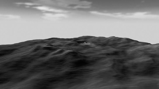
The TerrainEntity is a much more interesting way to describe the ground than the HeightFieldEntity. The HeightFieldEntity is fine for simulating indoor scenes, but the challenge that many robots face is navigating uneven ground in an outdoor environment. The TerrainEntity provides a way to construct such an environment.
You can take a look at a TerrainEntity by clicking Start
There aren't many TerrainEntity properties that you can modify in the Simulation Editor, but you can change the image that generates the HeightField and the texture that you apply to it. Start the Simulation Editor by pressing F5 and select the entity named Terrain. Change TerrainFileName to another image filename, such as particle.bmp. Nothing immediately happens because this particular entity does not automatically refresh when a property is changed. With the TerrainEntity still selected, press Ctrl+X and then Ctrl+V to refresh the terrain. You'll notice that the ground level has changed noticeably, and when you leave the Simulation Editor by pressing F5, the physics engine will pop the buried objects out of the ground.
You can change the texture that is applied to the TerrainEntity by changing the DefaultTexture in the EntityState property.
The TerrainLODEntity is identical to the TerrainEntity except that it does some extra tricks to try to reduce the load on the graphics system. It calculates a reduced resolution version of each section of the height field and then uses that version when the section is far away from the eyepoint. This reduces the number of triangles that must be drawn, as shown in Figure 5-18. The left side of the figure (a) shows the TerrainEntity and the right side (b) shows the TerrainEntityLOD. It does not reduce the number of HeightField samples used by the physics engine, so it does not affect physics behavior.
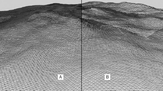
Unfortunately, the TerrainEntityLOD may not be suitable for many applications because it changes the height values for portions of the terrain in the distance, which may cause some entities to be incorrectly visible or obscured in the distance. In addition, it makes no attempt to seam together the edges of each section, so you may see unattractive cracks between sections. Nonetheless, if your graphics card is struggling to render a scene with terrain, the TerrainEntityLOD is an option for you.
The simulator provides three different types of lights to illuminate the scene. They are implemented as a single LightEntity, which has three different modes of operation, described further in this section. You can define up to three lights in the scene, but be aware that each additional light creates extra work for the graphics chip and may reduce your frame rate. You can continue to use the simulation environment with Terrain to see how lights work in the simulator.
You use a directional light to model a light that is very far away, such as the sun. The position of the light doesn't matter, only its direction. Most of the tutorial and sample scenes provided with the SDK include a directional light named Sun. Put the simulator into Edit mode by pressing F5 and select the Sun entity. Now select its Rotation property and drag the left mouse button while holding the Ctrl key to see how changing the direction of the light affects the lighting in the scene.
When the simulator is in Edit mode, LightEntities are represented by simple meshes, as shown in Figure 5-19 (from left to right, directional lights, omni lights, and spot lights).
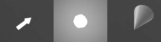
The Color property defines the color of the light for all light types. The SpotUmbra, FalloffEnd, and FalloffStart properties do not affect directional lights.
Omni lights are so named because they send light out in every direction. Consider light bulbs. These lights are usually very close to the objects that they illuminate, so their position is very important; but because they cast light in every direction, their rotation is unimportant.
You can change the Sun to be an omni light by changing its Type property. Try changing its rotation just as you did for the directional light. No effect. Now select its Position property and move the light around. You can see that even small changes in the position of the light change the way entities are lit in the scene.
If you ever need to position a light in the scene but you can't find it, you can use the same trick that works for every other entity. Select it in the Entities pane and then hold the Crtl key and press the up arrow. The eyepoint will be moved to be just above the selected light.
The FalloffStart and FalloffEnd properties affect both omni lights and spot lights. They define the distance at which the light starts to diminish and the distance after which the light has no effect, respectively. Unlike the sun, light bulbs tend to have limited range here on earth.
Finally, a light for which position and rotation are both important. In the real world, many light bulbs have reflectors and shades to direct the light in a particular direction. That is exactly what a spot light does. It projects a cone of light with the apex at its position. The angle swept out by the cone is specified by the SpotUmbra property. These types of lights are good for headlights or emphasis lights.
Light shadows provide cues to our brain regarding the position of objects in the world. They can be a help to robot vision processing algorithms and they can also be an added challenge. The simulator supports casting shadows from one light. Each LightEntity has a CastsShadows property, which, when set to True, causes that light to cast shadows. Switch the Sun back to an omni light and turn on shadows. The first time shadows are turned on, the simulator must generate special shadow meshes for each mesh in the scene. If a mesh was read from a file, the shadow mesh is saved to a file in the storemedia directory with the same name as the mesh file but with a .shadowMesh.bin extension. It may take several seconds to generate shadow meshes for very complex or large models. For example, the LEGO Tribot can take 20–30 seconds on a fast machine. The next time the shadow meshes are needed, they are read from the disk, rather than generated. If the original mesh is changed, its shadow mesh is updated.
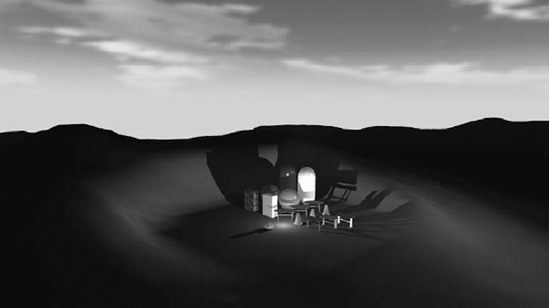
Move the omni light around the scene and note how the shadows are updated (Figure 5-20 shows shadows cast from a single omni light). The entities in the scene are self-shadowing, which means that one part of an entity can cast a shadow on another part.
If more than one light has the CastsShadows property set to True, the simulator will cast shadows from the first light encountered as it is drawing the scene. Be aware that drawing shadows is expensive and can slow down the rendering of the scene substantially.
Some entities in the environment don't justify extensive modeling. If you need to test how well your robot avoids obstacles, a few entities made of a single box shape will probably suffice. You can build furniture or stairs or ramps out of multiple box shapes.
The simulator provides the SingleShapeEntity, the MultiShapeEntity, the SimplifiedConvexMeshEnvironmentEntity, and the TriangleMeshEnvironmentEntity to make it easier for you to add objects to your scene. Each of these entities is used in the scene built by Simulation Tutorial 5 and is discussed in detail in this section. You can run this scene by clicking Visual Simulation Environment
As the name implies, this entity is wrapped around a single physics shape—either a sphere, a box, or a capsule. This is the easiest way to add a single object to the environment: Decide which shape will best represent the object, specify its dimensions, and add it to the scene. You can even specify a mesh to make it look more like the object you are modeling.
The bluesphere, the goldenscapsule, and the greybox are good examples of SingleShape entities that use the various physics shapes. In the Simulation Editor, you'll notice that SingleShape entities have three properties under the Shape category representing each of the three possible shapes. You can edit the properties for the shape that is defined, or you can click the value of one of the other shape properties to change the entity to use that shape. This is probably a good time to talk about general shape properties because they are used in nearly every entity.
Expand the shape properties associated with the sphere in the bluesphere entity. The properties are divided into the following categories: MassDensity, Material, Misc, and Pose. The Material category is where the friction and restitution properties of the shape are specified. Several shapes may share the same material, and changing the material for one shape will affect the other shapes as well.
Misc | |
|---|---|
Each shape has a default color that is used to create a visual mesh if no other mesh is specified in the | |
| A box shape uses all three dimensions to specify its size along each axis. The sphere shape uses only the |
Shapes can be set to provide a notification when they contact another shape. This option is not very useful in the Simulation Editor but it can be very useful when writing a service. For more on services, see Chapters 2, 3, and 4. | |
| It is not necessary to set the name but it can be useful when the shape is passed to a notification function and you need to identify which entity it is part of. |
This identifies the type of the shape. | |
Like | |
| This specifies the offset and orientation of the shape compared to the origin of the entity. This becomes more important in the |
Several of the entities in the terrain scene do not specify a 3D mesh, so their visual mesh is built from the shape itself. The StreetCone entity does specify a 3D mesh. Switch to the combined view and look at this entity, and you will see that it is just a single cube for physics purposes but looks like a traffic conevisually.
The MultiShapeEntity is much like the SingleShapeEntity except that it contains—yes, you guessed it—multiple shapes. It only supports boxes and spheres but you can have as many of them as you like. The table_mesh entity in the scene is built from multiple box shapes, but you would never know it until you select the physics view because it also uses a 3D mesh to give it a nicer visual appearance.
The state for a MultiShapeEntity is very similar to the state for a SingleShapeEntity except that the BoxShapes property is a collection of boxes and the SphereShapes property is a collection of spheres.
This entity enjoys the distinction of having the most syllables of any other built-in entity so it must be important. In some cases, it is not sufficient to have a single box represent the physical shape of an object because it just doesn't collide with other objects the right way. The simulator can construct a physics object called a simplified convex mesh from any 3D mesh. A convex mesh is built from the points of a convex hull, which is the smallest polyhedron containing all of the points of the original mesh. You can think of generating a simplified convex mesh as similar to taking an arbitrary mesh and wrapping it with shrink wrap. When you heat the shrink wrap and it pulls tightly around the object, the resulting shape is very close to the convex mesh representation. (Of course, the physics SDK does this using math, not shrink wrap.)
SimplifiedConvexMeshEnvironmentEntities interact with the physics environment just like spheres, boxes, and capsules except that they are more expensive to calculate. The table_phys_m is an example of this type of entity. It is shown in Figure 5-21 (right) along with a TriangleMeshEnvironmentEntity (left).
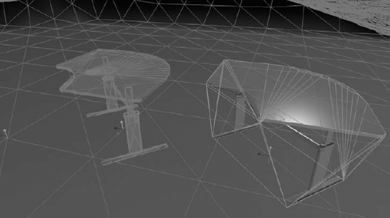
The state associated with a SimplifiedConvexMeshEnvironmentEntity is very similar to the other entities except that it must have a 3D mesh specified in the EntityState. This is the mesh that will be used to construct the convex mesh. The maximum number of polygons in the simplified convex mesh is 256.
This entity is very similar to the SimplifiedConvexMeshEnvironmentEntity except that the entire 3D mesh is used for the physics shape instead of constructing a convex mesh. Because the physics shape is identical to the visual shape, the entity will collide and move just like the visual shape.
You may be tempted to use a TriangleMeshEnvironmentEntity for every object in the scene, but you should be aware that this type of entity has some limitations. Collision detection is not as robust as it is for other shapes. If a shape moves fast enough that its center is inside the triangle mesh shape, then a collision may not be registered. In addition, SimplifiedConvexMeshEnvironmentEntities must be static entities, meaning they cannot be moved around in the environment, and they act as if they have infinite mass.
Let's see, what was this book about again? Oh yeah, robots! We should talk about some robots. This chapter covers simulating differential drive robots. In Chapter 8, you'll look at robots with joints. A differential drive consists of two wheels with independent motors. A differential drive robot can drive forward or backward by driving both wheels in the same direction, and it turns left or right by driving the wheels in opposite directions. Usually, one or two other wheels or castors provide stability.
In this section, you will learn how to drive the iRobot Create, the LEGO NXT, and the Pioneer 3DX robots in the simulation environment. Each of these robots is based on the DifferentialDriveEntity. You'll also learn how to use sensors such as bumpers, laser range finders, and cameras.
The best way to become familiar with differential drive robots is to drive one around. Click Start
SimulationEngine: This is the simulator and it has a state partner that causes the simulator to load its initial scene from the file
iRobot.Create.Simulation.xml.SimulatedDifferentialDrive: This service connects with the iRobot Create entity in the simulation environment and then drives each of its motors according to the commands that it receives.
SimulatedBumper: This service sends a notification to other services when the bumpers on the iRobot Create make contact with another object.
SimpleDashboard: This service provides a Windows Forms user interface that can be used to send commands to the DifferentialDrive service to drive the robot.
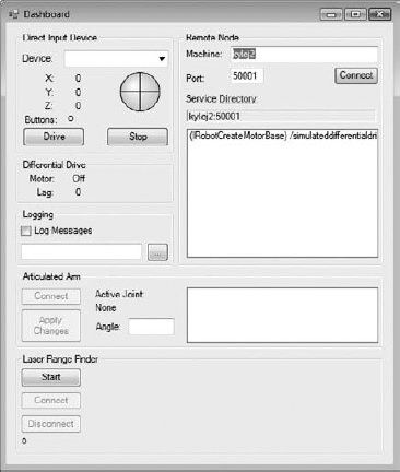
Follow these steps to connect the dashboard to the differential drive service and drive the iRobot Create in the environment:
Type your machine name in the Machine textbox. Alternatively, you can just type localhost to select the current machine.
Click the Connect button. The (IRobotCreateMotorBase)/simulateddifferentialdrive service should appear in the list labeled Service Directory.
Double-click the (IRobotCreateMotorBase) /simulateddifferentialdrive/ entry. The Motor label should change to On in the Differential Drive group box.
Click the Drive button in the Direct Input Device group box to enable the drive control. Don't forget this step!
Drag the trackball graphic forward, backward, to the left, and to the right, to drive the robot in the environment. Go wild. Crash into entities to your heart's content and take satisfaction in knowing that no one will present you with a bill for a damaged blue sphere.
You can also drive simulated robots and actual robots using a wired Xbox 360 controller. Plug the controller into an open USB port. You will be able to drive the robot using the left thumbstick. If you are using the simulator, you can also move the camera around the environment using the right thumbstick. The only downside is that it's hard to convince your colleagues that you are doing serious robotics work while holding an Xbox 360 controller.
The LEGO NXT Tribot is the first robot you build with the LEGO NXT kit. It has two drive wheels and a castor in the back. It also has a number of sensors that you can mount to the robot, but the one in the simulation model is the touch sensor, or bumper. You can run an environment that contains a LEGO NXT Tribot, a Pioneer 3DX robot, and a lovely table by selecting Visual Simulation Environment Multiple Simulated Robots.
When you connect the Dashboard, you'll see three services. You can drive the Tribot by double-clicking the (LEGONXTMotorBase)/simulateddifferentialdrive/ service. This is the service that is used with all three differential drive robots in the simulator. It provides a connection between the DifferentialDriveEntity in the simulator and services outside the simulator. When you examine the ServiceContract property of the LEGO NXT Tribot, you will notice that it references the contract ID for the SimulatedDifferentialDrive service.
Put the simulator into Edit mode by pressing F5. You'll notice that the Physics menu turns red, indicating that the physics engine has been disabled. You'll also notice that you can no longer drive the robot. When you can't drive a robot in the simulation, ensure that the physics engine is enabled.
The LEGONXTMotorBase entity in the Entities pane has a single child entity, LEGONXTBumpers, which is a BumperArrayEntity. This entity has an array of box shapes that define where the bumpers are located. The LEGO NXT Tribot uses only a single box shape. The ServiceContract property of the LEGONXTBumpers entity is set to the contract identifier for the SimulatedBumper service. This service connects with the BumperArrayEntity and provides a way for other services to be notified when the bumpers are in contact with another shape.
The iRobot Create, the LEGO NXT Tribot, and the Pioneer 3DX entities all inherit from the DifferentialDriveEntity. This is what enables the SimulatedDifferentialDrive service to work with all three of them. Most of the properties of the DifferentialDriveEntity can only be set programmatically, but a few are useful in the Simulation Editor:
CurrentHeading: This is a read-only property that indicates the current heading of the robot in radians. The heading is 0 when the robot faces along the -Z axis and it increases as the robot turns left.
MotorTorqueScaling: This factor multiplies the torque applied to the wheels when
SetMotorTorqueis called.IsEnabled: This is
Trueif the drive is enabled.
Not all robots in the simulation environment need to inherit from the DifferentialDriveEntity. It simply serves as a convenient way to provide common services and properties for two-wheeled differential drive robots. You'll learn how to implement more complicated robots in the next chapter.
The Pioneer 3DX Robot is manufactured by Mobile Robots, Inc. It is interesting because it has an onboard laser range finder and an onboard computer, so it is capable of autonomous movement. It also has bumpers, and the version in the simulator has a mounted webcam.
You've already learned about cameras in the scene but this camera is mounted to the robot as a child entity. When an entity is added as a child of another entity, its position and orientation are relative to the position and orientation of the parent. When the parent moves, the child moves with it. Adding a CameraEntity as a child entity of the Pioneer3DX entity causes the camera and its image to follow the robot.
Try this out by double-clicking the (P3DMotorBase)/simulateddifferentialdrive/service in the
Servicedirectory list of the Dashboard. Click the Drive button to enable the drive and verify that you can drive the Pioneer by dragging the trackball icon. Now switch the simulator view to the camera mounted to the Pioneer by selecting robocam from the Camera menu. Drive the robot around and you will see what the robot sees.
The ServiceContract property of the robocam entity shows that it is associated with the SimulatedWebcam service. This service reads the images generated by the real-time camera and makes them available to other services or to users via a browser window. You can watch updated images from any real-time camera in the scene in a browser window by following these steps:
Make sure the Visual Simulation Environment
Open a browser window and point it to
http://localhost:50000. The image from the SimulatedWebcam service appears in a browser window (see Figure 5-23).Click either service that begins with /simulatedwebcam/.
Select a refresh interval and click Start. The web page should periodically update with a new image from the camera.
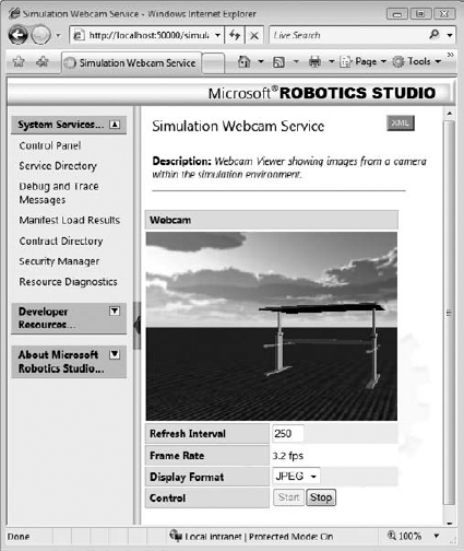
A laser range finder is a sophisticated and expensive device for measuring distance. It uses a laser to sweep a horizontal line in front of the robot. The laser measures the distance to objects in front of the robot by shining a low-power laser and then recording the light that is bounced off of objects. As the laser sweeps in a horizontal arc, the number of samples that it takes defines its angular resolution.
The LaserRangeFinderEntity simulates a laser range finder by casting rays into the simulation environment that correspond to laser samples. These rays are intersected with the physics shapes in the environment, and an array of distances is returned. Small, flashing, red circles are drawn in the environment at each intersection point. You may notice that these hit points are sometimes drawn in mid-air where no object is visible. This is usually because the physics shape that represents an entity is different from the visual mesh that represents the entity. This is the case with the table in the scene. Switching to combined rendering mode shows that the box shapes defining the sides of the table are quite different from the visual mesh of the table. The laser always operates on physics shapes.
The Dashboard user interface provides a way to visualize the laser range finder data. Follow these steps to enable this feature:
Click Start
Connect the Dashboard by entering the computer name or localhost in the Machine textbox.
Double-click the (P3DXLaserRangeFinder)/simulatedlrf service in the Service Directory list.
An image of two box shapes should appear in the Laser Range Finder window at the bottom of the dialog. Darker pixel colors represent objects that are nearer to the robot.
This chapter has been a user guide to the simulator. The functionality provided by the simulator has been explained and the built-in entities have been described. Several example scenes have been demonstrated. You might want to remember the following key points as you head into other chapters:
The Microsoft Robotics Developer Studio Visual Simulation Environment is a 3D virtual environment with a powerful physics engine. It can be used to prototype algorithms and new robot designs.
The simulator provides a user interface to move through the environment, as well as to change the rendering mode and save and restore scenes.
The simulator has a built-in editor that enables entire scenes to be defined. Robots and other entities can be created and placed in the environment.
The simulator provides several built-in entities, including robots and sensors.
Custom entities can be defined and used in the environment.
The environments and robots provided with the SDK are interesting, but the real utility and fun comes from building something new. That is what is covered in the next four chapters, where you will learn about adding new entities and simulation services and creating new environments.