
Chapter 4 introduced some of the basic modeling techniques required when creating a 3D parametric part. Modern parametric modeling utilizes numerous tools to create stable, editable parts. The basic workflow of creating a part is to create a base feature and then build upon that base. The tools used to build the additional features can vary depending upon your need and may range from simple extruded features to complex combinations of different feature types.
In this chapter, you will be exploring some of the more complex and curvy modeling techniques. Some of these features involve creating a base profile sketch along with support sketches used for defining paths and shape contours. Such features are based on the same rules used to create simpler features, such as extrudes and revolves, but they take it to the next level by using multiple sketches to define the feature. Other advanced features covered in this chapter depart from these concepts and move into new territory of feature creation. In either case, having a strong understanding of sketch creation and editing principles is assumed and recommended.
All the skills in this chapter are primarily based on creating a single part, whether in a part file or in the context of an assembly file.
In this chapter, you'll learn to:
Now that you have moved on from creating simple features, you can explore the use of sweeps and lofts to create features of a bit more complexity. Both sweeps and lofts require one or more profiles to create a flowing shape. Sweeps require one sketch profile and a second sketched sweep path to create 3D geometry. Lofts require two or more sketch profiles and optional rails and/or points that assist in controlling the final geometry.
You can think of a sweep feature as an extrusion that follows a path defined by another sketch. 2D or 3D sketch paths can be used to create a sweep feature. As with most Inventor geometry, a sweep can be created as a solid or a surface. You should note that sweeps can add or remove material from a part, or you can use the Intersect option as you can with the Extrusion command. If your intent is to create multi-body parts, then you can choose the New Solids option also.
When creating a sweep feature, you will typically want to first create the path sketch and then create a profile sketch that will contain the geometry to be swept along the path. To create the profile sketch, you will need to create a work plane at the end of your path. This work plane will be referenced to create a new sketch. It's not mandatory that you create the path and then the profile, but it is easier to define the profile sketch plane (that is, a work plane) by doing it this way. Normally, this geometry will be perpendicular to one end of the sweep path.
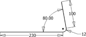
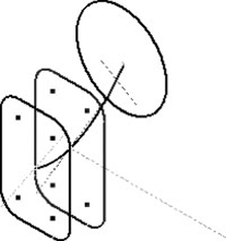
A basic rule of sweep features is that the volume occupied by the sweep profile may not intersect itself within the feature. Self-intersecting features are not currently supported. An example of a self-intersecting feature is a sweep path composed of straight-line segments with tight radius arcs between the segments. Assuming that the sweep profile is circular in nature with a radius value larger than the smallest arc within the sweep path, the feature will self-intersect, and the operation will fail. For a sweep to work, the minimum path radius must be larger than the profile radius. In the 2D sketch path example shown in Figure 5.1, the path radius is set at 12mm. Knowing that the minimum path radius value is 12mm, you can determine that the sketch profile radius must be less than or equal to this value.
Once a sketch path has been created, you can create a work plane on the path and then sketch the profile on that plane. To see this process in action, follow these steps starting with the creation of the path:
On the Get Started tab, click the New button.
On the Metric tab of the New File dialog box, select the
Standard(mm).ipttemplate.Create a 2D sketch as shown in Figure 5.1.
Once you've created the sketch path, right-click and choose Finish Sketch; then click the Plane button on the Model tab to create a work plane.
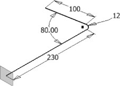
Select the endpoint of the 2D sketch path and then the path itself to create the plane. This creates a plane on the point normal to the selected line. Figure 5.2 shows the created work plane.
Once you've created the work plane, right-click the edge of it, and select New Sketch.
In the new sketch, use the Project Geometry command to project the 230mm line into this new sketch. It should come in as a projected point.
Next, create a circle anchored to the projected point, and give it a value of 20mm in diameter.
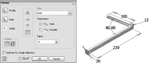
Finish the sketch, and select the Sweep command. If you have a single sweep profile, then it should automatically select the profile and pause for you to select a path.
Select a line in the path sketch to set it as the path.
Note that you can select either Solid or Surface for the feature. The sweep type will default to Path, and the orientation will default to Path also. The Sweep command also has an option to taper the sweep feature, as shown in Figure 5.3.
A number less than zero for the taper will diminish the cross section as the profile follows the path. A positive number will increase the cross section. If the taper increases the cross section at the radius of the path to a value that exceeds the radius value, then the feature will fail because this will create a self-intersecting path.
Adjust the taper to a negative value to see the preview update. Note that if you enter a positive value that's 0.5 or more, the preview will fail, indicating a self-intersecting path. Set the taper back to 0, and click OK to create the sweep.
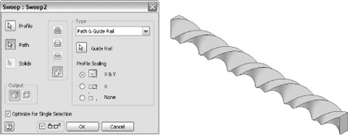
Although sweeping along a path is the default option, you can also utilize the Path & Guide Rail or Path & Guide Surface option to control the output of the Sweep command. These options provide additional control for more complex results. Often these options are utilized on sweeps based upon a 3D sketch path, but this is not required.
The Path & Guide Rail option provides a means to control the orientation of a profile as it is swept along a path. In Figure 5.4, the rectangular sweep profile will be swept along the straight path but controlled by the 3D helical rail. This approach is useful for creating twisted or helical parts.
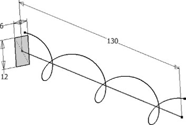
The 3D helical rail is guiding the rotation of the profile even though the sweep profile is fully constrained with horizontal and vertical constraints. Creating this part starts with creating the sweep path as the first sketch, followed by creating a second sketch perpendicular to the start point of the sweep path. The 3D helical rail is created using the Helical Curve command in a 3D sketch.
Open the file
mi_5a_004.iptfrom the Chapter 5 directory of the Mastering Inventor 2010 folder.Click the Sweep button on the Model tab.
Change the Type drop-down to Path & Guide Rail, choose the straight line as the path and the helix as the guide rail, and then click OK. Your result should resemble Figure 5.5.
At times you will need to sweep a profile that will conform to a specific shape and contour. This is often necessary when working with complex surfaces, particularly when cutting a path along such a surface. In the following exercise, you will use some surface tools to manipulate a solid shape while exploring the sweep guide's Surface option.
On the Get Started tab, click Open, and open the file named
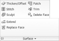
mi_5a_006.iptfound in the Chapter 5 folder.Click the small arrow on the Surface panel of the Model tab to see the Replace Face tool. Figure 5.6 shows the Surface panel expanded.
Click the Replace Face tool, select the red face as the existing face, then select the wavy surface for the new face, and finally click OK.
Right-click ExtrusionSrf1 in the browser, and select Visibility to turn it off.
Click the Plane button on the Model tab, click and hold down on the yellow surface, and then drag up to create an offset work plane at 85mm.
Right-click the edge of the work plane, and choose New Sketch.
Use the Project Geometry tool, and select the wavy face. This will result in a projected rectangle in your sketch.
Create a circle with the center point at the midpoint of the projected rectangle and tangent point on the corner of the rectangle so that your results look like the image on the left of Figure 5.7. Click the Finish Sketch button to exit the sketch.
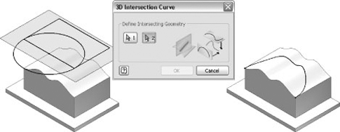
Click the Create 3D Sketch button on the Sketch panel.
Click the Intersection Curve tool from the 3D Sketch tab, and choose the circle and the wavy face. The result will be a curve as shown on the right of Figure 5.7. Turn the visibility of the 2D sketch and the work plane off.
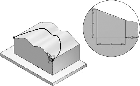
Create a 2D sketch on the front face, as shown in Figure 5.8. Be sure to select the projected edges and make them construction lines so that Inventor won't pick up the entire front face as a sweep profile. When the sketch is complete, click Finish Sketch.
Next select the Sweep tool, and choose the profile you just sketched for the profile input.
Select the 3D intersection curve for the path.
Click the Cut button to ensure that this sweep removes material from the part, and click OK.
The resulting cut sweep will be too shallow in some places, as shown on the left of Figure 5.9.
Edit the Sweep, and set the Type drop-down to Path & Guide Surface. Select the wavy surface as the guide surface, and then click OK. The result will look like the image on the right of Figure 5.9.
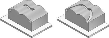
Whereas a sweep allows the creation of single profile extruded along a path, lofted features allow the creation of multiple cross-sectional profiles that are utilized to create a lofted shape. The Loft command requires two or more profile sections in order to function. Rails and control points are additional options to help control the shape of a lofted feature. A good example of lofted shape is a boat hull.
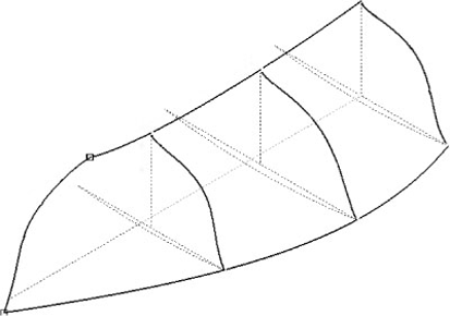
You could create a hull by defining just the section profiles, but you can gain more control over the end result by creating a loft with rails. Figure 5.10 shows the completed wireframe geometry to create a section of a boat hull. The geometry includes four section sketches, each composed of a 2D spline. There are two rails: the top and bottom composed of 3D sketch splines.
On the Get Started tab, click Open, and open the file named
mi_5a_008.iptfound in the Chapter 5 folder.Select the Loft tool in the Model browser.
Since the four section sketches are open profiles, the Loft command will automatically set the output to Surface. Select the four cross section sketches in consecutive order, front to back or back to front.
Then click Click To Add in the Rails section of the dialog box, and select 3D sketches named Rail1 and Rail2.
If you have the Preview option selected at the bottom of the dialog box, you should see a preview of the surface indicating the general shape, as shown in Figure 5.11. Click OK, and the surface will be created.
That concludes the lofting part of the boat hull, but if you'd like, you can continue with the following steps to learn a bit more about working with surfaces.
To finish the hull, select the Mirror tool on the Pattern panel of the Model tab.
Select the hull surface for the Features selection, and then click the Mirror Plane button.
Expand the Origin folder in the browser, click YZ to use as the mirror plane, and click OK.
Next you will create a 3D sketch to create a line for the top edge of the transom (back of the boat); right-click in the graphics window, and choose New 3D Sketch.
Click the Include Geometry button, and select the back edges of the hull.
On the 3D Sketch tab, click the Line tool, and draw a line across the back of the boat to form the top of the transom. Draw another line across the bottom of the transom where the two sides do not quite meet. Click Finish Sketch when the lines are drawn.
Select the Boundary Patch tool on the Surface panel, and select your 3D sketch lines and the projected geometry to create a surface for the transom. When creating boundaries, you need to select the line in the order that occurs in the boundary. Click Apply, and then create another boundary patch across the top by selecting the two edges of the side and the top edge of the transom.
You'll notice the gap in the base of the hull. Use the Boundary Patch tool to create a surface by clicking both edges of the gap and the small edge at the bottom of the transom.
Next, select the Stitch tool on the Surface panel, and select all five of the surfaces you created. It's easiest to window select them all at once.
Then click Apply and Done.
You should now have a solid boat. Of course, you would probably like to shell it out at this point. Before doing so, be sure to save your file. This is just good practice before running calculation-intensive operations like the shell tool, particularly on free-form shapes like this boat hull.
Once your file has been saved, select the Shell tool on the Modify panel of the Model tab.
Click the top face for the Remove Faces selection, and set Thickness to 10mm.
If your system is a bit undersized, you might want to skip the next two steps and just click OK now to let the shell solve for just one thickness. Otherwise, you'll specify a unique thickness for the transom.
Click the >> button to reveal the Unique Face Thickness settings, click the Click To Add row, and then click the transom face.
Set the unique face thickness value to 30mm, and click OK to build the shell.
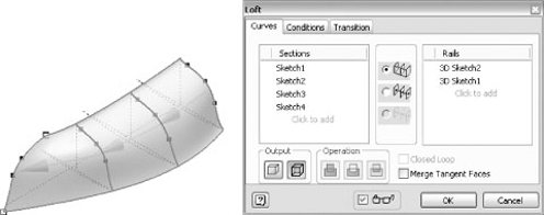
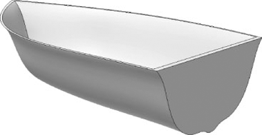
Figure 5.12 shows the completed boat. Of course, if you are a boat designer, you might see a few areas of the design that need improvement.
Area loft is used in the design of components where the flow of a gas or liquid must be precisely controlled. Area loft is a different way of controlling the finer points of creating a loft shape. Figure 5.13 illustrates what might be considered a fairly typical loft setup, consisting of three section profiles and centerline. The goal here is to create a loft from these profiles but to create a fourth profile to control the airflow through the resulting part cavity so that it can be choked down or opened up.
On the Get Started tab, click Open, and open the file named
mi_5a_010.iptfound in the Chapter 5 folder.Start the Loft tool, and select the three sections in order starting with the small rectangle.
Right-click, choose Select Center Line, and then click the centerline sketch line.
Right-click again, and choose Placed Sections; notice as you choose an option from the right-click menu that the dialog box updates to reflect your selections.
Slide your mouse pointer over the centerline, and then click roughly halfway between the circular section and the middle section.
Once you click a location, the Section Dimensions dialog box appears, as shown in Figure 5.14, giving you control over the position and section area of the placed section. You can switch the position input from Proportional where you enter a percentage of the centerline length to Absolute, which allows you to enter an actual distance if you know it.
In the Section Size area, you specify the actual area or set a scale factor based on the area of the loft as calculated from the sections before and after the one you are creating. On the far left, you can switch the section from driving to driven, letting the area be calculated from the position. Any number of placed sections can be used to create precise control of the feature.
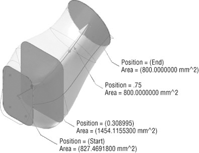
Leave Position set to Proportional Distance, change the position to .75, set the area to 800 (as shown in Figure 5.14), and click OK. You can access the section again by double-clicking the leader information.
Double-click the End section leader text, and change it from driven to driving using the radio buttons on the left. Notice that you can set the area but not the position.
Change the area to 800, and then click OK.
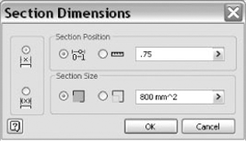
Figure 5.15 illustrates the placed loft section and the modified end section.
The centerline loft feature allows you to determine a centerline for your loft to follow, just like you did with the area loft. In the following steps, you'll create a centerline loft and look at some of the other options available in lofted features as well:
On the Get Started tab, click Open, and open the file called
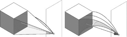
mi_5a_012.iptfound in the Chapter 5 folder.Click the Loft button, and select the red face of the solid block and the work point at the end of the arc as sections.
Right-click, choose Select Centerline, and then click the arc. Notice how the lofted shape now holds the centerline, as shown in Figure 5.16.
Click the Conditions tab in the Loft dialog box so that you can control the curve weight and transition type at the work point and square profile.
Click the drop-down next to the Edges section, and set it to Tangent. Change the weight to 2 so the curve extends out from the box.
Set the Work Point drop-down to Tangent also, and set the weight to 6.
Currently, the loft is extending out past the work plane. Often this can be a problem because the work plane may have been established at the overall length of the part. To resolve this, set the drop-down to Tangent To Work Plane, and select the work plane on the screen. Notice the adjustment. Figure 5.17 shows the preview of the adjustments.
Use the Split tool to trim the end of the lofted shape. Right-click the work plane named Trim Plane in the browser, and choose Visibility.
Select the Split tool on the Modify panel of the Model tab.
Set the method to Trim Solid (middle button on the left), and select the trim plane as the Split tool.
Change the Remove direction so that the tip of the loft is the part being removed, and click OK. Figure 5.18 shows the loft with the tip trimmed.
Here is the full list of conditions, depending upon the geometry type:
- Free Condition
No boundary conditions exist for the object.
- Tangent Condition
This condition is available when the section or rail is selected and is adjacent to a lateral surface, body, or face loop.
- Smooth (G2) Condition
This option is available when the section or rail is adjacent to a lateral surface or body or when a face loop is selected. G2 continuity allows for curve continuity with an adjacent previously created surface.
- Direction Condition
This option is available only when the curve is a 2D sketch. The angle direction is relative to the selected section plane.
- Sharp Point
This option is available when the beginning or end section is a work point.
- Tangent
This option is available when the beginning or end section is a work point. Tendency is applied to create a rounded or dome-shaped end on the loft.
- Tangent To Plane
This is available on a point object, allowing the transition to a rounded dome shape. The planar face must be selected. This option is not available on centerline lofts.
The angle and weight options on the Conditions tab allow for changes to the angle of lofting and the weight value for an end condition transition. In this example, if the endpoint condition is changed to Tangent on the work point, the weight is automatically set to 1 and can be adjusted. Click the weight, and change it to 3 to see how the end condition will change in the preview. Experiment with the weight to see the changed conditions. If a value is grayed out, then the condition at that point will not allow a change.
There are a couple of things to keep in mind when creating sketches to be used as lofts. First, you should always project the endpoints of rails into your profile sketches, or vice versa, so that the rail will map to the profile correctly. Second, it often helpful to create work surfaces or helper geometry to sketch on so that you know you are working in the right location and orientation as you sketch. In these steps, you'll create a lofted surface and use it to create a lofted solid:
On the Get Started tab, click Open, and open the file named
mi_5a_014.iptfound in the Chapter 5 folder.Extrude the rectangle up 30mm, making sure to do so as a surface rather than a solid (select the surface output in the Extrude dialog box).
Create a sketch on each side of the extruded surface, and then create the sketches on the ends. Both side sketches are the same sketch but will be located opposite one another. The same is true of the ends. Be sure that you project the referenced edges and set all projected geometry as construction lines. Figure 5.19 shows the sketches; note the projected points on the end sketch.
Use the Loft tool, and choose the two end sketches as the sections and the two side sketches as rails; the result will be a twisted surface (if you forgot to make the projected geometry construction lines, you will need to set the output to surface in the Loft dialog box in order to select just the arcs).
Use the Mirror tool, and mirror the lofted surface to both sides of the XY origin plane.
On the Surface panel, select the Extend Surface tool (use the drop-down arrow on the Surface panel to reveal this tool).
Ensure that the Edge Chain option is selected, and then select all the edges of the rectangular surface.
Set the Extents drop-down to the To option, and then select the mirrored surface. Then click OK.
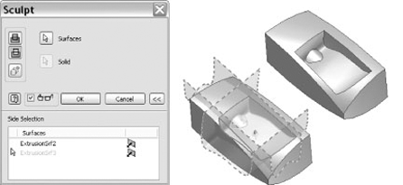
Select the Sculpt tool on the Surfaces panel, select all three of the surfaces, and then click OK to create the solid. Figure 5.20 shows the results of the Sculpt tool.
The Sculpt tool can use surfaces, work planes, and solid faces as 3D boundaries to "flood fill" any volume that exists. If there is not a "water-tight" volume, no solid can be created. You can use Sculpt to cut material from a solid as well. When cutting with Sculpt, the profile can be open. This tool differs from the Stitch tool in that surfaces do not need to be trimmed and in its ability to cut material. Figure 5.21 shows the result of uses the Sculpt tool to cut the combined volume of two open profile extruded surfaces from a solid. Notice that the >> button as been expanded to reveal the direction controls, allowing the user to choose which side of the surface to sculpt/cut.
It is possible to create a multi-body part file with separate solids representing each part of an assembly and then save the solids as individual parts, even having them automatically placed into an assembly. Creating multiple solid bodies in a single part file offers some unique advantages compared to the traditional methods of creating parts in the context of an assembly file. For starters, you have one file location where all your design data is located. Second, it is often easier to fit parts together using this method, by simply sketching one part right on top of the other, and so on.
These two advantages are also the main two disadvantages. Placing large amounts of data (and time and effort) into a single file can be risky should that file be lost. And creating a part with an overabundance of interrelated sketches, features, and solid bodies can create a "house of cards" situation that makes changing an early sketch, feature, or solid a risky endeavor. Used wisely, though, multi-body parts are a powerful way to create tooling sets, molds, dies, and other interrelated parts.
If you do large machine design, you would be best off to create many smaller multi-body part files rather than attempting to build one large one. Or you might find that using multi-body parts will work well for certain interrelated components, while using traditional part/assembly techniques works for the rest of the design.
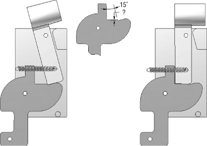
In the following steps, you'll explore the creation of multi-body parts by building a simple trigger mechanism. The challenge here is to define the pawl feature on the trigger lever as it relates to the hammer bar. Figure 5.22 shows the trigger mechanism in its set position on the left and at rest on the right. As the trigger lever is engaged, the hammer bar overcomes the pawl (lip), and the spring is allowed to force the hammer bar to swing.
On the Get Started tab, click Open, and open the part named
mi_5a_016.iptfound in the Chapter 5 folder.Create a sketch on the red face of the plate.
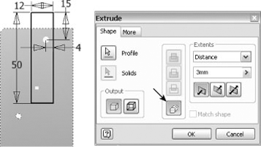
Create a rectangle, as shown in Figure 5.23.
Extrude the rectangle 3mm away from the plate, and use the New Solid option in the Extrude dialog box (leave the circle unselected from your extrude profile so that you end up with a hole).
When you click OK, you'll see that the Solid Bodies folder in the model tree now shows two bodies present, the plate and the hammer bar.
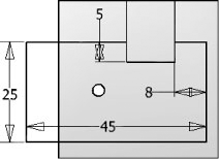
Create another sketch on the front of the plate, and create another rectangle toward the bottom, referencing the end of the hammer bar as shown in Figure 5.24.
Extrude the rectangle 3mm away from the plate, use the New Solid option in the Extrude dialog box, and then click OK. This completes the base feature for the trigger lever.
Expand the Solid Bodies folder in the browser, and notice there are three solids listed (if you see less than three, edit your extrusions, and make sure you used the New Solid option).
Double-click the solid that is your hammer bar, and rename it Hammer Bar, for reference later. Here are several things to note at this point:
If you expand the browser node for each one, you can see the features involved in each.
You can right-click a solid or solids, choose Hide Others to isolate just the selected ones, and then use Show All to bring back any hidden solids.
You can select the solid and then choose a color style from the Color Override drop-down on the Quick Access toolbar (at the very top of your screen).
You can right-click each solid and choose Properties to set the name and color, view the pass properties, and strip previous overridden values.
Next you'll create the notch in the trigger lever. To do so, however, you will first make a copy of the hammer bar and then turn that solid into a solid that represents the hammer bar in both the set and not set positions. After that, you'll cut that solid away from the trigger lever.
Select the Copy Object tool on the Modify panel, and then click the hammer bar for the selection. Leave all the other setting as is, and click OK.
Next select the Sculpt tool on the Surface panel, and choose the composite surface you just created with the Copy Object tool.
Set the output to New Solid, and click OK.
Expand the Solid Bodies folder, right-click the solid you just created (it is most likely named Solid4), and choose Hide Others.
Rotate the view slightly, and then choose the Circular Pattern tool on the Patterns panel.
Select the solid on-screen for the Features selection, click the edge or face of the hole for the rotation axis, and set the placement count and angle to 2 and 15 degrees, respectively.
Ensure that the rotation direction is going counterclockwise, use the flip button if not, and then click OK. The resulting solid will be a combination of the hammer bar in its original and rotated positions.
Right-click the solid in the browser and choose Show All to bring the other objects back on-screen.
Select the Combine tool on the Modify panel, and select the trigger lever for the Base selection.
Select the fused, rotated body for the tool body selection, and then set the operation type to Cut so that you are subtracting from the trigger lever. Then click OK.
Now that you've solved the trigger pawl shape and size by using a multi-body part, you can finish the parts by adding features to each body. You'll note that if you create an extrusion, for instance, you can select which solid to add that extrusion to. If it is a cut extrusion, you can select multiple bodies and cut them all at once. The same is true of fillets, holes, and so on.
You can also use the Move Bodies tool to reposition solids, once they are created. Try it on your trigger mechanism parts. Note that you have to click the edges or outlines of the preview object, rather than on a face or on the original object as you might suppose. Figure 5.25 shows the Move Bodies options.
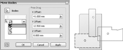
- Free Drag
Move via X, Y, or Z offsets, or better yet, just click it and drag it.
- Move Along Ray
Select an edge or axis to define the move direction, and then specify an offset value or just click and drag it in that direction.
- Rotate
Select an edge or axis to define the rotational pivot, and then specify an angle or click and drag it.
- Click to Add
Create as many move actions as you want and do them all at once.
Another tool that you may find useful when working with multi-body parts is the Split tool. For instance, if you create a part and then model the mold form about it, you can use a work plane or user-created surface to split the form along a parting line.
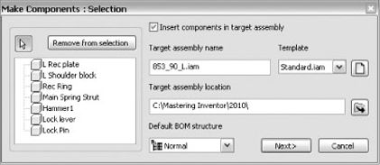
Once you have created your multi-body part, you can write out each solid as an individual part file. The resulting part files are what are known as derived parts. You can think of these derived parts as just linked copies of the solid bodies. If you make a change in the multi-body part, it will update the derived part. You can break the link or suppress the link in the derived part as well.
Additionally, you can choose to take your multi-body part and write the whole thing to an assembly. The assembly will consist of all the derived parts placed just as they exist in the multi-body part. These files will be grounded in place automatically so that no assembly constraints are required to hold them in place. If you decide you would like to apply constraints to all or some of the parts, you can unground them and do so, as well as organize them into subassemblies, and so on.
You should be aware too that any additional modeling that you do in the derived part or assembly will not push back to the multi-body part file. Although this may seem like a limitation, it can also be viewed as a good thing, allowing for the separation of design tasks that some design departments require. Here are the general steps for creating components from a multi-body part file:
Click the Make Components button on the Manage tab, and then select the solid bodies you want to create parts of.
Select additional solids to add to the list or select from the list, and click Remove From Selection to exclude any solids that you decide you do not want to create parts from.
Select Insert Components In Target Assembly, and then set the assembly name, the template from which to create it, and the save path, or clear this option to create the parts only. If the assembly already exits, use the Target Assembly Location's Browse button to select it.
Click Next to accept your selections, as shown in Figure 5.26.
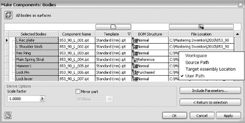
The next dialog box allows you to name and set paths for the derived parts. Click the cells in the table to make changes for the parts as required:
Click or right-click the cells to choose from the options for that cell type, if any.
You can shift select multiple components and use the buttons above the Template and File Location columns to set those values for multiple parts at once.
Click Include Parameters to choose which layout model parameters to have present in the derived parts.
Click Apply or OK to make the components, as shown in Figure 5.27. If the component files are created in an assembly, the assembly file is created with the parts placed and left open in Inventor, but the assembly and parts are not saved until you choose to do so. If you choose to create the parts without an assembly, you are prompted to save the new files.
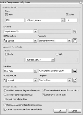
You can set default behaviors of the Make Components dialog box in a multi-body part file (or a template file) by going to the Tools tab, clicking Document Settings, going to the Modeling tab in the dialog box that opens, and clicking the Options button. Figure 5.28 shows these options.
You can create parts derived from other components using the Derive tool. Common uses of the Derive tool are to create scaled and mirrored versions of existing parts, to cut one part from another part, and to consolidate an assembly into a single part file. Nonlinear scaling is accomplished using an add-in available in the Inventor installation directory.
Derived parts are base solids that are linked to the original feature-based part. Modifications are allowed to the derived part in the form of additional features. Original features are modified in the parent part, and changes in modification to the parent part are moved to the derived part upon save and update. There is no reasonable limit to the number of times the parent part or succeeding derived parts can be again derived into more variations.
To derive a single part file, follow these steps:
From a new part file, select the Manage tab, and then click the Derive tab.
In the Open dialog box, browse to the part file, and then click the Open button.
Select from one of these derived styles:
A single solid body with no seams between faces that exist in the same plane
A single solid body with seams
One or more solid bodies (if the source part contains multiple bodies)
A single surface body
Use the status buttons at the top to change the status of all the selected objects at once, or click the status icon next to each individual object to set the include/exclude status.
Optionally, click the Select From Base button to open the base component in a window to select the components.
Specify scale factor and mirror plane if desired.
Click OK.
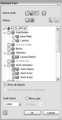
If the part being derived contains just one body, it is displayed on-screen. If the part being derived is a multi-body part with only a single body set as visible in the part, it is displayed on-screen. If the part being derived is a multi-body part with more than one visible body, none of the bodies is displayed on-screen. Select the bodies to include by expanding the Solid Bodies folder and toggling the status. To include all bodies, select the Solid Bodies folder, and then click the Include Status button. Figure 5.29 shows the Derived Part dialog box.
To derive an assembly file, follow these steps:
From a new part file, select the Manage tab, and then click the Derive tab.
In the Open dialog box, browse to the assembly file, and then click the Open button.
Select from one of these derived styles:
Use the status buttons at the top to change the status of all the selected objects at once, or click the status icon next to each individual object to set the include/exclude status.
Optionally, click the Select From Base button to open the base component in a window to select the components.
Click the Other tab to select which component sketches, work features, parameters, iMates, and part surfaces to include in the derived assembly.
Click the Representations tab to use a design view, positional, and/or level of detail representation as the base for your derived part.
Click the Options tab to remove geometry, remove parts, fill holes, scale, and/or mirror the assembly.
Click OK. Figure 5.30 shows the Derived Assembly dialog box.
Often you will need to modify a derived part source file after having derived it into new part. In order to do so, you can access the source part or assembly from the Model browser of the derived part by double-clicking it in the browser or by right-clicking it in the browser and choosing Open Base Component. The original file is opened in a new window where you can make changes as needed. To update the derived part to reflect changes to the source file, use the Update button found on the Quick Access toolbar (top of the screen).

You can edit a derived part or assembly by right-clicking it in the browser and choosing Edit Derived Part or Edit Derived Assembly. This will open the same dialog box used to create the derived part so that you can change the options and selections you set when the derived part was created. Updates will be reflected in the file when you click OK. The Edit Derived Part or Edit Derived Assembly options are unavailable if the derived part needs to be updated.
You can also break or suppress the link with the source file by right-clicking the derived component in the browser and choosing the appropriate option. Updates made to the source file will not be made to the derived part when the link is suppressed or broken. Suppressed links can be unsuppressed by right-clicking and choosing Unsuppressed Link From Base Component. Breaking the link is permanent and it cannot be restored.
Another way to derive components is to use the Derive Component tool on the Assembly Tools tab while in an assembly file. This tool allows you to select a part on-screen (or select a subassembly from the browser) and then specify a name for the new derived part file. You'll then be taken into the new derived part file. The resulting derived part or assembly uses the default derive options and the active assembly representations as they are saved in the source file. You can use the edit option in the derived part to change the settings if needed.
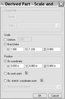
You can accomplish nonlinear part scaling in Autodesk Inventor by using an add-in that you can find at C:Program FilesAutodeskInventor 2010SDK. The first time you access the SDK folder, you will need to unpack the user tools by double-clicking the UserTools.msi file.
Once the tools are unpacked, you can go to C:Program FilesAutodeskInventor 2010SDKUserToolsDerivedPart_SP and run the Install.bat file. After installing the macro, a Derived Part (Scale/Position) button will be available on the Add-Ins tab. Selecting the Derived Part (Scale/Position) button will introduce a new dialog box, shown in Figure 5.31, permitting you to browse to the part file that will be scaled and allowing individual X, Y, and Z scale value inputs. You can use the same button to edit the derived component or right-click as you would any other derived component. Please note that this is not part of the Inventor software that is officially supported by Autodesk and is provided for your use as is.
Inventor includes two tools to create patterns:
The Circular Pattern tool does just what you'd expect it to; it patterns a feature or set of features around an axis. The Rectangular Pattern tool also does what you'd expect, plus more. Using the Rectangular Pattern tool, you can create a pattern along any curve. If you select two perpendicular straight lines, edges, or axes, the result will be a rectangular pattern. However, if you select an entity that is not straight, the pattern will follow the curvature of the selected entity also.
Rectangular patterns use straight edges to establish the pattern directions. You can select a single feature or several features for use in the pattern. Be sure to check the Model browser to see that you have only the features that you intend to pattern select, because it is easy to accidentally select base features when attempting select negative cut features. Start your exploration of patterns by creating a simple rectangular pattern, as shown here:
On the Get Started tab, click Open.
Browse for the file named
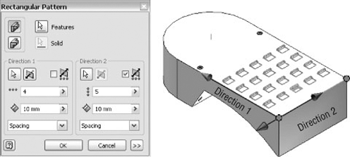
mi_5a_018.iptlocated in the Chapter 5 directory of the Mastering Inventor 2010 folder, and click Open.Select the Rectangular Pattern tool on the Pattern panel of the Model tab.
With the Features button enabled, select the three features whose names start with the word switch in the browser.
Right-click, choose Continue to set the selection focus from Features to Direction1, and then click the straight edge, as shown in Figure 5.32. Use the Flip Direction button to ensure that direction arrow is pointing toward the round end of the part.
Set the count to 4 and the spacing length to 10mm
Click the red arrow button under Direction2 to set it active, and then click the straight edge along the bottom, as shown in Figure 5.32.
Set the count to 5 and the spacing length to 10mm
Click the Midplane check box in the Direction2 settings to ensure that you get two instances of the pattern to each side of the original.
Click OK.
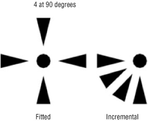
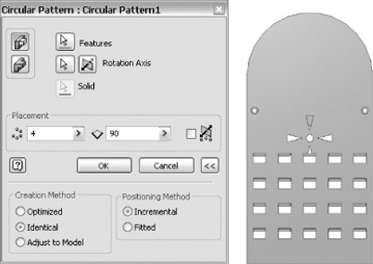
You can pattern features around an axis using the Circular Pattern tool. Angular spacing between patterned features can be set in two ways:
- Incremental
Positioning specifies the angular spacing between occurrences.
- Fitted
Positioning specifies the total area the pattern occupies.
Figure 5.33 shows the same pattern of four occurrences at 90 degrees but set with different positioning methods.
You can enter a negative value to create a pattern in the opposite direction, and you can use the Midplane check box to pattern in both directions from the original. Continue from the previous exercise with the open file, or open mi_5a_020.ipt to start where that exercise ended:
In the Model browser, select the end-of-part marker, and drag it down below the feature named Indicator Cut.
Select the Circular Pattern tool on the Pattern panel of the Model tab.
With the Features button enabled, select the feature named Indicator Cut.
Right-click and choose Continue to set the selection focus from features to axis.
Select the center face of the feature named Indicator Stud Hole.
Set the count to 4 and the angle to 90; then click the >> button.
In the Positioning Method area, click the Incremental option so that the four occurrences of the pattern are set 90 degrees apart, rather than being fit into a 90-degree span. Alternatively, you could set the angle to 360 and leave the positioning method to Fitted and get the same result.
Click OK. Figure 5.34 shows the circular pattern.
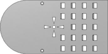
You'll note that your patterned objects require some adjustments. One of the occurrences interferes with the switch feature, and the other does not cut through the part correctly. To resolve this, you will first edit the circular pattern and change the way the occurrences solve, and then you'll suppress the occurrence of the switch feature in the rectangular pattern.
Right-click the circular pattern in the browser and choose Edit Pattern, or double-click it in the browser.
Click the >> button to reveal the Creation Method area, and then select the Adjust To Model option. This allows each instance of the pattern to solve uniquely based on the geometry of the model when the feature is using a Through or Through All termination solution.
Expand the Rectangular Pattern in the browser to reveal the listing of each pattern occurrence.
Roll your mouse pointer over each occurrence node in the browser until you see the one that interferes with the circular pattern highlight.
Right-click that occurrence, and choose Suppress.
Any occurrence other than the first can be suppressed to allow for pattern exceptions or to create unequal pattern spacing. Figure 5.35 shows the adjusted patterns.
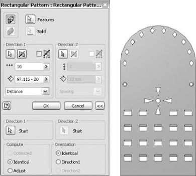
Although the Circular Pattern tool allows you to pattern objects around a center axis, it does not provide a way to keep the patterned objects in the same orientation as the original. To do so, you can use the rectangular pattern. Keep in mind that the term rectangular pattern is a bit of a misnomer; this tool might more accurately be described as a curve pattern tool, because it allows you to select any curve, straight or not, and use it to determine the pattern direction(s). Continue from the previous exercise with the open file, or open mi_5a_022.ipt to start where that exercise ended:
In the Model browser, select the end-of-part marker, and drag it down below the feature named Pin Insert Path Sketch.
Select the Rectangular Pattern tool on the Pattern panel of the Model tab.
With the Features button enabled, select the feature named Pin Insert Cut.
Right-click and choose Continue to set the selection focus from features to Direction1.
Click the sketched curve (line or arc).
Set the count to 10, and notice that the preview extends out into space.
Click the >> button to reveal more options.
Click the Start button in the Direction1 area, and then click the center of the Pin Insert Cut on-screen to set that center point as the start point of the pattern.
Change the solution drop-down from Spacing to Curve Length, and note that the length of the sketch curve is reported in the length box.
Change the solution drop-down from Curve Length to Distance, and then type −14 at the end of the length value to compensate for the start and end point adjustments.
Toggle the Orientation option from Identical to Direction1 to see the difference in the two, and then set it back to Identical.
Click OK. Figure 5.36 shows the resulting pattern.
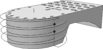
In addition to creating patterns based on edges and sketches, you can use surfaces to define the pattern direction. In this exercise, you'll create a surface coil to use as a pattern direction. You can continue on from the previous exercise with the open file, or you can open mi_5a_024.ipt to start where that exercise ended.
In the Model browser, select the end-of-part marker, and drag it down below the feature named Coil Pattern Sketch.
Select the Coil tool on the Model tab.
Next choose the line segment in the Coil Pattern Sketch at the base of the part for the profile.
Select the visible work axis in the center of the part for the axis.
Click the Coil Size tab, and set the type to Revolution and Height.
Click OK.
You'll now create two work points based on the coil location for use in placing holes. Once the holes are placed, you can pattern them using the surface coil.
Click the Point button on the Work Features panel of the Model tab, and select the vertical tangent edge and the surface coil to create work points at the intersections, as shown in Figure 5.37.
Click the Hole tool on the Model tab, and set the Placement drop-down to On Point.
Select one of the work points for the Point selection, and then select the flat side face of the part to establish the direction.
Set the termination drop-down to To, and then select the inside circular face of the part. Then click Apply.
Repeat the previous two steps to place the second hole, and then click OK.
Click the Rectangular Pattern button on the Model tab.
Click the two holes for the features, and then right-click and choose Continue.
Select the surface coil for Direction1.
Set the count to 10 and the length to 10mm.
Click the >> button, and choose Direction1 for the orientation.
Set the Compute option to Adjust, and then click OK.
Right-click the coil and work points and turn off the visibility of these features. Figure 5.38 shows the pattern.
Oftentimes a part can be modeled as a base feature and then patterned as a whole in order to create the completed part. Once patterned, nonsymmetric features can be added, and/or patterned occurrences can be suppressed. You can also use the Pattern Entire Solid option to create separate solid bodies when creating multi-body part files is the goal. To take a look at patterning these options, open the part named open mi_5a_028.ipt, and follow these steps:
Select the Rectangular Pattern tool on the Pattern panel of the Model tab.
Click the Pattern A Solid button so that the entire part is selected to be patterned. Notice the two buttons that appear in the top-right corner of the dialog box:
- Join
This option is used to pattern the solid as a single solid body.
- Create New Bodies
This option is used to the solid as separate solid bodies, for multibody part creation. Leave this option set to Join.
Set Direction1 to pattern the solid in the direction of the part four times at a spacing of 10mm.
Set Direction2 to pattern the solid in the direction of the part thickness two times at a spacing of 3mm, as shown in Figure 5.39.
Next, expand the pattern in the Model browser, and right-click to suppress the two middle occurrences on the top level. Roll your mouse pointer over each occurrence to see it highlight on-screen to identify which occurrences are the correct ones. Figure 5.40 shows the results of suppressing the correct occurrences.
Now you'll pattern the entire solid again, select the Rectangular Pattern tool again, and click the Pattern A Solid button.
Set Direction1 to pattern the solid in the direction of the part length two times at a spacing of 50mm.
Set Direction2 to pattern the solid in the direction of the part width two times at a spacing of 40mm, as shown in Figure 5.41.
Create a new 2D sketch on one of the long narrow faces, and project the tangent edge of the slot cuts, or sketch a rectangle on the face. Do this for both ends of the face. Then use the Extrude tool, set the extents to To, and select the vertex as shown in Figure 5.42. The result will be the removal of all the partial slot features.
Create another sketch on the same face and sketch an arc from corner to corner, and set the radius to 400mm. Then use the Extrude tool to extrude just the arc as a surface (click the Surface Output button in the Extrude dialog box). Set the extents to To again, and select the same vertex as you did before.
Select the Replace Face tool from the Surface panel of the Model tab. You may have to expand the arrow on the Surface panel to expand the drop-down in order to find the Replace Face tool.
Select the two recessed faces for the existing faces selection, and then select the extruded surface for the new faces selection, as shown in Figure 5.43.
Next create a sketch on the top face, and create two rectangular profiles to use for creating an extrude cut, as shown in Figure 5.44. This cut removes the middle slots and holes resulting in two long slots down the middle.
Finally, select the Shell tool from the Modify panel. Choose the bottom face as the Remove Faces selection, and set the Thickness to 1mm. Figure 5.45 shows the finished part from the top and bottom views.

It is often desirable to have standard hole spacing set up to dynamically update based on changes to the overall length. You can do this by setting up your patterns with formulas to calculate the spacing from the length parameter. Parts set up in this way can then be saved as template parts, allowing you to select them for new part creation and simply edit the length parameter. To set up a dynamic pattern, open the file named mi_5a_032.ipt, and follow these steps:
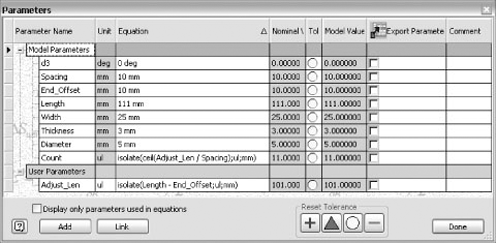
Click the Manage tab, and select the Parameters tool.
Notice that many of the dimensions in this part have been named. This is good practice when creating formulas. To create a formula to determine the spacing, click the Add button in the lower-left corner of the dialog box. This will create a new user-defined parameter. Enter Adjust_Len for the parameter name (recall that you are not allowed spaces in parameter names).
Click the unit cell, and set the Units to ul, meaning unitless.
Type isolate(Length - End_Offset;ul;mm) into Equation column. There are two parts to this equation:
- Length – End_Offset
Subtracts the distance from the end of the part from the overall length of the part
- Isolate(expression; unit; unit)
Neutralizes the distance unit mm so that the Adjust_Len parameter can read it as unitless
Next click the cell for Count equation, and enter isolate(ceil(Adjust_Len / Spacing);ul;mm) into the cell. There are three parts to this equation:
- Adjust_Len/Spacing
Divides the adjusted length distance by the value specified in the pattern spacing
- Ceil(expression)
Bumps the value up to the next highest whole number
- Isolate(expression; unit; unit)
Neutralizes the distance unit mm so that the Count parameter can read it as unitless
Next, click the Done button, and then use the Update button to update the part (you can find the Update button on the Quick Access bar at the top of the screen). Figure 5.46 shows the parameter dialog box.
You may notice that because the length value is currently set to 111mm that the last hole is running off the part. Because the equation used the Ceil function to bump the calculated value to the next whole number, the count will always be on the high end. Depending upon the part length, this may leave you with an extra hole. You can suppress the occurrence of this hole in the Model browser quite easily. Another approach is to remove the Ceil function and allow Inventor to round the calculated value up or down automatically. Depending upon the length and spacing values, this might leave you with a missing hole at the end of the pattern, where a value gets rounded down. Both are valid options, and you can decide which works best for your situation.
Edit Extrusion1 to adjust the part length, and try different values to see how the count drops out. You can also open the files named mi_5a_033.ipt and mi_5a_034.ipt to examine similar hole patterns. In mi_5a_033.ipt, the pattern uses the Distance option in the pattern feature to evaluate the length of the part. It holds an end offset value and then spaces the holes evenly along that distance.
In mi_5a_034.ipt, the pattern is calculated from the center of the part rather than coming off one end. These are just a few examples of how to use user parameters to create dynamic patterns. There are other variations as well. In the next section, you'll take a more in-depth look at parameters.
Parameters in part and assembly files can provide powerful control over individual parts and assemblies while also improving efficiency within designs. Part parameters enable the use of iParts, which are a form of table-driven part. Assembly parameters enable the use of table-driven assemblies and configurations. Parameters are accessed through the Tools menu and within the Part Features and Assembly tool panels.
iProperties, generically known as Windows file properties, allow the input of information specific to the active file. The iProperties dialog box is accessed through the File drop-down in Inventor. The dialog box contains several tabs for input of information:
- The General tab
Contains information on the file type, size, and location. The creation date, last modified date, and last accessed date are preserved on this tab.
- The Summary tab
Includes part information such as title, subject, author, manager, and company. Included on this tab are fields for information that will allow searching for similar files within Windows.
- The Project tab
Stores file-specific information that, along with information from the Summary, Status, Custom, and Physical tabs, can be exported to other files and used in link information within the 2D drawing file.
- The Status tab
Allows the input of information as well as the design state and dates of each design step.
- The Custom tab
Allows the creation of custom parameters for use within the design. Parameters exported from the Parameters dialog box will also appear in the list. Formulas can be used within a custom parameter to populate values in preexisting fields within the Project and Status tabs.
- The Save tab
- The Physical tab
Allows for the changing of material type used in the current file and displays the calculated physical properties of the current part such as mass and moment of inertia, as determined by the material type.
Active use of iProperties will help the designer in improving overall productivity as well as the ability to link part and assembly information into 2D drawings. Adding search properties in the Summary tab will assist the user in locating similar files.
Part parameters are composed of model parameters, user parameters, reference parameters, and custom parameters. Model parameters are automatically embedded as a part is dimensioned and features are created. Most are a mirror image of the sketch creation process. As each dimension is created on a sketch, a corresponding model parameter is created, starting with a parameter called d0 and continuing with the label value being incremented each time a new parameter is created. When you name a dimension, you are changing the automatically assigned parameter name. To access the list of parameters, click the Manage tab, and select the Parameters button. Figure 5.47 represents a typical parameter list.
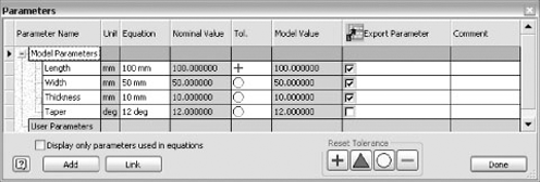
Looking at the columns across the top of the dialog box, you will see columns for the parameter name, unit type, equation, nominal value, tolerance type, model value, parameter export, and descriptive comments. Take a look at each of these columns:
- Model Parameters
The values in this column correspond to the name of the parameters assigned as the part is built. Each parameter starts with a lowercase d followed by a numeric value. Each of these parameters can be renamed to something that is more familiar such as Length, Height, Base_Dia, or any other descriptive single word. Spaces are not allowed in the parameter name. Hovering your mouse pointer over a name will initiate a tool tip that will tell you where that variable is used or consumed.
- Unit
The unit type defines the unit used in the calculation. Normally, the unit type will be set by the process that created it. When a user parameter is created, you will be presented with a Unit Type dialog box when clicking in the Unit column. This will allow you to select a particular unit type for the user parameter.
- Equation
This either specifies a static value or allows you to create algebraic style equations using other variables or constants to modify numeric values.
- Nominal Value
This column displays the result of the equation.
- Tolerance
This column shows the current evaluated size setting for the parameter. Click the cell to select Upper, Lower, or Nominal tolerance values. This will change the size of tolerance features in the model.
- Model Value
This column shows the actual calculated value of the parameter.
- Export Parameters
These check boxes are activated to add the specific parameter to the custom properties for the model. Downstream, custom properties can be added to parts lists and bills of materials by adding columns. Clearing the check box will remove that parameter from custom properties. After a parameter is added, other files will be able to link to or derive the exported parameter.
- Comment
This column is a descriptive column used to help describe the use of that parameter. Linked parameters will include the description within the link.
User parameters are simply user-created parameters. They are parameters that are created by clicking the Add button in the lower-left portion of the Parameters dialog box. User parameters can be used to store equations that drive features and dimensions in the model. The user-created parameter can utilize algebraic operators written in the proper syntax that will create an expression in a numerical value.
Reference parameters are driven parameters that are created through the use of reference dimensions in sketches and the use of derived parts, attached via a linked spreadsheet, created by table-driven iFeatures or created through the use of the application programming interface (API). For instance, Inventor sheet-metal parts create flat pattern extents, which are stored as reference parameters.
Custom parameters are either created manually in the custom tab of iProperties or created automatically by exporting individual parameters from the list. Custom parameters may be linked to drawings and assemblies for additional functionality.
The functions in Table 5.1 can be used in user parameters or placed directly into edit boxes when creating dimensions and features.
Table 5.1. Functions and Their Syntax for Edit Boxes
Unit Type | Description | |
|---|---|---|
| Unitless | Calculates the cosine of an angle. |
| Unitless | Calculates the sine of an angle. |
| Unitless | Calculates the tangent of an angle. |
| Angularity | Calculates the inverse cosine of a value. |
| Angularity | Calculates the inverse sine of a value. |
| Angularity | Calculates the inverse tangent of a value. |
| Unitless | Calculates the hyperbolic cosine of an angle. |
| Unitless | Calculates the hyperbolic sine of an angle. |
| Unitless | Calculates the hyperbolic cosine of an angle. |
| Angularity | Calculates the inverse hyperbolic cosine of a value. |
| Angularity | Calculates the inverse hyperbolic sine of a value. |
| Angularity | Calculates the inverse hyperbolic tangent of a value. |
| Unit^0.5 | Calculates the square root of a value. The units within the For example, |
| Unitless | Returns 0 for a negative value, 1 if positive. |
| Unitless | Returns an exponential power of a value. For example, |
| Unitless | Returns the next lowest whole number. For example, |
| Unitless | Returns the next highest whole number. For example, |
| Unitless | Returns the closest whole number. For example, |
| Any | Returns the absolute value of an expression. For example, |
| Any | Returns the larger of two expressions. For example, |
Any | Returns the smaller of two expressions. For example, | |
| Unitless | Returns the natural logarithm of an expression. |
| Unitless | Returns the logarithm of an expression. |
| Unit^expr2 | Raises the expression1 to the power of For example, |
| Unitless | Returns a random number. |
| Any | Used to convert the units of an expression. For example, |
| Internal Parameter | Returns the constant equal to a circle's circumference divided by its diameter 3.14159265359 (depending upon precision). For example, |
| Internal Parameter | Returns base of the natural logarithm 2.718281828459 (depending upon precision). |
| Any | Used to convert unit types of an expression much like isolate. For example,
|
Assembly parameters function in much the same way as part parameters, except that generally they will control constraint values such as offset and angle. When authoring an iAssembly, other parameters will be exposed for usage such as assembly features, work features, iMates, and component patterns, as well as other parameters that may exist within an assembly.
Autodesk Inventor allows you to analyze parts in a manner that ensures valid fit and function at dimensional extremes. When the parts are assembled within an Inventor assembly file, you can check to ensure that the parts can be assembled without interference. By specifying dimensional tolerances within parts, you are capturing valuable design data that will assist in manufacturing and assembly.
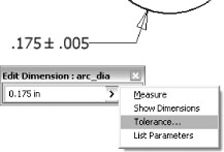
You can add tolerances to any individual sketch dimension by right-clicking and setting individual precision and tolerance values. Altering the dimension to adjust for tolerance and procession will not affect any other dimension within the part. Alternatively, global tolerancing can be specified within a part and will affect every dimension within the model.
Depending upon the particular design, allowable tolerances will be specified to ensure that the entire assembly will be within acceptable tolerances after manufacture and assembly. Inventor templates can be created, storing tolerance types and other settings for each standard. When the part is created using such a template, standard tolerance values can be overridden for specific dimensional values. If needed, you can override all tolerances within a file or just a specific dimension.
When considering part designs for manufacturing, be careful not to apply precise tolerance values where they are not necessary for the design and assembly. Excessive and unneeded tolerancing during the design phase can substantially increase the cost to manufacture each part. The secret to good design is to know where to place tolerances and where to allow shop tolerances to occur.
In the Parameters dialog box, you can set a parameter value to include the tolerance. The four options are as follows:
- Upper
The upper tolerance value in a stacked display. This value should Maximum Material Condition (MMC). For a hole, the smallest diameter is MMC, while for a shaft the largest diameter is MMC.
- Median
The midway point between the upper and lower tolerances. This is commonly used when CNC machines are programmed from the solid model.
- Lower
The lower tolerance in a stacked display. This value should be Least Material Condition (LMC). For a hole, the largest diameter is LMC, while for a shaft the smallest diameter is LMC.
- Nominal
This is the actual value of the dimension.
At the bottom of the dialog box, the four tolerance buttons allow you to set all dimensions in the model to a particular tolerance. This is useful for MMC and LMC analysis or for preparing a model for manufacturing.
You can create and modify global tolerance values within a single part by going to the Tools tab, clicking Document Settings, and then clicking the Default Tolerance tab within an active part file or template. By default, a file will not be using any tolerance standards. In Figure 5.48, the Use Standard Tolerancing Values box has been select to enable the addition of new standards for the file. If you want to export the tolerance values to your drawing files, you will want to also select Export Standard Tolerance Values. After you have clicked Apply, you can close the dialog box.
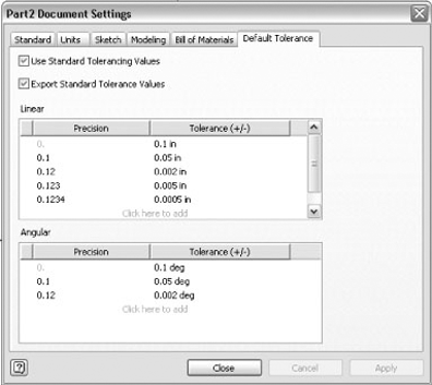
Figure 5.49 shows a simple sketch created using a template setup as described in the previous paragraph. Since the document settings are defaulted to three places, all sketch dimensions are in three places, with the appropriate tolerances. To change the tolerance values of a sketch dimension, simply select the dimension, right-click, and change the precision through the dimension properties of any specific dimension.
The default tolerances are set to +/- tolerances. To select another tolerance standard, simply override the existing tolerance values in the dimension properties or change the precision of a sketch dimension.
You will notice that the global tolerance settings apply tolerances to all dimensions. When a part moves forward into the drawing environment, retrieved dimensions will reflect the nominal value except for dimensions where precision and tolerance are overridden. A better workflow for the drawing environment would be to create multiple dimension styles with various precision and/or tolerance options.
You must keep in mind that the tolerance settings in the part are designed to function with the assembly environment and allow calculating tolerances and stack-ups within the assembly. They are not meant to provide tolerancing in the drawing environment.
Tolerances are an important tool for communicating design intent to manufacturing. Large tolerances indicate that the dimensions aren't critical to the part's function, while tight tolerances indicate that manufacturing needs to pay extra attention to that machining operation. We have fixed a lot of manufacturing problems by changing tolerances. Loosening up tolerances can help manufacturing reduce their reject rate, while tightening up certain tolerances can reduce rework during assembly or in the field.
Tolerances define the acceptable size range for a particular dimension since parts cannot be manufactured to an exact dimension. It is important to set tolerances large enough that parts are economical to manufacture but small enough that the part still functions. Most companies have standard tolerance values for each manufacturing process. For example, weldments usually have large tolerances, while CNC machined parts usually have tighter tolerances. Standard tolerances are usually displayed in the drawing title block and not on the drawing dimensions. If there is a special tolerance, an O-ring groove, for example, then that particular tolerance is displayed on the drawing dimension.
Adding tolerances during the design phase pays dividends down the road. There will be fewer errors creating drawings, and it provides clues to design decisions that are useful when updating an existing part. You might find that using standard tolerances makes the design process more efficient because the designer needs to focus only on the general tolerance for a dimension (two-place vs. three-place tolerance) and apply special tolerances where needed.
Once in a while, even the most skilled design engineer experiences a modeling or design failure. The part may be supplied by a customer or co-worker who has not practiced sound modeling techniques, or you may have to drastically modify a base feature in a part you designed. These edits change a base feature to the point that dependent features cannot solve, and a cascade of errors can occur. Knowing how to fix these errors can save you hours of work
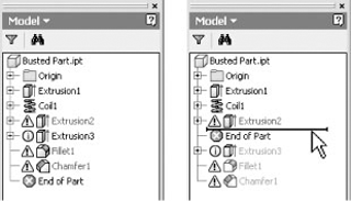
One of the best ways to troubleshoot a part and determine exactly how the part was originally modeled is to use the end-of-part (EOP) marker to step through the creation process. In the Model browser, drag the end-of-part marker to a location immediately below the first feature. This will effectively eliminate all other features below the marker from the part calculation.
Often when making modifications to a part, you might change a feature that causes errors to cascade down through the part. Moving the end-of-part marker up to isolate the first troubled feature allows you to resolve errors one at a time. Oftentimes, resolving the topmost error will fix those that exist after it. Figure 5.50 shows a model tree with a series of errors. On the right, the end-of-part marker has been moved up.
Normally, the first feature will start with a sketch. Right-click the first feature, and select Edit Sketch. Examine the sketch for a location relative to the part origin point. Generally, the first sketch should be located and anchored at the origin and fully dimensioned and constrained. If the sketch is not fully constrained, then add dimensions and constraints to correct it.
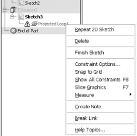
If you see sketch entities highlighted in a magenta color, you probably have projected geometry that has lost its parent feature. To resolve errors of this type, it is often required to break the link between the missing geometry and allow the projected entities to stand on their own. To do so, right-click the objects in the graphics area or expand the sketch in the browser, and right-click and projected or reference geometry that are showing errors; then choose Break Link. This frees up the geometry so that it can be constrained and dimensioned on its own or simply deleted. Figure 5.51 shows the Break Link option being selected for a projected loop.
Once the sketch is free of errors, you can return to the feature level. Often you'll be greeted by an error message informing you that the feature is not healthy. Click Edit or Accept. Then edit the feature. Most often you will simple be required to reselect the profile or reference geometry. Once the feature is fixed, drag the end-of-part marker below the next feature, and repeat the step. Continue through the part until all sketches are properly constrained.
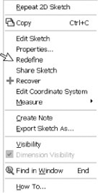
Occasionally, a base sketch may become "lost" and may need to be reassociated to a sketch plane. To do so, you can right-click and choose Redefine, as shown in Figure 5.52. Depending on how drastic the change in sketch plane is, this may be all that is required. Often, though, you will need to edit the sketch, clean up some stray geometry using the Break Link option, and then dimension and constrain it so that it is stable.
Step 2 might be called "learn from your mistakes" (or other people's mistakes). When you have part/feature failures, you should take advantage of them and analyze how the part was created to determine why the sketch or features became unstable. It's always good practice to create the major features first and then add secondary features such as holes, fillets, and chamfers at the end of the part. On occasion, loft and sweep features may fail or produce incorrect results because fillets and chamfers were created before the failed feature. To determine whether this is the case in your model, suppress any holes, fillets, chamfers, or any other feature that you might think is causing the failure.
Once the failed feature is corrected, introduce one suppressed feature at a time until you encounter a failure. This will identify the cause. You may then attempt to move the offending feature below the failed feature and examine the result. If you are unable to move the offending feature, then reproduce the same feature below the failed feature, and leave the original suppressed. When the problems are corrected in a part, you can go back and delete the suppressed offending features.
Although it's not always a silver bullet, you might want to try the Rebuild All tool right after fixing the first broken sketch or feature. Very often if the fix was fairly minor, Rebuild All will save you from having to manually edit dependant features one at a time. You can access this tool by going to the Manage tab and selecting Rebuild All.
- Create complex sweeps and lofts
Complex geometry is created by using multiple work planes, sketches, and 3D sketch geometry. Honing your experience in creating work planes and 3D sketches is paramount to success in creating complex models.
- Master It
How would you create a piece of twisted flat bar in Inventor?
- Work with multi-body and derived parts
Multi-body parts can be used to create part files with features that require precise matching between two or more parts. Once the solid bodies are created, you can create a separate part file for each component.
- Master It
What would be the best way to create an assembly of four parts that require features to mate together in different positions?
- Utilize part tolerances
Dimensional tolerancing of sketches allows the checking of stack-up variations within assemblies. By adding tolerances to critical dimensions within sketches, parts may be adjusted to maximum, minimum, and nominal conditions.
- Master It
You want to create a model feature with a deviation so that you can test the assembly fit at the extreme ends of the tolerances.
- Understand and use parameters and iProperties
Using parameters within files assist in the creation of title blocks, parts lists, and annotation within 2D drawings. Using parameters in an assembly file allows the control of constraints and objects within the assembly. Exporting parameters allows the creation of custom properties. Proper usage of iProperties facilitates the creation of accurate 2D drawings that always reflect the current state of included parts and assemblies.
- Master It
You want to create a formula to determine the spacing of a hole pattern based upon the length of the part.
- Troubleshoot modeling failures
Modeling failures are often caused by poor design practices. Poor sketching techniques, bad design workflow, and other factors can lead to the elimination of design intent within a model.
- Master It
You want to modify a rather complex existing part file, but when you change the feature, errors cascade down through the entire part.