
In This Chapter
Sorting your cases in different ways
Combining counting and case identifying
Recoding variable content to new values
Grouping data in bins
After you get your raw data into SPSS, you may find that it contains errors or that it may not be organized the way you'd like. A way to alleviate these problems is by making modifications to your data configuring the values into a form that's easier to work with and to read. This chapter contains some methods you can use to modify your data without loss of information.
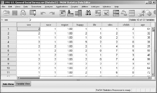
You can change the order of your cases (rows) so they appear in just about any order you want. You sort them by comparing the values you entered for your variables. The following example uses one of the data files that installs with SPSS. The data will be sorted with all males listed first, and with the youngest males first within that sort order. These two variables — in this example, sex and age — are known as the primary and secondary sort keys.
Note
You don't need to limit your sorting to two sort keys. You can have a third and fourth key, if necessary, but these keys come into effect only when the keys sorted before them hold identical values. In most cases, two sort keys are plenty to get what you want.
You can sort based on any variables, of any type, by simply selecting the variables as keys. For example:
From the main menu, choose File
Open Data and load the
1991 U.S. General Social Surveyfile, which is in the PASW directory.The result is the presentation of a collection of apparently unsorted cases shown in Figure 7-1.
From the Data Editor window, choose File
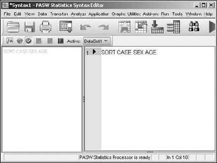
NewSyntax, and the Syntax Editor window appears.In the right panel, to the right of the number 1, enter the four words
SORT CASE SEX AGE. as shown in Figure 7-2.This is one line of Command Syntax language. Be sure to include the period at the end. Although the command will work without it, SPSS will complain.
From the main menu of the Syntax Editor window, choose Run
To End.The Data View window appears as shown in Figure 7-3. The data has been sorted with the male sex — represented by the number 1 — and the youngest age — which is 18 — at the top of the list of cases. It came up male-first because male is defined as 1, which is a smaller number than the 2 that represents female.
To change the order in which things are sorted, replace the command in the Syntax Editor window with
SORT CASE SEX (D) AGE.You can reverse the sort order for any or all variables selected as sort keys. The default is ascending order — smallest to largest — but you can specify descending order by following a variable name with a
(D)indicator. The resulting sort, with the youngest female first, is shown in Figure 7-4.


Note
Sorting data is strictly for the way you want it to appear in the table. The order in which the data is displayed never affects the analysis.
The order of the sort keys is important. In the preceding example, if AGE had been chosen as the first key and SEX as the second, here's how the sort would have run: All 18-year-olds would have come up first in the list, ordered by female and then male. Following that, the next age would have come up, and it too would have been ordered by sex, and so on.
If your data is being used to keep track of multiple similar occurrences — such as people who subscribe to any combination of three different magazines, or eggs produced with something other than a single yolk — you can automatically generate a count of the occurrences for each case. SPSS automates the process of creating a new variable and counting the values for you. You specify what value or values cause a variable to qualify, and SPSS counts the number of qualifying variables from among those you choose. You must have a number of variables that all normally take the same range of values. For example, if you have a number of expenses for each case, you could have SPSS count the number of expenses that exceed a certain threshold.
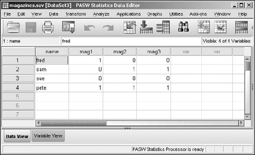
In the following example, people are listed as subscribers or nonsubscribers to three magazines, which are named simply mag1, mag2, and mag3. The following steps generate a total of the number of subscriptions for each person:
Choose Open
FileData and open themagazines.savfile.This file can be downloaded as described in the introduction. The screen shown in Figure 7-5 appears.
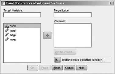
Choose Transform
Count Values Within Cases.The screen shown in Figure 7-6 appears.
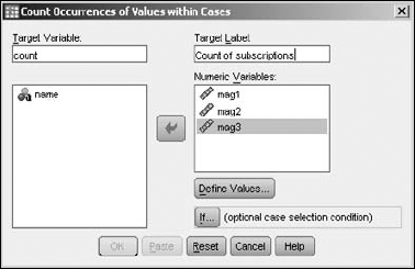
Select the name of every variable you want to use in the count, and then click the arrow to move them from the panel on the left to the panel on the right labeled Variables. Give your new variable a name.
This operation works only with numerics because it must perform numeric matches on the values. If you want, you can come up with both a name and a label to be assigned to the variable that this process creates. In this example, the name is
countand the label isCount of subscriptions, as shown in Figure 7-7.Click the Define Values button.
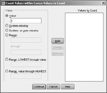
The window shown in Figure 7-8 appears. In this window, I've decided to count, from among the selected variables, those with the numeric value of 1 — which in our example is the value that signifies a subscription.
As you can see in the figure, the total can also be based on missing values and ranges of values. In the ranges, you can specify both the high and low values, or you can specify one end of the range and have the other end be either the largest or the smallest value in the set. In fact, you can select a number of criteria and SPSS will check each variable against all of them.
Select a criterion value you want to use, and then click the Add button to move it to the panel on the right labeled Values to Count. Repeat as needed to define all your criteria.
The new variable will contain a count of the variables that you named that have a value that matches at least one of the criteria you specified. Each case is counted separately.
Click the Continue button.
You return to the Count Occurrences of Values within Cases screen (refer to Figure 7-6).
Click the If button.
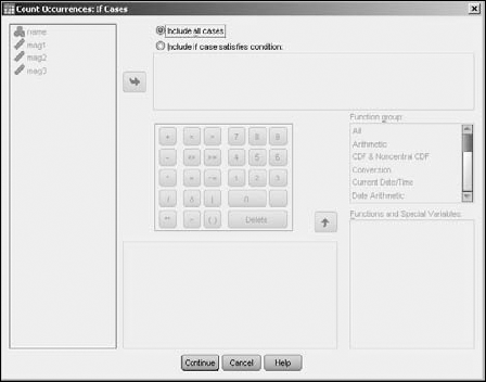
The window shown in Figure 7-9 appears.
Define your expression.
By default, all cases are included, but you can specify criteria here to exclude some cases. To do so, select the Include If Case Satisfies Condition option and, in the text box below, define an expression that specifies the values you want to accept. Then only the values for which the expression is true are considered as candidates for a count greater than 0. You can use any of the variables in the expression. And by using the number pad, the operator buttons, and the function selection, you can construct any expression you want. (For more information on constructing expressions, see Part V.)
Click the Continue button to have SPSS accept your definition. Otherwise (as I did for this simple example), click Cancel and all cases are considered.
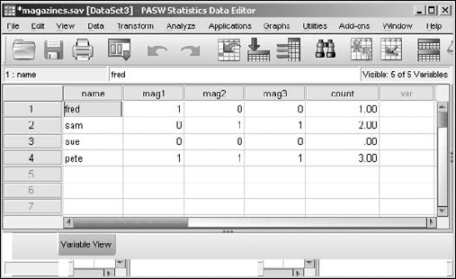
Click the OK button and the new field, along with its counts, is generated.
The result is the new variable named
count, as shown in Figure 7-10.
You can have SPSS change specific values to other specific values according to rules you give it. You can change almost any value to anything else. For example, if you have yes and no represented by 5 and 6, you could recode the values into 1 and 2. You can recode the values in place without creating a new variable, or you can create a new variable and recode values into it. You may want to do this to correct errors or to make the data easier to use.
Warning
When you're recoding values without creating a new variable to receive the new numbers, be sure you store a safety copy of your data before you start. Changes to your data can't be automatically reversed; you could destroy information.
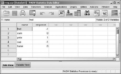
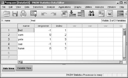
The following example is a list of names of individuals who were invited to an event. If they responded with a yes, the response value was set to 1; if they responded with a no, the value was set to −1. Those with a 0 have not yet responded. As the date of the event approaches, you decide to convert all the −1 responses to 0 to get a count of people not coming. Here's how.
To download the file, go to this book's Web site. You can download this single file or all the files created for this book. Simply place the files in a directory where you can find them through the menus of SPSS. Then follow these steps:
Choose Open
File and load thersvp.savfile.The window shown in Figure 7-11 appears.
Choose Transform
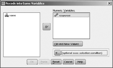
Recode into Same Variables.Select the
responsevariable and click the button with the arrow to move the variable to the panel on the right, labeled Numeric Variables, as shown in Figure 7-12.Click the Old and New Values button.
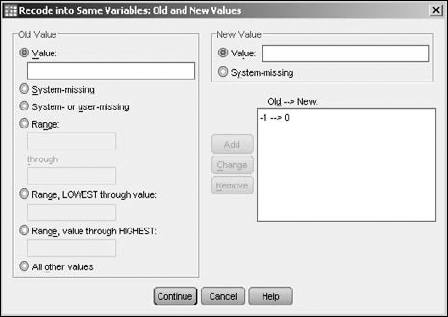
The window shown in Figure 7-13 appears.
As shown in the figure, enter an existing value in one of the Old Value choices, and then enter a New Value for it.
You can specify a range of old values and map them to a new value. You can also specify that the new value is to be missing and the old value will be mapped to that. You can, if you want, map a number of old values to new values and SPSS will do all the recodings at once. For each mapping of an old value to a new value, use the Add button to make the mapping appear in the window labeled Old-->New.
After you've entered all the mappings (in this example it's just the one), click Continue.
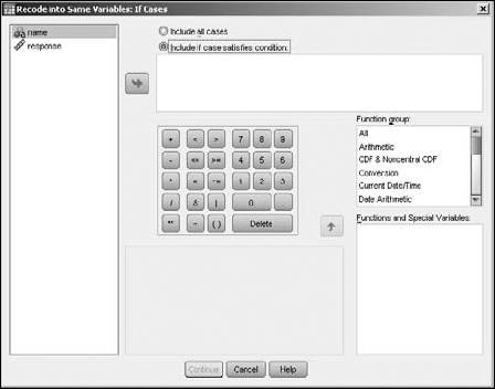
Optionally, rather than clicking the Old and New Values button as in Step 4, you can click the If button and the window in Figure 7-14 appears, so you can limit the number of cases to which the recoding will apply.
You accomplish the limiting by entering an expression that must be true for a case to be included. In our example, we enter no expression, because we want the process to apply to all cases. (For more on expressions, see Part V.)
Click the OK button.
All the −1 values are converted to 0, as shown in Figure 7-15. The variable has had its values recoded.

It could be that you don't want to overwrite the existing values but you'd like to have the recoded data available. The following steps do much the same thing as the preceding example, except the recoded values are stored in a new variable:
With the
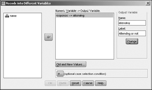
rsvp.savfile loaded the same as before (refer to Figure 7-11), choose TransformRecode into Different Variables.In the left panel, select the variable holding the values you wish to change. Using the arrow in the center, move the variable name to the panel in the center.
On the right, in the Output Variable area, enter a name and label for a new variable.
For the output variable, you can choose a new variable name (so a new variable is created) or choose an existing variable name and have its values overwritten.
Click the Change button and the output variable is defined, as shown in Figure 7-16.
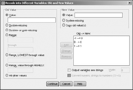
Click the Old and New Values button.
Define the recoding.
Enter an existing value into the Old Value text box and the value you want it to become in the New Value text box. Then click the Add button to add them to the Old-->New list (as shown in Figure 7-17). Be sure to map all values — even the ones that don't change — because you're creating a new variable and it has no preset values.
Click the Continue button.
Click the OK button.
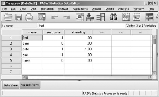
The results appear, as shown in Figure 7-18. Notice that the numbers all have two digits to the right of the decimal point. This may or may not be what you want, but the new variable was created automatically and that is part of the default.
Automatic recoding converts values into something you can use in computations. For example, if you have a list of automobile names, automatic recoding converts those names into numbers so you can perform an analysis on the pattern of numbers. Automatic recoding gives you a numeric handle on data that could otherwise elude analysis.
To perform automatic recoding, you select options and set the names in a single dialog box. To see an example of automatic recoding in operation, follow these steps:
Load
rsvp.sav(refer to Figure 7-11).Choose Transform
Automatic Recode.In the panel on the left, select the name of the variable you want to recode. Then click the arrow in the middle to move the variable to the panel on the right.
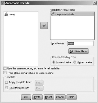
In the New Name text box, enter the name of the variable to receive the recoded values.
Click the Add New Name button.
The name you entered appears in the panel above the new name, as shown in Figure 7-19.
Click the OK button and recoding takes place.
The result is similar to that shown in Figure 7-20, where the new variable is named
index.
The values in the new variable, index, come about from sorting the values of the original variable and then assigning numbers to them in that order. If the input values are a string of characters instead of the digits of numbers, the strings are sorted alphabetically. (Well, almost: Uppercase letters come before lowercase.)
In the Automatic Recode window (refer to Figure 7-19), you can see the choice for recoding the values with new numbers that start with either the lowest or the highest value. The new numeric values will be the same either way; they're just assigned in the opposite order.
At the bottom of the Automatic Recode window are two choices for the creation of a template file. This is so you can save a file — called a Template file — that holds a record of the recoding patterns. That way, if you need to recode more data with the same variable names, the new input values will be compared against the previous encoding and be given appropriate values so that the two data files can be merged and the data will all fit. For example, if you have brand names or part numbers in your data, the recoding will be consistent with the original values because it will be assigned the same pattern of recoded values.
If you're using a scale variable that contains a range of values, you can create groups of those values and organize them into bins. For example, you could use the ages of a number of people and put each one in its own bin — one bin for ages 0 to 20, another bin for 21 to 40, and so on. You can specify the size and content of bins in several ways. The actual binning process is automatic.
The following steps take you through an example of the binning process by dividing salaries into bins:
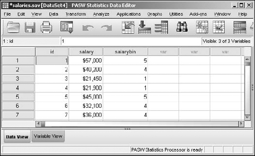
Choose File
OpenData and load thesalaries.savfile.This file is available for download as described in the introduction. This file contains a list of ID numbers with a salary for each one, as shown in Figure 7-21.
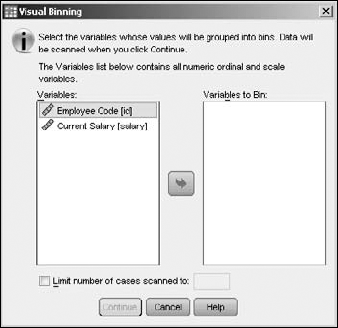
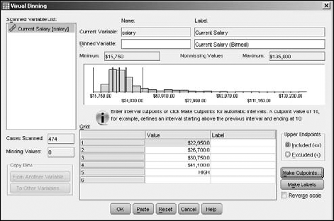
Choose Transform
Visual Binning.The dialog box shown in Figure 7-22 appears.
Select Current Salary in the panel on the left, then click the arrow in the center of the window to move the name of the variable to the panel on the right.
Click the Continue button.
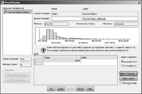
A bar graph displaying the range of values of the salaries appears in the center, as shown in Figure 7-23.
Click the Make Cutpoints button.
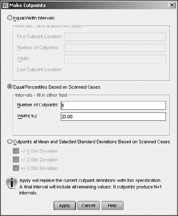
A dialog box appears; here you can specify the size of each bin and the number of bins.
Select the points at which you want to have the data cut into parts to create the bins.
In this example, I divided the data into even percentiles of numbers of cases — that is, each bin will contain the same number of cases, as shown in Figure 7-24. Notice that four cutpoints divide the data into five bins, each holding 20 percent of the cases. I could have chosen to divide the data into equal-width intervals — that is, each bin would contain a range of the same magnitude, which would put different numbers of cases in each bin. Also, the cutpoints could have been based on standard deviations, which would create two cutpoints, dividing the data into the three bins — one each of low, medium, and high capacity.
Click the Apply button, and the cutpoints appear as vertical lines on the bar graph, as shown in Figure 7-25.
You may click the Make Cutpoints button repeatedly and cut the data different ways until you get the cutpoints the way you like. Any new cutpoints you define replace any previous ones.
Enter a name for a new variable to contain the binning information.
You enter the name in the Binned Variable text box. The default label for the new variable appears in the text box to the right of the name. You can change this if you want. The bins are created and numbered from 1 to 5, but if you select the Reverse Scale option (in the lower-right corner), the numbering will be from 5 to 1.
Click OK.
The new variable is created and filled with the bin values, as shown in Figure 7-26.

The binning is now complete and you can use the new data for further analysis. One thing you can do quickly and easily is display a summary of the contents of your bins. Simply follow these steps:
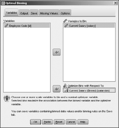
With the window in Figure 7-26 still on the screen, choose Transform
Optimal Binning.Select variable names on the left and click the arrow buttons to move the variables. Move Current Salary to Variables to Bin and move Current Salary (binned) to Optimize Bins with Respect To, as shown in Figure 7-27.
The variable in the Optimize Bins with Respect To text box does not have be a variable from a previous binning operation. It can be any variable that contains a collection of values sufficient for being separated into bins.
Click the OK button.
The output is generated, as shown in Figure 7-28.
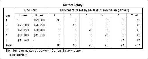
Any variable with properly distributed values can be used as the basis of optimal binning. In the chart shown in Figure 7-28, the numbers 1 through 5 across the top are the values of the new binning variable created and stored as part of the data. The numbers 1 through 5 down the left of the graph are the result of the new binning action. The chart lets you see clearly the range of values that make up each bin.