
6.6. Modeling Relationships
In initial brainstorming sessions to identify causes of bad parts, the team identified five possible Hot Xs:
Coating variables: Anodize Temperature, Anodize Time, and Acid Concentration.
Dye variables: Dye Concentration and Dye pH.
It is time to determine whether these are truly Hot Xs, and to model the relationships that link Thickness, L*, a*, and b* and these Xs. So, Sean will guide the team in conducting a designed experiment. These five process factors may or may not exert a causal influence. The designed experiment will indicate whether they do and, if so, will allow the team to model the Ys as functions of the Xs. The team will use these models to optimize the settings of the input variables in order to maximize yield.
Although Color Rating is the variable that ultimately defines yield, Sean knows that using a nominal response in a designed experiment is problematic—a large number of trials would be required in order to establish statistical significance. Fortunately, the team has learned that there are strong relationships between Thickness, L*, a*, and b, and the levels of Color Rating. Accordingly, Sean and his team decide that the four responses will be L*, a*, b*, and Thickness. There will be five factors: Anodize Temp, Anodize Time, Acid Conc, Dye Conc, and Dye pH.
With the data from this experiment in hand, Sean plans to move to the Model Relationships phase of the Visual Six Sigma Data Analysis Process (Exhibit 3.29). He will use the guidance given under Model Relationships in the Visual Six Sigma Roadmap (Exhibit 3.30) to direct his analysis.
6.6.1. Developing the Design
The team now faces a dilemma in terms of designing the experiment, which must be performed on production equipment. Due to the poor yields of the current process, the equipment is in continual use by manufacturing. Negotiating with the production superintendent, Sean secures the equipment for two consecutive production shifts, during which the team will be allowed to perform the experiment. Since the in-process parts, even prior to anodizing, have high value, and all the more so given the poor yields, the team needs to use as few parts as possible in the experiment. Given these practical considerations, the team determines that at most 12 experimental trials can be performed and decides to run a single part at each of these experimental settings.
Sean points out to the team members that if they employ a two-level factorial treatment structure for the five factors (a 25 design), 32 runs will be required. Obviously, the size of the experiment needs to be reduced. Sean asks for a little time during which he will consider various options.
Sean's first thought is to perform a 25–2 fractional factorial experiment, which is a quarter fraction of the full factorial experiment. With the addition of two center runs, this experiment would have a total of ten runs. However, Sean realizes, with the help of the JMP Screening Design platform (DOE > Screening Design), that the 25–2 fractional factorial is a resolution III design, which means that some main effects are aliased with two-way interactions. In fact, for this particular design, each main effect is aliased with a two-way interaction.
Sean discusses this idea with the team members, but they decide that it is quite possible that there are two-way interactions among the five factors. They determine that a resolution III fractional factorial design is not the best choice here. As Sean also points out, for five experimental factors there are ten two-way interaction terms. Along with the five main effects, the team would need at least 16 trials to estimate all possible two-way interactions, the main effects, and the intercept of the statistical model. However, due to the operational constraints this is not possible, so the team decides to continue the discussion with two experts, who join the team temporarily.
Recall that the anodize process occurs in two steps:
Step 1 The anodize coating is applied.
Step 2 The coated parts are dyed in a separate tank.
The two experts maintain that interactions cannot occur between the two dye tank factors and the three anodize tank factors, although two-way interactions can certainly occur among the factors within each of the two steps. If the team does not estimate interactions between the factors in each of the two anodize process steps, only four two-way interactions need to be estimated:
Anodize Temperature*Anodize Time
Anodize Temperature*Acid Concentration
Anodize Time*Acid Concentration
Dye Concentration*Dye pH
So with only ten trials, it will be possible to estimate the five main effects, the four two-way interactions of importance, and the intercept. This design is now feasible. Sean and his teammates are reasonably comfortable proceeding under the experts' assumption, realizing that any proposed solution will be verified using confirmation trials before it is adopted.
Another critical piece of knowledge relative to designing the experiment involves the actual factors settings to be used. With the help of the two experts that the team has commandeered, low and high levels for the five factors are specified. The team members are careful to ensure that these levels are aggressive relative to the production settings. Their thinking is that if a factor or interaction has an effect, they want to maximize the chance that they will detect it.
Sean now proceeds to design the experiment. He realizes that the design requirements cannot be met using a classical design. Fortunately, he knows about the Custom Design platform in JMP (DOE > Custom Design). The Custom Design platform allows the user to specify a constraint on the total possible number of trials and to specify the effects to be estimated. The platform then searches for optimal designs (using either the D- or I-optimality criterion) that satisfy the user's requirements.
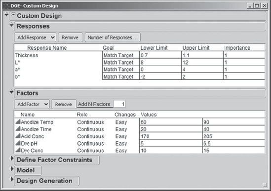
Sean selects DOE > Custom Design and adds the responses and factors as shown in Exhibit 6.40. Note that the four Ys are entered in the Responses panel, along with their response limits (Lower Limit, Upper Limit), which Sean sets to the specification limits. For each response, the goal is to match the target value, so Sean leaves Goal set at March Target. (JMP defines the target value to be the midpoint of the response limits.) Sean retains the default Importance value of 1, because he currently has no reason to think that any one response is of greater importance than another in obtaining good color quality. Sean also specifies the five factors and their low and high levels in the Factors panel.
Figure 6.40. Custom Design Dialog Showing Responses and Factors
In the menu obtained by clicking on the red triangle, Sean finds the option to Save Responses and Save Factors, and he does so for future reference. JMP saves these simply as data tables. (If you don't want to enter this information manually, click on the red triangle to Load Responses and Load Factors. The files are Anodize_CustomDesign_Responses.jmp and Anodize_CustomDesign_Factors.jmp.)
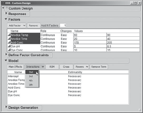
Initially, the Model panel shows the list of main effects. To add the desired two-way interactions, while holding the shift key, Sean selects the three anodize factors, Anodize Temp, Anodize Time, and Acid Conc, in the list of Factors. Then, he clicks on Interactions in the Model panel, selecting 2nd. This is illustrated in Exhibit 6.41. This adds the three interactions to the Model panel. Sean adds the single Dye pH*Dye Conc interaction in a similar fashion.
Figure 6.41. Adding the Anodize Interactions to the Model List
In the Design Generation panel, Sean specifies 10 runs (next to User Specified). He wants to reserve 2 of his 12 runs for center points. The completed dialog is shown in Exhibit 6.42.
Figure 6.42. Completed Dialog Showing Custom Design Settings

When Sean clicks Make Design, JMP constructs the requested design, showing it in the Custom Design dialog. Sean's design is shown in Exhibit 6.43. The design that you obtain will very likely differ from this one. This is because the algorithm used to construct custom designs involves a random starting point. The random seed changes each time you run the algorithm. To obtain the same design every time, you can set the random seed, selecting Set Random Seed from the red triangle menu. (For Sean's design, the random seed is 31675436.)
Sean inspects his design (Exhibit 6.43) and finds that it makes sense. He examines the Output Options panel and agrees with the default that the Run Order be randomized. He specifies 2 as the Number of Center Points, including these to estimate pure error and to check for lack of fit of the statistical models. Then he clicks Make Table.
Figure 6.43. Custom Design Runs and Output Options

The data table generated by JMP for Sean's design is called Anodize_CustomDesign_Table.jmp and is shown in Exhibit 6.44. Note that two center points have been specified; these appear in the randomization as trials 3 and 8. Sean and the team are delighted to see that JMP has saved the script for the model that the team will eventually fit to the data. It is called Model and is located in the table panel in the upper left corner of the data table. This script defines the model that Sean specified when he built the design, namely, a model with five main effects and four two-way interactions. (To see this, run the script.)
Figure 6.44. Design Table Generated by Custom Design
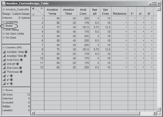
Sean notices that JMP has saved two other scripts to this data table. One of these scripts, Screening, runs a screening analysis. In this analysis, a saturated model is fit. Sean will not be interested in this analysis, since he has some prior knowledge of the appropriate model. The other script, DOE Dialog, reproduces the DOE > Custom Design dialog used to obtain this design.
Sean also notices the asterisks next to the variable names in the columns panel (Exhibit 6.45). He clicks on these to learn that JMP has saved a number of Column Properties for each of the factors: Coding, Design Role, and Factor Changes. Clicking on any one of these takes Sean directly to that property in Column Info. Similarly, for each response, Response Limits has been saved as a Column Property.
Figure 6.45. Column Properties for Anodize Temp

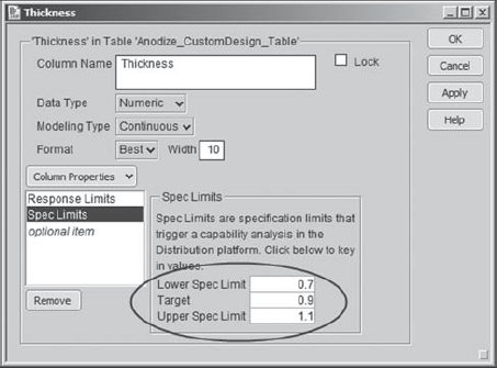
Sean decides to add each response's specification limits as a column property. He believes this information will be useful later, when determining optimal settings for the factors. To set specification limits for Thickness, Sean right-clicks in the header for the Thickness column. From the menu that appears, he chooses Column Info. In the Column Info window, from the Column Properties list, Sean selects Spec Limits. He populates the Spec Limits box as shown in Exhibit 6.46.
Figure 6.46. Dialog for Thickness Spec Limits
In a similar fashion, Sean saves Spec Limits as a column property for each of L*, a*, and b*. These will be useful later on. (The script Set Spec Limits will set the specification limits for all four responses at once.)
6.6.2. Conducting the Experiment
The team is now ready to perform the experiment. Sean explains the importance of following the randomization order and of resetting all experimental conditions between runs. The team appreciates the importance of these procedures and plans the details of how the experiment will be conducted. The team also decides to number the parts in order to mistake-proof the process of taking measurements.
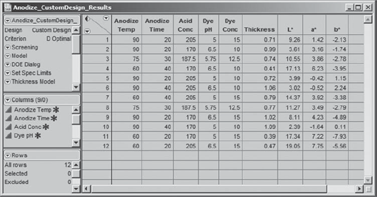
The team members proceed to conduct the experiment. The design and measured responses are given in the data table Anodize_CustomDesign_Results.jmp (Exhibit 6.47).
Figure 6.47. Results of Designed Experiment
6.6.3. Uncovering the Hot Xs
It is time to analyze the data, and Sean and the team are very excited! Sean will attempt to identify significant factors by modeling each response separately, using the Fit Model platform. For each of the four responses, Sean follows this strategy:
Examine the data for outliers and possible lack of fit, using the Actual by Predicted plot as a visual guide. Check the Lack Of Fit Test, which can be conducted thanks to the two center points, in order to confirm his visual assessment of the Actual by Predicted plot.
Find a best model by eliminating effects that appear insignificant.
Save the prediction formula for the best model as a column in the data table.
Save the script for the best model to the data table for future reference.
Sean's plan, once this work is completed, is to use the Profiler to find factor level settings that will simultaneously optimize all four responses.
Sean runs the Model script saved in the table information panel. This will fit models to all four responses. But Sean wants to examine these one by one, starting with the model for Thickness. So he removes the other three responses from the Fit Model dialog by selecting them in the Y text box and clicking the Remove button.
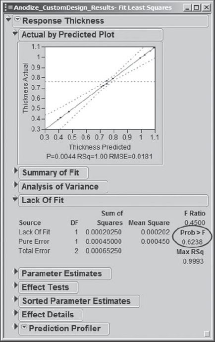
Then Sean clicks Run Model to run the full model for Thickness. In the report, from the red triangle drop-down menu, he chooses Row Diagnostics > Plot Actual by Predicted. The report for the model fit to Thickness, shown in Exhibit 6.48, shows no significant lack of fit—both the Actual by Predicted plot and the formal Lack Of Fit test support this conclusion (the p-value for the Lack of Fit test is Prob > F = 0.6238). Note that this is a nice example of Exploratory Data Analysis (the Actual by Predicted plot) being reinforced by Confirmatory Data Analysis (the Lack Of Fit test).
Figure 6.48. Report for Full Model for Thickness
Since the model appears to fit, Sean checks the Analysis of Variance panel and sees that the overall model is significant (Exhibit 6.49). He knows that he could examine the Effect Tests table to see which effects are significant. However, he finds it easier to interpret the Sorted Parameter Estimates table (Exhibit 6.49), which gives a graph where the size of a bar is proportional to the size of the corresponding effect. He examines the Prob > |t| values, and sees that two of the two-way interactions, Anodize Temp*Anodize Time and Dye pH*Dye Conc, do not appear to be significant (Sean decides that a significant p-value is one that is less than 0.05).
Figure 6.49. ANOVA and Sorted Parameter Estimates for Full Model for Thickness

At this point, Sean can opt for one of two approaches. He can reduce the model manually or he can use a stepwise procedure. In the past, he has done model reduction manually, but he has learned that JMP has a Stepwise platform that allows him to remove effects from a model for a designed experiment in a way that is consistent with the hierarchy of terms. So he tries both approaches.
In the manual approach, Sean removes the least significant of the two interaction terms from the model, namely, Dye pH*Dye Conc. The Fit Model dialog remains open, and so it is easy to remove this term from the Model Effects box. He refits the model without this term, notes that Dye Conc is the next least significant term, removes it, and refits the model. Next, each in turn, Dye pH and Anodize Temp*Anodize Time are removed from the model. At this point, all remaining terms are significant at the 0.05 level (Exhibit 6.50).
Figure 6.50. Fit Least Squares Report for Reduced Thickness Model

In the stepwise approach, Sean asks JMP to reduce the model exactly as he has just reduced it. He needs to rerun the full model for Thickness, since he was modifying the Fit Model dialog just now. He reruns the script Model and removes the other three responses, since model reduction is only done for one response at a time. Under Personality, he chooses Stepwise, as shown in Exhibit 6.51.
Figure 6.51. Selection of Stepwise Regression from Fit Model Dialog

When Sean clicks Run Model, the Fit Stepwise dialog box opens. He clicks on Enter All to enter all effects into the model. Then he sets up the dialog options as shown in Exhibit 6.52: He sets Prob to Leave to 0.05, so that effects will be removed if their p-values exceed 0.05; he sets the Direction to Backward, so that effects are removed in turn (and effects are not entered); and he chooses Restrict under Rules. This last choice removes effects in a fashion consistent with the hierarchy of terms. For example, a main effect is not removed so long as an interaction involving the main effect is significant.
Figure 6.52. Fit Stepwise Dialog Settings for Thickness Model Reduction
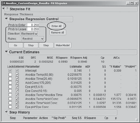
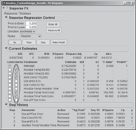
At this point, Sean can click Step to view the removal of terms one by one, or he can click Go to have the reduction done all at once. Either way, the procedure ends with four effects removed, as shown in Exhibit 6.53.
Figure 6.53. Results of Stepwise Reduction for Thickness
Now, in the Fit Stepwise dialog, Sean clicks Make Model. This creates a Stepped Model dialog to fit the reduced model (Exhibit 6.54). He notes that this is the same model that he obtained using the manual approach.
Figure 6.54. Stepped Model Dialog for Reduced Model for Thickness

Sean observes that these are precisely the significant effects left in the model that he reduced manually, whose analysis is shown in Exhibit 6.50. He adopts this as his reduced and final model for Thickness.
Sean notices that the final Thickness model contains two significant interactions. He also notes that only factors in the anodizing step of the process are significant for Thickness. Thus, the team finds that the model is in good agreement with engineering knowledge, which indicates that factors in the dye step should not have an impact on anodize thickness. Sean saves a script that creates the fit model dialog for his final Thickness model to the data table as Thickness Model.
Sean uses the stepwise approach in a similar fashion to determine final models for each of the other three responses. These models are also saved to the table information panel in the data table Anodize_CustomDesign_Results.jmp (see Exhibit 6.55). Each of the models for L*, a*, and b* includes factors from both the anodizing and dyeing processes.
Figure 6.55. Final Model Scripts for Four Responses
