You use Excel, of course, to make a spreadsheet—an electronic ledger book composed of rectangles, known as cells, laid out in a grid (see Figure 12-1). As you type numbers into the rectangular cells, the program can automatically perform any number of calculations on them. And although the spreadsheet’s forte is working with numbers, you can use them for text, too; because they’re actually a specialized database, you can turn spreadsheets into schedules, calendars, wedding registries, address books, and other simple text databases.
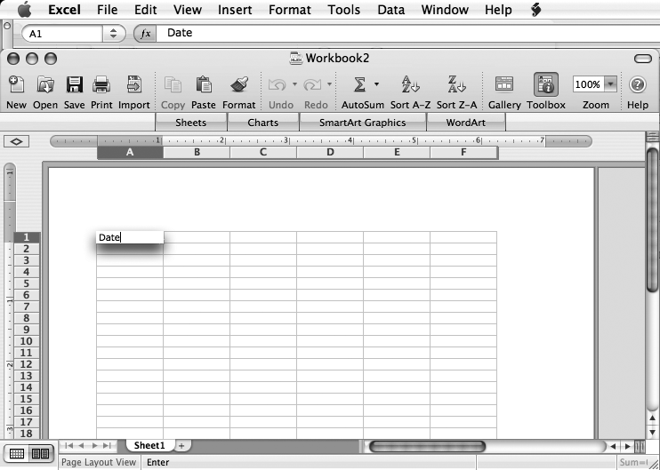
Figure 12-1. Excel 2008 has all the usual Mac OS X doodads, like close, minimize, and zoom buttons and a status bar. In the status area at the bottom left, Excel tells you what it thinks is happening—in this case, Enter indicates the active cell (A1) is being edited.
A new Excel document, called a workbook, is made up of one or more pages called worksheets. (You’ll find more on the workbook/worksheet distinction in Chapter 14.) Each worksheet is an individual spreadsheet, with lettered columns and numbered rows providing coordinates to refer to the cells in the grid.
You can create a plain-Jane Excel workbook by selecting File → New Workbook (⌘-N), or you can use the Office Project Gallery (File → Project Gallery). If you happen to find a template that fits what you’re trying to do, like planning a budget, the Gallery can be a real timesaver. For even more timesavings, check out Excel 2008’s new Ledger Sheets category, a collection of preformatted ledger templates for a variety of common list and financial tasks—with formulas already calculated for you. You can choose from address lists, gift lists, check registers, budgets, invoices, expense reports, portfolio trackers, and lots more.
Tip
Once you’ve added a Ledger Sheet, you can use it as-is or customize any part of it. Even without any spreadsheet skills, you can start filling in these preformatted sheets without having to think about cell formatting, cell references, or formulae—and still take advantage of Excel’s data- and number-crunching prowess. (But you’ll still find this chapter helpful when it comes time to customize a ledger sheet—or if you’re interested in how it’s doing what it does.)
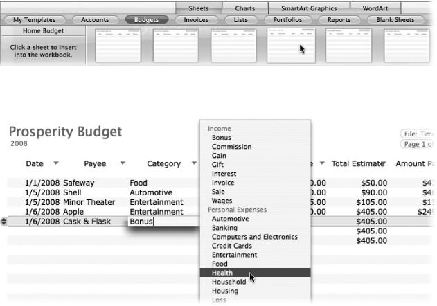
Figure 12-2. Top: You can quickly add a ledger sheet to an Excel workbook by clicking the Elements Gallery’s Sheets tab and clicking one of the Ledger Sheet category buttons. As you move your cursor over the thumbnails, the sheet title appears at the left; click a thumbnail to add the sheet to your workbook. Start typing to enter your data, and use Tab or Return to move to the next column. Bottom: Some columns (such as Category) feature a gray triangle, click it to choose an entry from a pop-up menu. (Ledger Sheets are actually lists, which are described starting on Excel, the List Maker.)
Whether it stars out plain or preformatted, each worksheet can grow to huge proportions—about 16,000 columns wide (labeled A, B, C… AA, AB, AC… AAA, AAB, AAC, and so on, and on, and on), and one million rows tall (see Figure 12-3). Furthermore, you can get at even more cells by adding more worksheets to the workbook by clicking the plus-sign button next to the worksheet tabs at the bottom left or by choosing Insert → Worksheet. Switch between worksheets by clicking their tabs.
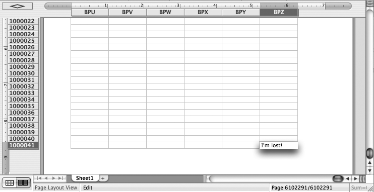
Figure 12-3. You can’t scroll all the way to cell BPZ10000041 in a new spreadsheet (well, you can, but it may take several days), but you can leap to that fardistant cell by typing BPZ10000041 in the Name box on the left side of the Formula bar and pressing Return.
In total, you can have 17.18 billion cells in a single Excel worksheet (16,384 columns x 1,048,576 rows = 17,179,869,184 cells, to be precise). The only company that needs more space than that for its accounting is Microsoft itself.
Tip
Newly minted worksheets always bear the name Sheet1, Sheet2, and so on. To rename a worksheet, double-click the sheet’s name (it’s on the tab on the bottom) and type in a new one. Sheet names can be as long as 31 characters.
Each cell acts as a container for one of two things: data or a formula. Data can be text, a number, a date, or just about anything else you can type. A formula, on the other hand, does something with the data in other cells—such as adding together the numbers in them—and displays the result. (There’s more on formulas later in this chapter.)
Excel refers to cells by their coordinates, such as B23 (column B, row 23). A new spreadsheet has cell A1 selected (surrounded by a thick border)—it’s the active cell. When you start typing, the cell pops up slightly, apparently hovering a quarter-inch above your screen’s surface, with a slight shadow behind it. Whatever you type appears in both the active cell and the Edit box on the right side of the Formula bar. If you prefer, you can click in the Formula bar and do your typing there. When you finish typing, you can do any of the following to make the active cell’s new contents stick:
Press Return, Tab, Enter, or an arrow key.
Click another cell.
Click the Enter button in the Formula bar.
Tip
When you enter information into a cell by pasting, you may see a smart button pop up in the immediate vicinity (Figure 12-4). Clicking the button’s arrow reveals a contextual menu with a number of formatting options specific to the information you’re pasting and where you’re pasting it.
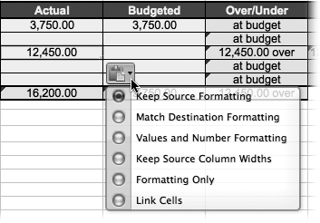
Figure 12-4. A smart button often appears just after you paste data into a cell. Click its arrow to display a small pop-up menu from which you can choose to retain the source formatting (so that the text will retain the formatting it had in its original location or document) or match the destination formatting (in which Excel automatically adjusts the text to the formatting in the current workbook). Variations include pasting just the values and number formatting, pasting the source column width, pasting just the cell formatting, and creating a link to the source cell (see Iterations). Since Excel isn’t psychic, the smart button gives you a chance to tell it whether you had the old or new formatting in mind.
Working in an Excel sheet is simple, at its heart: You enter data or a formula into a cell, move to the next cell, enter more information, and so on. But before entering data in a cell, you have to first select the cell. Clicking is the easiest method; after you click a cell, the cell border thickens and as soon as you start typing, the cell does that popping-up thing.
Tip
When you double-click a cell, it pops up from the spreadsheet and you find yourself again in the editing mode. If, perhaps due to an over-eager mouse-button finger, you keep landing in this “in-cell editing” mode accidentally, choose Excel → Preferences → Edit panel, turn off “Double-click allows editing directly in the cell,” and click OK. Now you can only edit cell contents in the Edit box on the Formula Bar.
To select a cell far away from the current active cell, enter the cell’s address (the column letter followed by the row number) in the Name box on the Formula bar and press Return (see Figure 12-3). Or choose Edit → Go To (or press F5), to summon a dialog box where you can enter the address of the lucky cell in the Reference field.
But the fastest means of getting from cell to cell is to use the keyboard. Excel is loaded with keyboard shortcuts that make it easy to plow through an entire sheet’s worth of cells without having to touch the mouse. Here’s the cheat sheet:
Tip
Return doesn’t have to select the next cell down; it can select any of the four neighboring cells, or do nothing at all. You change what the Return key does in the Excel → Preferences → Edit panel.
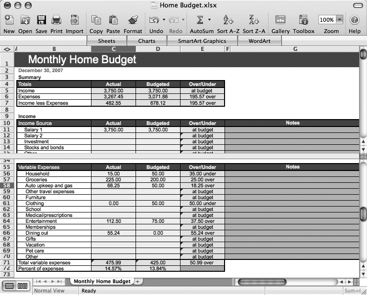
Figure 12-5. Double-click or drag the horizontal or vertical split boxes to simultaneously view two or four parts of a large spreadsheet in one window. Double-click the bar between panes to remove the split view.
Excel is positively brimming with keyboard shortcuts—the table on Data Entry is just the tip of the iceberg. For a complete list, open Excel Help and search for “Excel keyboard shortcuts.” (By not including the entire list in this book, we’re saving a small forest somewhere in Oregon.)
You can enter four kinds of data into an Excel spreadsheet: numbers, text, dates, or times (not including formulas, which are described beginning on Formula Fundamentals). Mostly, entering data is as straightforward as typing, but exceptions lurk.
There are only 21 characters that Excel considers numbers or parts of numbers: 1 2 3 4 5 6 7 8 9 0 . , () + - / $ % e and E. Anything else is treated as text, which is ineligible for performing most calculations. For example, if Excel sees threein a cell, it sees a bunch of typed characters with no numerical value; when it sees 3.14, it sees a number.
Depending on the formatting of the cell where you’re entering numbers, Excel might try to do some work for you. For example, if you’ve applied currency formatting to a cell, Excel turns 3/2 into $1.50. But if you’ve formatted the same cell as a Date, Time, or General, Excel turns 3/2 into a date—March 2 of the current year.
When you’ve formatted a cell to accept General input, and the number you’ve entered is longer than 11 digits (such as 12345678901112), Excel converts it to scientific notation (1.23457E+13).
Excel’s number precision is 15 significant digits—anything over 15 will be lost.
Text can be any combination of characters: numbers, letters, or other symbols.
To make Excel look at a number as if it were a string of text (rather than a number with which it can do all kinds of mathematical wizardry), you have to either precede the number with an apostrophe or format the cell as a text-based cell. To format the cell, choose Text from the Format menu in the Formatting Palette’s Number pane. Alternatively, select the cell and choose Format → Cells (or right-click the cell and choose Format Cells from the shortcut menu). Click the Number tab and then select Text from the Category list. Click OK.
You can perform math on dates, just as though they were numbers. The trick is to type an equal sign (=) into the cell that will contain the answer; then enclose the dates in quotation marks and put the operator (like + or *) between them. For example, if you click a cell, type = “12/30/2007"-"5/25/1963”, and then press Enter, Excel fills the cell with 16290, the number of days between the two dates.
Tip
If you’re trying to determine someone’s age with this calculation, you probably want to write it as =(“12/30/2007” -"5/25/1963”)/365 which gives a result in years: 44.63013699.
This math is made possible by the fact that dates in Excel are numbers. Behind the scenes, Excel converts any date you type into a special date serial number, which is composed of a number to the left side of a decimal point (the number of days since January 1, 1904) and a number on the right (the fraction of a day).
When entering dates, you can use either a slash or a hyphen to separate months, days, and years. Usually it’s OK to format date and time numbering at any time. However, you’ll avoid occasional date recognition problems by applying date or time formatting before you enter the data in the cell.
Excel also treats times as numbers—specifically, as the fractional part of a date serial number, which is a number representing the number of days since midnight on January 1, 1904.
Excel bases times on the 24-hour clock, or military time. To enter a time using the 12-hour clock, follow the number with an a or p. For example, to Excel, 9:34 always means 9:34 a.m., but 9:34 p means 9:34 p.m.—and 21:34 also means 9:34 p.m. Whether you type 9:34 p or 21:34, Excel displays it in the spreadsheet as 21:34 unless you format the cell to display it in the AM/PM format.
As with dates, you can perform calculations on times by entering an equal sign and then enclosing the times in quotation marks and typing the separator in the middle. For example, = “9:34"-"2:43” gives you 0.285416667, the decimal fraction of a day between 2:43 a.m. and 9:34 a.m. If you format the cell with time formatting, as described on Adding number formats, you instead get a more useful 6:51, or six hours and 51 minutes’ difference.
Note
If the times in a calculation span midnight, the calculation will be wrong, since times reset at midnight. Fix it by adding 24 hours to the calculation—or even better by using the MOD function. (See Functions for more on functions.)
Excel 2008 is teeming with features to save you typing. The first, AutoComplete, comes into play when you enter repetitive data down a column. Find out more in Figure 12-6.
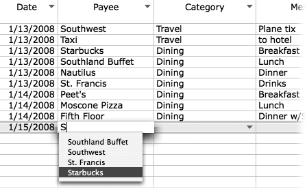
Figure 12-6. Excel’s AutoComplete function watches as you type in a given cell. If your entry looks as though it might match the contents of another cell in the same column, Excel shows a pop-up menu of those possibilities. To select one, press the down arrow until the entry you want is highlighted, and then press Return. Alternatively, just click the entry in the list. Either way, Excel finishes the typing work for you.
Formula AutoComplete is a new feature appearing in Excel 2008, extending the AutoComplete concept to the chore of writing formulas. Instead of having to remember all the elements for a formula, Excel prompts you with valid function names and syntax as you type .
Excel’s AutoFill feature can save you hours of typing and possibly carpel tunnel surgery, thanks to its ingenious ability to fill miles of cells with data automatically. The Edit → Fill submenu is especially useful when you’re duplicating data or typing items in a series (such as days of the week, months of the year, or even sequential apartment numbers). It has seven options: Down, Right, Up, Left, Across Sheets, Series, and Justify.
Here’s how they work. In each case, you start the process by typing data into a cell and then highlighting a block of cells beginning with that cell (see Figure 12-7). Then, choose any of the following:
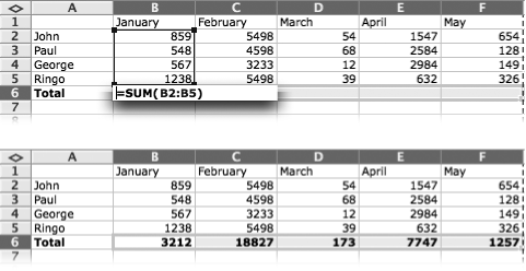
Down, Up. Fills the selected block of cells with whatever’s in the top or bottom cell of the selected block. You might use one of these commands when setting up a series of formulas in a column that adds a row of cells.
Right, Left. Fills the selected range of cells with whatever’s in the leftmost or rightmost cell. For example, you’d use this feature when you need to put the same total calculation at the bottom of 23 different columns.
Across Worksheets. Fills the cells in other sheets in the same workbook with the contents of the selected cells. For example, suppose you want to set up worksheets that track inventory and pricing over different months in different locations, and you want to use a different worksheet for each location. You can fill in all of the general column and row headings (such as part numbers and months) across worksheets with this command.
To make this work, start by selecting the cells whose contents you wish to copy. Then select the sheets you want to fill by Shift-clicking a group of sheet tabs or ⌘-clicking non-contiguous sheet tabs at the bottom of the window. (If you can’t see all the tabs easily, drag the slider between the tabs and the horizontal scroll bar. When you drag it to the right, the scroll bar shrinks, leaving more room for the tabs.)
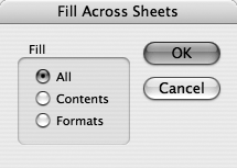
Choose Edit → Fill → Across Sheets. A small dialog box (see Figure 12-8) asks whether you want to copy data, formats, or both across the selected worksheets. Make your choice by clicking one of the radio buttons, and then click OK.
Series. Fills the selected cells with a series of increasing or decreasing values based on the contents of the topmost cell (if the selected cells are in a column) or the leftmost cell (if the cells are in a row).
For example, suppose you’re about to type in the daily statistics for the number of dot-com startups that went out of business during the first two weeks of 2008. Instead of having to type 14 dates into a row of cells, you outsource this task to Excel.
Enter 1/1/2008 in a cell. Then highlight that cell and the next 13 cells to its right. Now choose Edit → Fill → Series. The Series window appears, where you can specify how the fill takes place. You could make the cell labels increase by months, years, every other day, or whatever. Click OK; Excel fills the cells with the date series 1/1/2008, 1/2/2008, 1/3/2008, and so on.
Tip
The above example reflects the way Americans write dates, of course. If you use a different system for writing dates (perhaps you live in Europe or Australia), and you’ve used the Mac’s International preference pane (choose
 → System Preferences) to specify that you like January 14, 2008 written 14/1/2008, the next time you launch Excel it automatically formats dates the way you like them.
The other options in this dialog box include Linear (adds the amount in the Step field to each successive cell’s number), Growth (multiplies by the number in the Step field), and AutoFill (relies on the lists described in the next section).
Justify. Spreads the text in a single cell across several cells. You’d use this function to create a heading that spans the columns beneath it. If the cells are in a row, this command spreads the text in the leftmost cell across the selected row of cells. If the cells are in a column, it breaks up the text so that one word goes into each cell.
Note
At this writing, the Justify command doesn’t work in the current version of Excel (version 12.0). Until Microsoft fixes it, you can achieve the same effect by selecting the group of cells, choosing Format → Cells → Alignment, and choosing Center Across Selection from the Horizontal pop-up menu.
You don’t have to use the Edit → Fill submenu to harness the power of Excel’s AutoFill feature. As a timesaving gesture, Microsoft also gives you the fill handle (see Figure 12-9), a small square in the lower right of a selection rectangle. It lets you fill adjacent cells with data, exactly like the Fill commands—but without a trip to a menu and a dialog box.
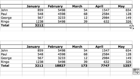
Figure 12-9. To use the fill handle, select the cell containing the formula or values you want to replicate and drag the tiny fill handle at the lower-right corner of the selection across the cells you want to fill. When you release your mouse, Excel fills the cells and displays the smart button, giving you the option to fill with or without formatting, or with formatting only.
To use it, select the cells containing the data you want to duplicate or extend, then drag the tiny fill handle across the cells where you want the data to be, as shown in Figure 12-9. Excel then fills the cells, just as though you’d used the Fill Down, Right, Up, or Left command. (To fill a series, Control-click the handle and choose an option from the shortcut menu.)
Tip
Excel can perform some dramatic and complex fill operations for you if you highlight more than one cell before dragging the fill handle. Suppose, for example, that you want to create a list of every third house number on your street. Enter 201 Elm St. in the first cell, then 204 Elm St. in the next one down. Highlight both of them, and then drag the fill handle at the lower-right corner of the second cell downward.
Excel cleverly fills the previously empty cells with 207 Elm St., 210 Elm St., 213 Elm St., and so on.
What’s more, the fill handle can do smart filling that you won’t find on the Edit → Fill submenu. For example, if you type January into a cell and then drag the fill handle across the next bunch of cells, Excel fills them with February, March, and so on; ditto for days of the week. Drag beyond December or Saturday, and Excel starts at the series over again. In fact, if you type January, March, drag through both cells to select them, and then drag the fill handle across subsequent cells, Excel fills them in with May, July, and so on. How cool is that?
What’s more, you can teach Excel about any other sequential lists you regularly use in your line of work (NY Office, Cleveland Office, San Diego Office, and so on). Just choose Excel → Preferences → Custom Lists panel; click Add and then type the series of items in order, each on its own line. Click OK; the AutoFill list is now ready to use.
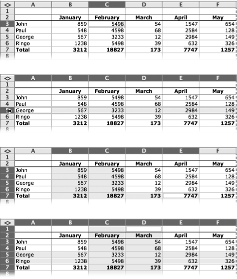
Selecting a single cell in Excel is easy. Just click the cell to select it. Often, though, you’ll want to select more than one cell—in readiness for copying and pasting, making a chart, applying boldface, or using the Fill command, for example. Figure 12-10 depicts all you need to know for your selection needs.
Select a single cell. To select a single cell, click it or enter its address in the Name box (which is shown in Figure 12-1) or press F5.
Select a block of cells. To select a rectangle of cells, just drag diagonally across them. You highlight all of the cells within the boundaries of the imaginary rectangle you’re drawing. (Or click the cell in one corner of the block and then Shift-click the cell diagonally opposite.)
Select a noncontiguous group of cells. To select cells that aren’t touching, ⌘-click (to add individual independent cells to the selection) or ⌘-drag across cells (to add a block of them to the selection). Repeat as many times as you like; Excel is perfectly happy to highlight random cells, or blocks of cells, in various corners of the spreadsheet simultaneously.
Select a row or column. Click a row or column heading (the gray label of the row or column).
Select several rows or columns. To select more than one row or column, drag through the gray row numbers or column letters. (You can also click the first one, then Shift-click the last one. Excel highlights everything in between.)
Figure 12-10. You can highlight spreadsheet cells, rows, and columns in various combinations. You can copy using rectangular-shaped selections, but you can apply cell formatting changes to any group of selected cells. Top: Click a cell (or arrow-key your way into it) to highlight just one cell. Second from top: Click a row number or column letter (row 5, in this case) to highlight an entire row or column. Third from top: Drag to highlight a rectangular block of cells; add individual additional cells to the selection by ⌘-clicking. Bottom: ⌘-click row headings and column headings to highlight intersecting rows and columns.
Select noncontiguous rows or columns. To select two or more rows or columns that aren’t touching, ⌘-click, or ⌘-drag through, the corresponding gray row numbers. You can even combine these techniques—highlight first rows, then columns, and voilà! Intersecting swaths of highlighting.
Select all cells. Press ⌘-A to select every cell on the sheet—or just click the gray, far upper-left rectangle with the diamond in it.
Once you’ve selected some cells, you can move their contents around in various ways—a handy fact, since few people type everything in exactly the right place the first time. Excel only lets you copy groups of cells that are basically rectangular in shape or that share the same rows and multiple columns or the same columns in multiple rows. Figure 12-11 shows some acceptable and unacceptable selections for copying.
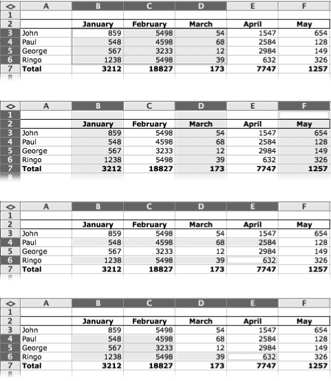
Figure 12-11. Thou shalt copy multiple cells by selecting a rectangular group of cells, an entire row or column, multiple rows or columns, or matching groups of cells in various rows or columns. The three upper examples are acceptable, the bottom one is not. If you try to copy a group of cells and don’t follow these selection rules, Excel informs you of your error: “That command cannot be used on multiple selections.”
Just as in any other Mac program, you can use the Edit menu commands—Cut (⌘-X), Copy (⌘-C), and Paste (⌘-V)—to move cell contents around the spreadsheet—or to a different sheet or workbook altogether. When you paste a group of cells, you can either select the same number of cells at your destination, or select just one cell—which becomes the upper left cell of the pasted group.
But unlike other Mac programs, Excel doesn’t appear to cut your selection immediately. Instead, the cut area sprouts a dotted, moving border, but otherwise remains unaffected. It isn’t until you select a destination cell or cells and select Edit → Paste that the cut takes place (and the shimmering stops).
Tip
Press the Esc key to make the animated dotted lines stop moving, without otherwise affecting your copy or cut operation. One more piece of advice: Check the status bar at the bottom of the window to find out what Excel thinks is happening (“Select destination and press ENTER or choose Paste,” for example).
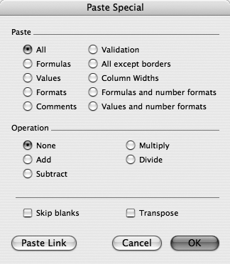
The Edit → Paste Special command summons a dialog box inquiring about how and what to paste. For example, you might decide to paste the formulas contained in the material you copied so that they continue to do automatic math—or only the values (the results of the calculations as they appear in the copied material).
Tip
This dialog box also contains the mighty Transpose checkbox, a tiny option that can save your bacon. It lets you swap rows-for-columns in the act of pasting, so that data you input in columns winds up in rows, and vice versa. This kind of topsy-turvy spreadsheet modification can be a great help if you want to swap the orientation of your entire spreadsheet, or copy a group of cells between spreadsheets which have juxtaposed rows and columns.
Excel also lets you grab a selected range of cells and drag the contents to a new location. To do this, select the cells you want to move, then point to the thick border on the edge of the selection, so that the cursor changes into a little hand that grabs the cells. You can now drag the selected cells to another spot on the spreadsheet. When you release the mouse button, Excel moves the data to the new location, exactly as though you’d used Cut and Paste.
You can modify how dragging and dropping items and Excel works by holding down these modifier keys:
Option. If you hold down the Option key, Excel copies the contents to the new location, leaving the originals in place.
Shift. Normally, if you drag cells into a spreadsheet area that you’ve already filled in, Excel asks if you’re sure you want to wipe out the cell contents already in residence. If you Shift-drag cells, however, Excel creates enough new cells to make room for the dragged contents, shoving aside (or down) the cell contents current occupants in order to make room.
Option and Shift. Holding down both the Option and Shift keys as you drag copies the data and inserts new cells for it.
Control. Control-dragging yields a menu of 11 options when you drop the cells. This menu lets you choose whether you want to move the cells, copy them, copy just the values or formulas, create a link or hyperlink, or shift cells around. It even lets you cancel the drag.
Suppose you’ve just completed your spreadsheet cataloging the rainfall patterns of the Pacific Northwest, county by county, and then it hits you: You forgot Humboldt County in California. Besides the question of how you could possibly forget Humboldt County, the larger question remains: What do you do about it in your spreadsheet? Delete the whole thing and start over?
Fortunately, Excel lets you insert blank cells, rows, or columns into existing sheets through the Insert menu. Here’s how each works.
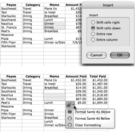
Cells. The Insert → Cells command summons the Insert dialog box. It lets you insert new, blank cells into your spreadsheet, and lets you specify what happens to the cells that are already in place—whether they get shifted right or down. See Figure 12-13.
Rows. If you choose Insert → Rows, Excel inserts a new, blank row above the active cell.
Figure 12-13. When you select cells and then choose Insert → Cells, Excel asks where you want to put the new cells (top). The two buttons at the bottom let you insert entire rows or columns. Excel then inserts the same number of cells as you’ve selected in the location selected, and moves the previous residents of those cells in the direction that you specify (bottom). In addition, the Format smart button appears, giving you three choices: format your new cells to match those above, those below, or without formatting at all.
Columns. If you choose Insert → Columns, Excel inserts a new blank column to the left of the active cell. If you’ve selected a range of cells, Excel inserts the number of columns equal to the number of columns selected in the range.
Warning
If the cells, columns, or rows that you send shifting across the spreadsheet by inserting cells already contain data, you can mangle the entire spreadsheet in short order. For example, data you entered in the debit column can suddenly end up in the credit column. Proceed with extreme caution.
Exactly as in Word, Excel has both a Find function, which helps you locate a specific spot in a big workbook, and a Replace feature that’s ideal for those moments when your company gets incorporated into a larger one, requiring its name to be changed in 34 places throughout a workbook. The routine goes like this:
Highlight the cells you want to search.
This step is crucial. By limiting the search range, you ensure that your search-and-rescue operation won’t run rampant through your spreadsheet, changing things you’d rather leave as is.
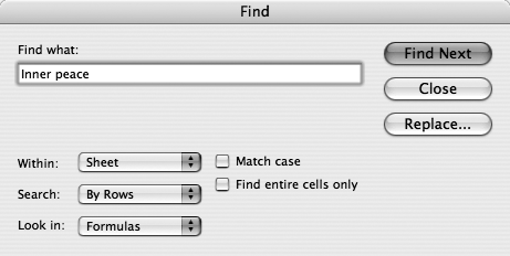
Choose Edit → Find. In the resulting dialog box, specify what you want to search for, and in which direction (see Figure 12-14).
You can use a question mark (?) as a stand-in for a single character, or an asterisk (*) to represent more than one character. In other words, typing P?ts will find cells containing “Pats,” “Pots,” and “Pits”; while typing P*ts will find cells containing “Profits,” “Prophets,” and “Poltergeists.”
The “Find entire cells only” checkbox means that Excel will consider a cell a match for your search term only if its entire contents match; a cell that says “Annual profits” isn’t considered a match for the search term “Profits.”
Figure 12-14. Using the Search pop-up menu, you can specify whether Excel searches the highlighted cells from left to right of each row (“By Rows”) or down each column (“By Columns”). Use the “Look in” pop-up menu to specify which cell components are fair game for the search: formulas, values (that is, the results of those formulas, and other data you’ve typed into the cells), or comments. Turn on “Match case” if you’re trying to find “Bill” and not “bill.”
If you intend to replace the cell contents (instead of just finding them), click Replace; type the replacement text into the “Replace with” box. Click Find Next (or press Return).
Each time you click Find Next, Excel highlights the next cell it finds that matches your search phrase. If you click Replace, you replace the text with the “Replace with” text. If you click Replace All, of course, you replace every matching occurrence in the selected cells. Use caution.
“Erase,” as any CIA operative can attest, is a relative term. In Excel, the Edit → Clear submenu lets you strip away various kinds of information without necessarily emptying the cell completely. For example:
Edit → Clear → All truly empties the selected cells, restoring them to their pristine, empty, and, unformatted condition. (Control-B does the same thing.)
Edit → Clear → Formats leaves the contents, but strips away formatting (including both text and number formatting).
Edit → Clear → Contents empties the cell, but leaves the formatting in place. If you then type new numbers into the cell, they take on whatever cell formatting you had applied (bold, blue, Currency, and so on).
Edit → Clear → Comments deletes only electronic yellow sticky notes (see Flag for Follow-Up).
None of these is the same as Edit → Delete, which actually chops cells out of your spreadsheet and makes others slide upward or leftward to fill the gap. (Excel asks you which way you want existing cells to slide.)
If you’ve never used a spreadsheet before, the concepts described in the previous pages may not make much sense until you’ve applied them in practice. This tutorial, which continues with a second lesson on Tutorial 2: Yearly Totals, can help.
Suppose that you, Web marketer extraordinaire, are preparing to write your next bestseller, The Two-Hour Workweek, and you’d like to include some facts and figures about your remarkable rise to success. So you cancel your morning hang gliding lesson and crank up Excel to get a handle on your years of part-time toil.
Create a new spreadsheet document by choosing File → New (⌘-N).
Excel fills your screen with the spreadsheet grid; the first cell, A1, is selected as the active cell, awaiting your keystrokes.
Begin by typing the title of your spreadsheet in cell A1.
Profit and Loss Statement: Time is Not Money might be a good choice. As you type, the characters appear in the cell and in the Edit box in the Formula bar.
Click outside of cell A1 to get out of the entry mode, click back on cell A1 to highlight it, and then press ⌘-B.
Excel inserts your text into cell A1. Since all the cells to the right of A1 are empty, Excel runs the contents of cell A1 right over the top of them. When you press ⌘-B, Excel formats the first cell’s text in bold, to make a more impressive title for your spreadsheet.
Press Return three times. And then press ⌘-S.
Excel moves the active cell frame down a couple of rows, selecting cell A4. Even if you haven’t entered any data yet, save the spreadsheet by pressing ⌘-S (or choosing File → Save), naming it, and then choosing a suitable destination. Now as you continue to work on your spreadsheet, periodically press ⌘-S to save your work as you go along.
Type January.
You need to track expenses over time: to track the project by calendar year, name the first column January. You could now tab to the next cell, enter February, and work your way down the spreadsheet—but there’s an easier way.
As noted earlier, Excel can create a series of months automatically for you, saving you the effort of typing February, March, and so on—you just have to start it off with the first entry or two.
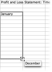
Click once outside cell A4 to get out of entry mode, and then click cell A4 again to select it. Carefully click the tiny square at the lower-right corner of the highlighted cell; drag directly downward through 11 more cells.
Pop-out yellow screen tips reveal what Excel intends to autofill into the cells you’re dragging through. When the screen tip says December, stop.
Excel enters the months and highlights the cells you dragged through. Figure 12-15 shows this step.
Now it’s time to add the year headings across the top.
Click cell B3 to select it. Type 2004. Press Tab, type 2005, and then press Enter.
You’ll use the same AutoFill mechanism to type in the names of the next four years. But just dragging the tiny square AutoFill handle on the 2004 cell wouldn’t work this time, because Excel wouldn’t know whether you want to fill every cell with “2004” or to add successive years. So, you’ve given it the first two years as a hint.
Drag through the 2004 and 2005 cells to highlight them. Carefully click the tiny square at the lower-right corner of the 2005 cell; drag directly to the right through three more cells.
Excel automatically fills in 2006, 2007, and 2008, using the data in the first two cells to establish the sequence.
If you like, you can now highlight the year row, the month column, or both, and then press ⌘-B to make them boldface (see Figure 12-16). Chapter 13 has more details on formatting your spreadsheets.
Now that the basic framework of the spreadsheet is in place, you can begin typing in actual numbers.
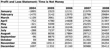
Figure 12-16. You can make the headings stand out from the data you’ll soon put in the cells by changing the font style and alignment (see Chapter 13). In this example, the row and column headings are bold, and the column headings are centered.
Click cell B4, January 2004. Enter a figure for your January income.
Your first several months of operation showed a loss since you were investing in lots of “Get Rich Quick on the Internet!” programs. You invested heavily at the beginning, and your losses in January were $1,895. Since this is a loss, enter it as a negative number, and leave off the dollar sign—just type -1895.
Press Return (or the down arrow key).
Excel moves the active cell frame to the next row down.
Type another number to represent your loss for February; press Return. Repeat steps 9 and 10 until you get to the bottom of the 2004 column.
For this experiment, the exact numbers to type don’t matter too much, but Figure 12-16 shows one suggestion. Perhaps, toward the end of that first year, you started making money instead of losing money.
Click in the January 2005 column (C4); fill in the numbers for each month, pressing Return after each entry. Repeat with the other years.
Remember, this is a success story, so type ever-increasing numbers in your columns, because once you started making money, it was an ever-upward trend. But then your income kind of leveled off toward the end of 2007 as you cut back your work week to two hours.
When you’ve successfully filled your spreadsheet with data, save your work one more time. You’ll return to it later in this chapter—after you’ve read about what Excel can do with all of these numbers.