Another way you can make your data easier to interpret is to change the appearance of your data based on the value in a cell. This kind of formatting is called conditional formatting because the data must meet certain conditions to have a format applied to it. For example, if you use a worksheet to track your customers’ credit lines, you could have a customer’s outstanding balance appear in red if they are within 10 percent of their credit limit.
Excel 2007 improves upon the conditional formatting capabilities of previous versions by enabling you to create an unlimited number of conditions (you were previously limited to three), allowing more than one condition to be applied to a cell, and making it easier for you to manage your conditions.
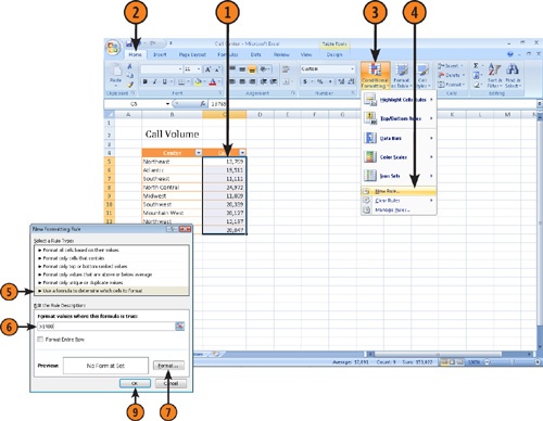
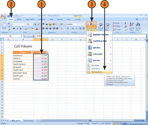
Change the Format of a Cell Based on Its Value
Select the cells you want to change.
Click the Home tab.
In the Styles group on the ribbon, click Conditional Formatting.
Click New Rule.
Click Format Only Cells That Contain.
Click the Comparison Phrase down arrow.
Click the comparison phrase you want.
Type the constant values or formulas you want evaluated.
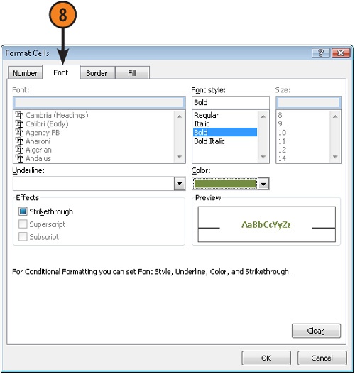
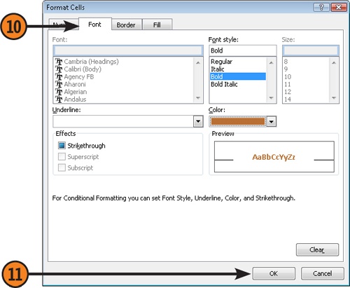
Click Format.
Specify the formatting you want and click OK.
Click OK.
Caution
The layout of the Edit the Rule Description pane changes to reflect the Rule Type you’ve chosen. Don’t be surprised if you see a different number of fields than the graphics show.
Change the Format of a Cell Based on the Results of a Formula
Select the cells you want to change.
Click the Home tab.
In the Styles group on the ribbon, click Conditional Formatting.
Click New Rule.
Click Use a formula to determine which cells to format.
Type the formula you want evaluated.
Click Format.
Specify the formatting you want and click OK.
Click OK.
Try This!
In a blank worksheet, click cell A1, click the Home tab, click the Conditional Formatting button, and then click New Rule. Define a condition that applies when a Cell Value Is Between 400 and 1000. Apply bold formatting to the cells. Click OK. Define a second condition that applies when a Cell Value Is Less Than 400. Apply italic formatting to the cells. Click OK. Type 450 in cell A1 and press Enter. The cell’s contents will be displayed in bold type. Click cell A1, type 350, and press Enter. The cell’s contents will now be displayed in italics.
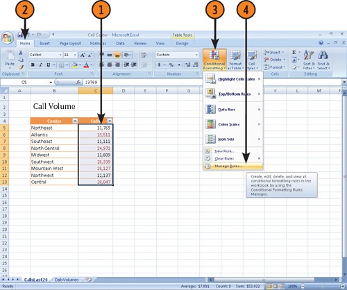
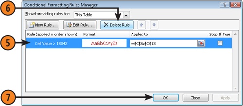
Edit a Conditional Formatting Rule
Select the cells that contain the rule you want to edit.
Click the Home tab.
In the Styles group, click Conditional Formatting.
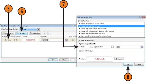
Click Manage Rules.
Click the rule you want to change.
Click Edit Rule.
Use the controls to make your changes.
Click OK twice to save your changes.
Delete a Conditional Formatting Rule
Select the cells that contain the rule you want to edit.
Click the Home tab.
In the Styles group, click Conditional Formatting.


 In the Styles group on the ribbon, click Conditional Formatting.