In this chapter, you will:
Learn to approach workbook formatting methodically
Set defaults for new workbooks
Learn about the benefits of themes and cell styles
Discover the advantages of Excel tables
Explore page layout and header and footer options
Do you think of your Microsoft Excel files as documents? If not, you might be selling them short. Text-based documents—such as reports that require complex formatting with text, tables, and graphics—surely belong in Word. But when you share an Excel file containing worksheet data, charts, or maybe even PivotTable reports, you are absolutely sharing a document.
So, in the first of this book’s chapters on Excel 2010 and Excel for Mac 2011, we’re looking at formatting documents. From cells, rows, and columns to worksheets and workbooks, this chapter is all about letting your Excel files shine like the documents they are. Of course, because much of your Excel document content is dynamic, much of the formatting is as well. That is, there’s more to formatting your Excel worksheet content than a well-chosen font or color. Formatting Excel documents effectively can mean making your data do more for you.
As for what’s new and improved for formatting worksheets in Excel, users of Excel 2010 who are already familiar with Excel 2007 won’t see many differences, but you do get some welcome additional flexibility. The most exciting improvements in this area are in conditional formatting. The new and improved list is a bit longer for Excel 2011 users, with many formatting capabilities that are now quite similar to those in Excel 2010.
Whether you’re a Windows or Mac user, the core concepts of Excel are unchanged. It is still the best home for your data, lord of the number crunchers, and master of logic. When it comes to formatting worksheet content, in a nutshell, this chapter covers how your worksheets can be better looking and more dynamic than you might imagine.
If the idea of formatting worksheet content isn’t exhilarating, and you’re tempted to skip ahead to the sexier topics of sparklines, charts, or PivotTables, give it a minute. Some of the tools that you’re likely to use most often are addressed in this chapter: Excel tables, themes, cell styles, and page layout. The more you know about these tools, the faster you’ll be able to apply them in your workbooks. And that means you’ll have more time to experiment with those racier topics.
Note
See Also To learn about conditional formatting, including what’s new for these features on both platforms, see Chapter 19, where you can also learn about the brilliant new sparklines feature. For help working with Excel charts, see Chapter 20. And to learn about working with PivotTables, see Chapter 21.
For Mac Users
The big stories for worksheet formatting in Excel 2011 are tables and conditional formatting. But there are other key new and improved features as well, including cell styles. Additionally, a great many formatting options previously available across the menus and formatting palette are nicely exposed on the Home and Layout tabs, giving you easy access to some handy tools that you might have missed in the past.
It’s also important to note that, because themes are now extended to your worksheets, your formatting options have greatly increased. This also means that a 32-bit color palette and the Apple Color Picker for custom colors are now available for all features that support color. The 40-color limitation has been removed, and now your color choices are now almost endless.
Check out a few of the key changes for formatting worksheets:
Excel tables are the evolution of the List feature from previous versions, and quite an impressive evolution it is. When you format a range as a table, you get additional functionality, much of which is on the Tables tab, shown in Figure 17-1.
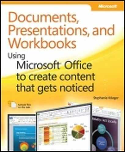
Conditional formatting (as you see in Figure 17-2) is tremendously improved, both with dramatic new data visualization options and the ability to manage formatting rules throughout the workbook from a single dialog box.
Cell styles, shown in Figure 17-3, are a type of Quick Style that you can customize and even copy between workbooks.

Note
Along with many new features for the content in your workbooks, you also get better document management for the workbooks themselves. It’s likely that you’ll never again see that dreaded dialog box telling you that Excel is unable to open a file that is damaged or that contains unreadable content. The new Open & Repair feature in Excel 2011 will offer to repair the workbook instead of refusing to open it.
Note
See Also Learn about formatting Excel tables, using themes in Excel, and using cell styles later in this chapter. For information about the data-management capabilities of Excel tables, see Chapter 18. And to learn about conditional formatting, see Chapter 19.
Unlike Word, where document formatting is about a robust, professional finished product that gets your content noticed, Excel has always been about function rather than form. However, you don’t have to sacrifice one for the other.
Much of the available formatting in Excel is tied to the functionality, such as tables or conditional formatting. So, when you make your documents look better, you also have the opportunity to make them perform better.
For this reason, when you work in Excel, it’s essential to think about what you need the content of your worksheets to do while you’re addressing how you want them to look. Consider the following examples.
When formatting a range of cells, instead of just applying borders, shading, or font color individually, think about the reasons you’re formatting that range as a unit. Can you format that range as a table instead, and then take advantage of the additional functionality that Excel tables offer?
If your workbook includes several sheets, do you format related ranges or related sheets consistently? When data from one sheet to the next is related, applying related formatting can do more than help your workbook look professional. You can also use consistent formatting across ranges or worksheets to make the logic of your workbook more intuitive for recipients.
Just as when you’re working in Word, avoid getting carried away with formatting in Excel. Remember, the purpose of formatting is to help make your information shine through.
In Excel, this concept goes a step further because Excel documents are often dynamic work products that need to continue to change after you’ve delivered them. Overly formatted worksheets can be difficult to read and make it harder to understand the logic in your data. Always consider the workbook as a whole and choose consistent formatting that, where appropriate, can add functionality to your worksheets.
Note
See Also For some best practices to consider when you’re planning any Microsoft Office documents, including those you create in Excel, see Chapter 4.
Formatting worksheet content has traditionally been a source of stress for many Excel users, because it’s quite inflexible compared to formatting documents in Word or even in PowerPoint. If you combine the formatting capabilities in Excel with a methodical approach to worksheet formatting, however, that stress can be a thing of the past.
Taking a methodical approach in this case means to remember that, regardless of what part of a workbook you’re using, the entire workbook is a single unit. The workbook is composed of sheets, which are composed of rows and columns, which are in turn composed of cells.
Why state what seems to be so obvious? Because, if you’re like most Excel users, you don’t usually think about this, and it can show in your formatting. More importantly, it can also show in your frustration when you need to edit workbooks. To work more effectively and with less stress when formatting content in Excel, keep some of the same concepts in mind that you would when formatting Word documents.
For example, to do the least work possible, start by formatting the largest possible portions of the document (workbook) first.
Apply whatever you can to the entire workbook (such as applying a theme and setting workbook defaults).
Note
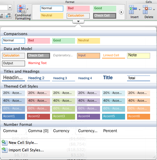
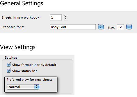
One of the easiest things you can do to save time when formatting workbooks is to set your formatting defaults for new workbooks. To do this, in Excel 2010, click the File tab and then click Options. On the General tab, in addition to settings that apply throughout several of the 2010 release programs, you’ll see the options in Figure 17-4 for creating new workbooks. In Excel 2011, from the Excel menu, click Preferences. New workbook options are in the General and View settings, shown in Figure 17-5.
Set formatting that applies to one or more sheets at a time (such as setting row height or applying headers and footers).
Format specific ranges or tables.
Format individual cells that require different formatting from the applicable range or table.
In addition to helping you do less work, approaching the workbook methodically also helps you stay in control of formatting. The following points may also be useful to keep in mind:
Remember that formatting applied to individual cells takes priority over the formatting of ranges, tables, or worksheets. This is similar to the way character formatting takes precedence over paragraph formatting in Word. So, for example, if you format a table and then apply unique formatting to a few cells in the table, that unique cell formatting will remain intact when you apply a new table style.
When you copy or move cells, rows, or columns, the formatting travels along by default. Use Paste Options, addressed in the upcoming Insider Tip sidebar, to get the result you need and avoid having to fix unwanted formatting later.
As you can see from the preceding recommendations, working methodically in Excel is very similar to working methodically in Word, or for that matter, in any software program. That’s because, though much of what goes into creating effective documents is about knowing the features of the program and how to use them, the other key ingredient has nothing to do with software. Creating effective Microsoft Office documents requires paying attention to what’s happening them so that you can stay in control of their content. It requires a bit of planning and organization so that you can keep things as simple as possible, and focus on the product rather than the process.
Note
The simplest tools can sometimes be the most useful when you’re looking for ways to format documents effectively. For example, use simple keyboard shortcuts to get exactly what you need with less work. Two that come in handy for Excel worksheet formatting are Alt+Enter (Control+Option+Enter in Excel 2011), which wraps text to a new line within the same cell, and Ctrl+Enter, which fills all cells in a selected range with the same content. To use Ctrl+Enter, select the range to fill, type the content you need as if you were working in a single cell, and then press Ctrl+Enter (instead of Enter alone) to fill all cells in the selected range.
Note
See Also For complete coverage of theme basics, including the components of themes (fonts, colors, and effects), how to apply them, and how to save a custom theme, see Chapter 5.
When formatting your worksheets, remember to apply theme-ready formatting by selecting from options specified as applicable to themes. That is, select fonts from the Theme Fonts options at the top of font drop-down lists and select colors from the Theme Colors portion of the color palette, both shown in Figure 17-6.
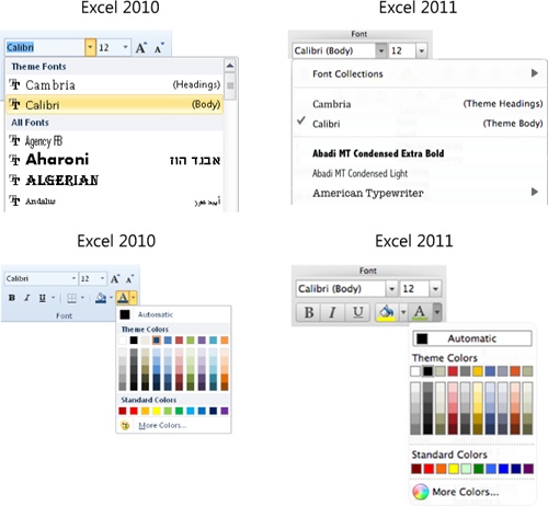
Remember, if you select a font or specify a color that’s used in the active theme but don’t select it from the theme options, your formatting won’t be theme-ready—meaning that it won’t update to take on new formatting when you change the active theme.
Note
When you need to use a theme that was created on another computer, remember that you can also copy a custom theme from any document. To access this option in Excel 2010, on the Page Layout tab, click Themes and then click Browse For Themes. In Excel 2011, on the Home tab, click Themes and then click Browse Themes. Because you have the same themes available in Word, Excel, and PowerPoint, you can copy the theme from a theme-ready document created in any of these programs.
New workbooks are set to take on the active theme’s body font by default. As shown earlier, to access defaults for new workbooks, in Excel 2010, click the File tab, click Options and then click General. In Excel 2011, from the Excel menu, click Preferences and then click General. You’ll find default settings including font, font size, number of sheets, and for Excel 2010, default view. The default view for Excel 2011 is located in the View settings.
Note
In Excel 2010, if you hover your mouse pointer over the list of available options in the Theme Fonts gallery, Live Preview shows a small change in the appearance of your workbook even if the workbook is blank. That’s because row and column headings automatically take on the body font of the active theme.
It’s worth noting here that theme effects apply to Excel charts much as they do to other graphics, such as SmartArt diagrams. To use theme effects with charts, first apply a chart style that uses graphic effects. Then, you’ll see theme effects change when you apply a different theme or, in Excel 2010, when you preview or apply different theme effects.
In Excel 2010, when you hover your mouse pointer over the various options in the theme effects galleries, you’ll see different variations on the chart style for each set of theme effects.
In Excel 2011, even though you don’t have a separate theme effects gallery, you can still make use theme effects to format charts and other Office Art objects. Just start with a theme that uses your desired effects and then select different theme color and theme font sets as needed to create your custom look.
To keep worksheet formatting streamlined, consider using styles in Excel in much the same way you do in Word. Between cell styles and table styles, you can save time, keep your formatting more consistent, and create theme-ready workbooks more easily. In the next two sections of this chapter, you’ll learn about cell and table styles and how they interact with themes.
Cell styles are the evolution of the extremely limited Styles feature that you might know from earlier versions of Excel. The current cell styles feature, first introduced in Excel 2007, is part of the Quick Styles functionality that you see for many features across Office 2010 and Office for Mac 2011.
Note
Excel 2011 still has the Style command under the Format menu, but it doesn’t provide access to the full range of available styles. This command now lets you modify only the Normal style, which you can also accomplish from the Cell Styles gallery, discussed next.
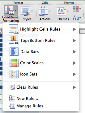
Notice that the Cell Styles gallery, shown in Figure 17-7, includes a few categories of built-in styles.

Figure 17-7. Use the Cell Styles gallery, shown here in Excel 2010, to apply several formats at the same time.
Note the following when using built-in cell styles from this gallery:
Styles in the Good, Bad, And Neutral (Comparisons in Excel 2011) and Data And Model categories are not entirely theme-ready, meaning that although they use the active theme body font, they don’t use theme-ready colors. This is intentional so that a certain color can take on a specific meaning (such as green for good, or red for bad) that will apply regardless of your applied theme.
In the same categories mentioned in the preceding bullet, style names might give you the impression that they have added functionality beyond formatting. They don’t. These style names are just suggestions for how you might use cell styles to indicate certain types of results. However, in those cases, it’s better to use conditional formatting instead so that the formatting will change, based on criteria, to always reflect the intended sentiment.
Though the styles in the Titles And Headings category look very much like some built-in Word paragraph styles, remember that you are still working in Excel. The borders used on some of these styles, for example, are cell borders. So, if your text will exceed the cell in which you type it, be sure to apply the appropriate style to all cells across which the text stretches if you want the border to appear throughout the heading.
Even though there is a category called Themed Cell Styles, the styles under the Titles And Headings category are also entirely theme-ready.
Number Format styles are carry-overs from the old Styles feature, and they apply only number formatting by default. Using these styles instead of using a number format directly from the Format Cells dialog box is beneficial when you need to update the formatting. After you apply a style to cells, whenever you modify the style, the formatting of cells that use that style updates automatically.
The Number Format styles can also be applied using the associated buttons on the Home tab in the Number group. For example, if you click the Percent format, you’re actually applying the Percent style.
Note
As just noted, the Currency, Percentage, and Comma buttons in the Number group will apply the number format defined in the associated style. There’s no rule that says you must use these buttons for those number formats—they’ll apply whatever formatting you defined in the associated style.
You can create your own styles, modify built-in styles, duplicate built-in styles to create your own variations, or delete any unwanted styles. Any of these modifications are made for the active workbook only. Of course, you can save any workbook as a template to use for creating future workbooks.
Note
See Also For help creating Excel templates, see Chapter 22.
Why Does One Cell Style Sit on Top of Another?
A cell can contain only one cell style at a time, but it’s common for cells to appear as though the first style remains when the new style is applied. This is because each cell style can include any of six unique sets of attributes (Number, Alignment, Font, Border, Fill, and Protection), as you see in Figure 17-8. Notice that these categories correspond to the six tabs of the Format Cells dialog box.
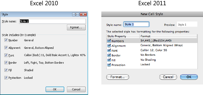
Some styles have settings for all six of these categories, but many of the built-in styles use only certain categories (such as the Number Format styles). When you apply a new style that doesn’t use all categories to a selection of cells, formatting from unused categories remains unchanged, regardless of whether that formatting was part of a style. However, the new style becomes the recognized style for those selected cells. By “recognized” style, I mean that if you edit the most recently applied style, the cell appearance will change, whereas modifying a style that was applied earlier will not affect cells that still contain some attributes of that style but have since had a new style applied.
This behavior makes cell styles far more practical, because you might often want to change font, fill, or alignment formatting, for example, where you don’t want to change number format or borders. However, to keep your custom cell styles intuitive for all users and to avoid confusion, you might want to develop a naming convention that indicates which categories are used.
You can create cell styles based on the formatting in a selected cell (referred to as By Example) or based on an existing cell style. To create a style by example, select the cell to use as the basis for your style before proceeding with the following steps:
On the Home tab, expand the Cell Styles gallery and then either click New Cell Style (to create a style by example) or right-click an existing style and then click Duplicate.
Select the categories you want to include in your new style. When you create a style by example, all categories are selected by default. When you duplicate a style, the selected categories will match the duplicated style.
Click the Format button to access the Format Cells dialog box. Remember that the tabs in this dialog box correspond to the cell style categories. Select each tab you need, customize desired attributes, and then click OK.
Confirm that the settings you customized in the Format Cells dialog box appear by each category name, as applicable, in the Style dialog box. Name your style and then click OK. Your new style will appear in the Cell Style gallery under a Custom category heading.
To modify a cell style, right-click the style name in the gallery and then click Modify to access the Style dialog box. Notice that you can also delete styles from the shortcut menu that appears when you right-click. You can delete any cell style other than Normal. However, note that built-in styles are deleted only from the active workbook. (Also note that, if you delete a style, relevant formatting is removed from any cells in the workbook to which that style was applied.)
To copy all cell styles from another workbook, start by opening the workbook containing the style definitions you want. Then do the following:
This action imports your own custom styles from the selected workbook and gives you the option to update the formatting of styles that exist in both workbooks (including built-in styles).
When you format a range as a table, you get the benefit of table styles, enabling you to apply several formatting attributes at once. But that’s just the beginning of what you can do with Excel tables. Following are some of their additional formatting-related capabilities.
The table automatically expands when you add adjacent data in rows or columns, so the newly added data is formatted to match your table without any extra work.
If you discover your formatting for a specific column isn’t being carried over to new rows, it’s usually due to mixed formatting in that column. To fix this issue, select all of the cells in the column, including those in your rows, and reapply the format.
Drag the sizing handle, shown at left, which appears on the bottom-right corner of all tables, to resize the table range. You can drag left, right, up, or down.
Simply drag selected table rows or columns to reorder them. When you select rows or columns and then hover your mouse pointer over any edge of that selection, the cursor changes to a multipointed arrow in Excel 2010 and a hand in Excel 2011. When you see this cursor, just drag the selected rows or columns. A gray bar appears, indicating where the selection will fall when you release the pointer.
If you drag just a few cells from a row or column, Excel will assume that you want to replace the destination cells, as it does when you drag cells on a worksheet outside of a table, and will prompt you accordingly. You can drag to reorder only complete rows or columns in a table.
Just right-click for the options to insert, delete, or select table rows and columns.
Note
See Also Beyond the formatting capabilities of tables are powerful data-management tools, which enable you, for example, to quickly create calculated columns, use structured references in formulas, and export table data for other uses such as a Microsoft Visio 2010 PivotDiagram. For information about working with the data-management capabilities of tables, see Chapter 18.
To format a range of data as a table, first click in or select the range to use as your table. Your range does not need to contain data prior to you creating your table. Notice that when you start with an existing contiguous data range, you don’t have to select the range first—just click somewhere in the range, and Excel will recognize it automatically. Then, do the following.
On the Home tab, click Format As Table and then click the table style that you want to apply. Or, on the Insert tab, click Table.
In the Format As Table dialog box, Excel will confirm what it believes to be the correct range for your table. If it’s not correct, you can simply drag to select the correct range without closing the dialog box. (The dialog box has a range selection icon, but you don’t need to use it to access the worksheet.)
With the Format As Table dialog box still open, if your selected range includes table headers, check the box labeled My Table Has Headers. If not, leave that box blank, and a header row will be added. Click OK to format the table.
On the Tables tab, in the Tables Styles group, click your desired table style in the gallery. Or, on the Tables tab, click New to insert a table using the default table style.
The contiguous data range will be used for your table. If this isn’t the correct range, drag the sizing handle in the bottom-right corner of the table to resize the table range.
Note
If Excel views the first row as field names—for example, if it has a text entry in each cell—it will be used as your header row. Otherwise, a new header row will be added. To select the option to include or exclude header rows when you create the table, on the Tables tab, in the Table Options group, click the arrow beside the New command.
If you create the table from any option other than the Table Styles gallery in either Excel 2010 or Excel 2011, the default table style for the active workbook will be applied to the new table.
If you want to apply a different style after creating the table, you can do this in Excel 2010 either from the Home tab, in the Format As Table gallery, or from the Table Tools Design tab, in the Table Styles gallery. In Excel 2011, on the Tables tab, use the Table Styles gallery.
In addition to the built-in table styles that you see in the gallery, you can further customize table formatting, such as adding or removing formatting from the header row or first/last column. In Excel 2010, these options are on the Table Tools Design tab in the Table Style Options group. In Excel 2011, they’re on the Tables tab in the Table Options group. Notice that, when you check options such as Banded Rows or Banded Columns, the previews in the Table Style gallery update to reflect the change. This is because several table styles include attributes for the various Table Style options that appear only in the previews when those options are in use.
You can’t modify built-in table styles, but you can duplicate them to create your own table styles based on them. To create your own custom table styles:
In Excel 2010, on the Home tab, click Format As Table. (Or, on the Table Tools Design tab, click the More button in the bottom-right corner of the Table Styles gallery to expand the gallery.)
In Excel 2011, on the Tables tab, hover your mouse pointer on the Table Styles gallery. Then click the arrow that appears along the bottom of the Styles gallery to expand it.
Either click New Table Style or right-click an existing style and then click Duplicate.
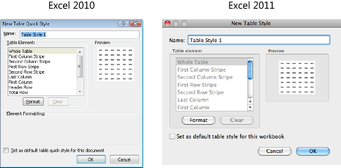
In the New Table Quick Style dialog box (New Table Style dialog box in Excel 2011), shown in Figure 17-9, select the table element to customize and then click Format. The Format Cells dialog box will open with Font, Border, and Fill options available. Set the options you want to format for the selected table element and then click OK. Repeat this action for each part of the table that you want to customize.
Figure 17-9. The New Table Quick Style dialog box for Excel 2010 and the New Table Style dialog box for Excel 2011.
In Excel 2010, once you’ve added formatting for an element, you can see a description of the element formatting below the Table Element list. For both versions, notice that you can undo any formatting applied to an individual element. Once you’ve customized a table element, the Clear option becomes available for that element.
If you want to use the new table style as the default for all tables in the active workbook, check the option Set As Default Table Quick Style For This Document (in Excel 2011, this option is named Set As Default Table Style For This Workbook.) Then, click OK to create your new style.
The style will appear under the Custom heading at the top of the Table Style gallery. In Excel 2010, it will also appear in the same location in the Format As Table gallery.
Note
You can set any table style as the document default at any time. To do this, right-click the style in the Table Styles gallery and then click Set As Default. In Excel 2010, this option is also available from the Format As Table gallery.
To modify a custom style, right-click the style and then click Modify. You can also delete a custom style from the shortcut options provided when you right-click. Built-in table styles can’t be deleted.
The Page Layout tab (Layout tab in Excel 2011), shown in Figure 17-10, is nicely organized to display most functionality you need for organized and effective worksheet formatting.
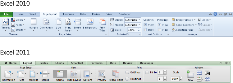
Though, as advanced users, you’re most likely already familiar with the options on this tab, note a few particular items, as follows.
Note
Depending upon your screen width, command names may not be visible for all options on the Ribbon. This is true in both Office 2010 and Office 2011, although how command names are collapsed works a bit different on each platform. Regardless, if you don’t see a command name, hover your mouse pointer on the visible command for a ScreenTip that provides more information.
For example, on the Excel 2011 Layout tab shown in Figure 17-10, some commands referred to in the list that follows may be collapsed under a group command or may be visible without command name labels.
The Page Setup group is arranged much like the Page Setup group on the same tab in Word, with Margins, Orientation, Paper Size, and even Breaks.
In Excel 2010, notice the drop-down lists for the Width and Height settings in the Scale To Fit group. Clicking the More Pages option at the bottom of either list opens the Page Setup dialog box to the Page tab, just as though you clicked the dialog launcher in the Scale To Fit group. In Excel 2011, these options are in the Print group and are named Fit To <Number Of> Page(s) Wide and Fit To <Number Of> Page(s) Tall.
One of my favorite features on these tabs is the ability to show, hide, or even print gridlines and headings. It’s so common to forget that you have these options, but easier to remember now with them clearly visible on the Ribbon. In Excel 2010, these options are in the Sheet Options group. In Excel 2011, the options to show or hide gridlines and headings are in the View group (these are collapsed under an Options command in Figure 17-10, as explained in the note that precedes this list). The options for printing them are in the Print group.
In Excel 2010, when you have graphic objects on your worksheets, note the Selection Pane option in the Arrange group. The Selection And Visibility pane—which is also available in PowerPoint 2010 and Word 2010, but is not available in Office 2011—shows every graphic (such as pictures or drawing objects) on the active sheet. It gives you easy access to select each graphic or even to choose to hide certain ones, such as if you want to print a worksheet without displaying only specific graphics.
Caution
If you use the Selection And Visibility pane in Excel 2010 to hide objects on a sheet and then open that workbook in Excel 2011, objects remain hidden. You can either open the file again in Excel 2010 to reveal hidden objects or, in Excel 2011, use Microsoft Visual Basic for Applications (VBA) to do this quickly.
If you’re already familiar with VBA, you can use the statement
?ActiveSheet.Shapes.Countin the Immediate window to determine whether objects are hidden on the sheet. Note that this count will include all graphic objects—that is, charts as well as objects like shapes and pictures. You can then either use the Immediate window to set applicable shapes to be visible, such asActiveSheet.Shapes(1).Visible=Trueor, if there are several, write a simple macro using a loop to cycle through all shapes on the sheet.If you’re not already familiar with VBA basics and would like to know how to use VBA to accomplish timesaving, troubleshooting tasks such as these, see Chapter 23.
Note
See Also If you use the Selection Pane in any applicable Office 2010 program to hide graphics, be sure to check for hidden graphics before sharing the workbook. You can do this easily using the Document Inspector, introduced in Chapter 3.
Note that this pane won’t recognize individual drawing objects created directly in Excel charts.
Unlike in Word, the Background feature in Excel is for on-screen backgrounds only and can’t be printed. To print a watermark image on a worksheet, insert a picture into the header or footer that exceeds the height of the header or footer by the amount of the page that you want to watermark. Pictures that exceed the header or footer height automatically fall behind the page.
In Excel 2010, once you insert a picture into the header or footer, the Format Picture option on the Header & Footer Tools Design tab becomes available, where you can set the image color to Washout.
In Excel 2011, to format a picture in the header or footer, switch to Page Layout view and then double-click the picture field (&[Picture]). Then, on the pop-up toolbar, click Format Picture for available options.
When working on page layout formatting, try using Page Layout view instead of Normal view. To switch to Page Layout view, in Excel 2010, use the View tab or the view shortcuts on the Status bar. In Excel 2011, Page Layout view is on the Layout tab and on the View menu.
Just as in Word, when you can actually see the page layout, it’s much easier to edit. For example, to change margins using the rulers in Page Layout, point to any margin on the horizontal or vertical ruler and do one of the following:
In Excel 2010, your insertion point will turn into a double-backed black arrow, shown at left. When it does, simply drag to change the margins.
In Excel 2011, your insertion point will turn into a small rectangle with arrows pointing left and right, as shown at left. When it does, simply drag to change the margins.
You can change margins by as little as 1/100th of an inch at a time using this method (no additional key is required for this precise resizing in Excel), and in Excel 2010, the measurement will appear in a ScreenTip as you drag.
In Page Layout view, headers and footers are also automatically visible. In fact, in Excel 2010, if you click Header & Footer on the Insert menu, your view will be changed to Page Layout view.
Note
You can still access header and footer options in the Page Setup dialog box; however, modifying your headers and footers in Page Layout view has its advantages. For example, you don’t have to stick to left, center, and right sections when you edit the header and footer directly on the page, as explained in this section. And, of course, there is the benefit that you see what your headers and footers look like while editing on the page.
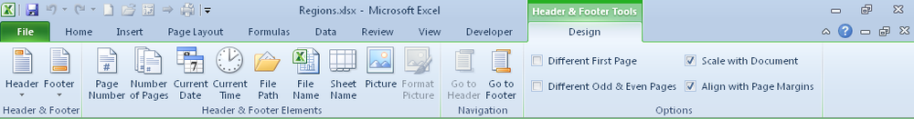
Excel 2010 offers additional benefits when you’re editing headers and footers on the page, because the Header & Footer Tools Design contextual tab (shown in Figure 17-11) that appears in this view gives you more functionality than is available in that dialog box.
To edit the header or footer, you can click into the left, center, or right areas of the header or footer directly on the sheet. You can also break the left, center, and right section barriers and create a header or footer that extends across the page. To do this, just start typing in one section. When your content exceeds the width of the active header or footer portion, the header or footer automatically becomes a single area.
Note that, although you can add and edit text in the header or footer directly on the sheet, you can’t add other elements (such as pictures) directly. In Excel 2010, objects that you can insert are displayed on the Header & Footer Tools Design tab, in the Header & Footer Elements group. In Excel 2011, these options are listed on the pop-up toolbar that appears when you click into a header or footer. (In Excel 2010, also note that even though the Font group on the Home tab is available to your content in headers and footers, many options, such as the Picture command on the Insert tab, are not.)
Note
A single header or footer is limited to a maximum of 255 characters, including formatting marks (such as spaces) and special characters.
As a final note on headers and footers for Excel 2010 users, notice the Options group on the Header & Footer Tools Design tab. It has options such as the Different First Page or Different Odd & Even Pages settings that you know from Word, along with the handy setting to scale header and footer content with the document.
Note
As in Word, the Odd Page header and footer contains the same content as the regular header and footer. However, you can enable Different Odd & Even Pages for selected sheets in Excel, whereas this option in Word can be set only for the entire document.
Also notice that the name of the active header or footer type appears at the top-left of the header area or bottom-left of the footer area so that you know whether you’re working in the regular, first page, odd page, or even page header or footers.
The many comparisons to Word formatting throughout this chapter help to make one point crystal-clear: your Excel workbooks are just as much documents as the files you create in Word. To manage your Excel documents effectively, consider not only the concepts and best practices provided in this chapter, but also the chapters in the first part of this book that apply to all of your Microsoft Office documents.
Note
See Also To help you create and share complex workbooks with confidence, see Chapters Chapter 3 and Chapter 4. And for information about sharing documents online and on the road, including capabilities and limitations for editing and sharing workbooks via Excel Web App and Excel Mobile 2010, check out Chapter 2.