
Syntax. IF(logical_test,value_if_true,value_if_false)
Definition. This function checks a logical condition and performs the first action specified after the test argument if the condition is true and the second action if it is false.
Arguments
logical_test (required). Any value or expression that can be evaluated to TRUE or FALSE
This argument can use any comparison operator:
Equal sign (=). You can directly compare the content of a cell with a number (A1=7), or you can compare two cells (A1=B1).
Greater than (>) or less than (<). You can directly compare the content of a cell with a number (A1>7 or B1<8), or you can compare two cells (A1>B1 or C1<D1).
Greater than or equal to (>=), less than or equal to, (<=), or not equal (<>). The not equal sign (<>) is used like the other comparison operators.
Evaluation with comparison operators returns a logical value. You can also use values returned by the logical functions AND(), OR(), and NOT() for the logical_test argument.
value_if_true (required). The value that is returned if logical_test is TRUE. If logical_test is TRUE and value_if_true is empty, the function returns
0. To return the logical valueTRUE, use TRUE or an expression that returnsTRUEfor this argument. The value_if_true argument can be an expression that uses other functions.value_if_false (optional). The value that is returned if logical_test is FALSE. If logical_test returns
FALSEand value_if_false is not specified, the logical valueFALSEis returned. If value_if_false is empty, the value0is returned. The value_if_false argument can be an expression that uses other functions.
Background. Use the IF() function to test values and formulas based on conditions.
The IF() function can be used with a preceding equal sign in a cell formula or as argument in another function.
More complicated conditions are restricted to seven nested IF() functions with value_if_true or value_if_false arguments. This limit was increased to 64 with Excel 2007.
After the value_if_true and value_if_false arguments are evaluated, the IF() function returns the value calculated by these instructions and determined by the logical_test argument. The function always evaluates both arguments even if it isn’t required by the logical value of logical_test.
Examples. Excel Help contains the following statement (in Excel 2003, the term matrix was replaced by the term array):
If any of the arguments to IF are arrays, every element of the array is evaluated when the IF statement is carried out.
Consider the following examples that use arrays in the different arguments:
The logical_test argument consists of a comparison with an array. Enter any numbers in cells B2 through B4. Select the adjacent cells C2 through C4, enter
=IF(B2:B4>=0,"positive","negative")
and press Ctrl+Shift+Enter. The result displays either positive or negative in the column to the right of the array of numbers.
The value_if_true and value_if_false arguments contain references to arrays. Enter red, green, and blue in cells C6 through C8 and black, red, and gold in cells D6 through D8. Enter any number in cell B10. The mathematical sign of the number in B10 will determine whether the values from column C or column D are returned. Select the three cells and enter
=IF(B10>0,C6:C8,D6:D8)
Press Ctrl+Shift+Enter. If you change B10, cells C10 through C12 reflect the change.
The logical_test argument as well as the value_if_true and value_if_false arguments contain references to one or more arrays. Enter any numbers in cells G2 through G5, enter
=SUM(IF(G2:G5>0,G2:G5,0))
in cell G6, and press Ctrl+Shift+Enter. Only the numbers greater than zero are added.
This function is related to the SUMIF() function. In this case, the arguments for the function would be G2:G5,”>0”,G2:G5. There is a similar relationship between the COUNTIF() function and the COUNT() and IF() functions. In both cases, the IF() function provides more flexibility regarding the evaluated conditions, because they can be extended with AND() and OR().
Example. The following example shows how you can use the IF() function to evaluate calculations. Use sample numbers for the investment appraisal shown in Figure 9-3. The purchase prices for the two items in Model 1 and Model 2 are $80,000 and $90,000, respectively, and they earn the net income listed in the figure for the following years. The IRR() function calculates the internal rate of return for both models.
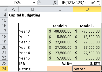
In cell C24, enter the formula
=IF(C23>D23,"better","")
and in cell C25, enter the formula
=IF(D23>C23,"better","")
You can play with the numbers and display information in the evaluation line.
Tip
If the viewer is not concerned with the basic Excel IRR calculation, you can use conditional formatting instead of the evaluation line.
In this next example, a discount is calculated. Assume that a wholesaler offers the following discounts for a product with a basic price of $1.50: 5 percent for 10 items, 10 percent for 100 items, and 20 percent for 1,000 items (see Figure 9-4). The discount should apply to the entire batch and not only to the items above the minimum number.
A possible Excel solution uses the IF() function in a formula to calculate the total price of any number of items (cell C29 contains the item number):
=(1-IF(C29>=1000,20%,IF(C29>=100,10%,IF(C29>=10,5%,0))))*C29*1.5
However, this formula is not flexible. You should create a table displaying the minimum number of items and the discounts, and allocate a cell for the item price.
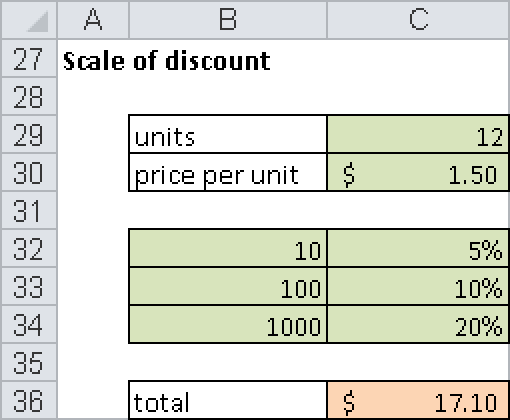
The formula
=(1-IF(C29>=B34,C34,IF(C29>=B33,C33,IF(C29>=B32,C32,0))))*C29*C30
is more complex but allows flexible item numbers, prices, and discounts.
Many nested IF() conditions can quickly become confusing and therefore error prone. You could also use the VLOOKUP() function:
=(1-VLOOKUP(C29,B32:C34,2,TRUE))*C29*C30
This formula requires cells B32 through B34 to contain the minimum item numbers and cells C32 through C34 to contain the discounts. The range B32:C34 is the array used in the VLOOKUP() function, and 2 is the number of the column that contains the return values. You search for the content of C29 in the first column of the array. The logical value TRUE indicates that the search doesn’t need to return an exact match, and the value closest to the required value is returned.