
Syntax. HLOOKUP(lookup_value,table_array,row_index_num,range_lookup)
Definition. This function looks for a value in the top row of a cell range or in an array constant. Depending on the passed arguments, the function returns an entry in the references table.
Arguments
lookup_value (optional). Must evaluate as text, a number, or a logical value. This is the value you search for in the top row of the array.
table_array (required). A reference to a (named) cell range or an array constant (numbers and text must be in braces).
row_index_num (required). Must evaluate to a positive integer not greater than the number of rows in table_array. This argument indicates the number of the row from which the information is returned.
range_lookup (optional). Expects a logical value. The logical value determines whether an exact match should be found (=FALSE) or not (=TRUE or omitted) in the first row.
Background. The HLOOKUP() function begins by searching the first row in the table for the lookup_value. If the range_lookup has been set to FALSE, the function will search the first row for an exact match. If no match is found, you will get the #N/A error. The table does not need to be sorted.
If the range_lookup has been set to TRUE or has been omitted, the function will return an exact match if one exists. Otherwise it will return a value less than the lookup_value. This is used mainly to return values within ranges. In this case, it is important that the lookup table is sorted, so that if the first row displays the lower value in a range, the HLOOKUP() function will select the correct range for the lookup.
Example. You might occasionally have to look for values in cross tables in the left column, based on the values in the header. Figure 10-2 shows an example that uses a time table. Assume that you want to calculate the minutes based on a bus stop and a time.
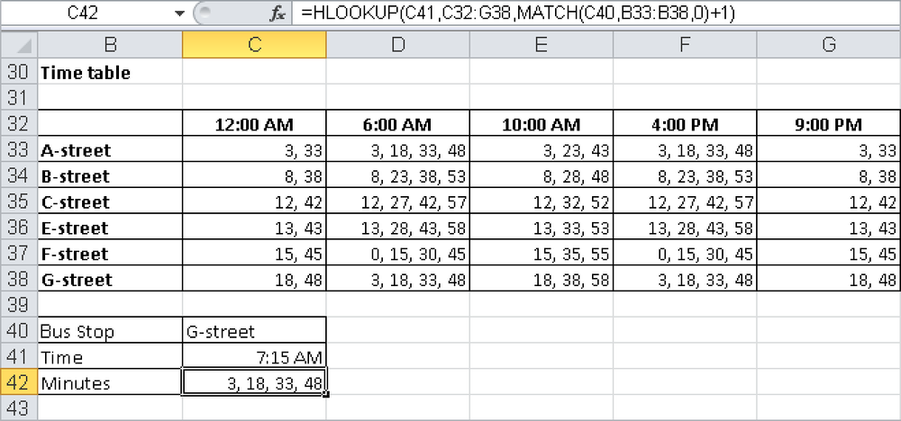
HLOOKUP() cannot do this by itself, because the row containing the stop has to be specified. The combined formula
=HLOOKUP(C41,C32:G38,MATCH(C40,B33:B38,0)+1)
returns the correct result. MATCH() finds the stop in C40 in the first column; adding 1 to this value includes the header in the search array.