
Syntax. VLOOKUP(lookup_value,table_array,col_index_num,range_lookup)
Definition. This function looks for a value in the leftmost column of a table and returns a value in the row selected, as specified by the col_index_num argument. The range_lookup argument determines the type of match required.
Arguments
lookup_value (required). Can be evaluated as text, a number, or a logical value. This is the value you search for in the first column of the table.
table_array (required). A reference to a cell range or an array constant (numbers and text must be in braces).
col_index_num (required). Must evaluate to a positive integer and indicates the number of the column from which the information is returned. The leftmost column in the table is column 1.
range_lookup (optional). A logical value. If this argument evaluates to TRUE (or is omitted), the function searches for the closest match for the lookup_value. FALSE requires an exact match.
Background. The VLOOKUP() function begins by searching the first column in the table for the lookup_value. If the range_lookup has been set to FALSE, the function will search the first column for an exact match. If no match is found, you will get the #N/A error. The table does not need to be sorted.
If the range_lookup has been set to TRUE or has been omitted, the function will return an exact match if one exists. Otherwise it will return a value less than the lookup_value. This is used mainly to return values within ranges. In this case, it is important that the lookup table is sorted, so that if the first column displays the lower value in a range, the VLOOKUP() function will select the correct range for the lookup.
Examples. The following examples illustrate how to use the VLOOKUP() function.
Combining with Other Functions. The second example of the INDEX() function uses the VLOOKUP() function to find an exact match for a value.
See Also
The sections describing the ISERROR() and ISNA() functions in Chapter 11, contain more examples. The examples for the IF() function in Chapter 9, include an example for discounts.
VLOOKUP() returns only the values to the right of the search column. If you want to locate values more generally across a table, use the INDEX() and MATCH() functions.
Assume that you have a list in which numbers are assigned to text (see Figure 10-11).
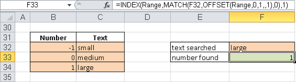
The range from B32 through C34 has the name Range. You want to determine the number assigned to small. You can also do the inverse, that is, find the word assigned to the number, which is no problem with VLOOKUP():
=VLOOKUP(-1,Range,2,FALSE)
This formula will search for –1 in the leftmost column and return small, but searching the other way around, for example, for the number associated with the text large, is more complicated. The following formula offers a solution:
=INDEX(Range,MATCH(F32,OFFSET(Range,0,1,,1),0),1)
With OFFSET(), you define the second column of the range as the column that is searched. MATCH() returns the row in the range containing the value in cell F32. INDEX() takes this row number and uses column number 1.