
Note
In Excel 2010, the FDIST() function was replaced with the F.DIST.RT() function, and the F.DIST.RT() function was added to increase the accuracy of the results. To ensure the backward compatibility of F.DIST.RT(), the FDIST() function is still available.
Syntax. F.DIST.RT(x,degrees_freedom1,degrees_freedom2)
Definition. This function returns the values of a distribution function (1 alpha) of a right F-distributed random variable. Use this function to determine whether two data sets have different variances. For example, you can compare the survey results of three equal employee groups to determine whether the variance or results are different.
Arguments
x (required). The value at which to evaluate the function
degrees_freedom1 (required). The degrees of freedom in the numerator
degrees_freedom2 (required). The degrees of freedom in the denominator
Note
If one of the arguments isn’t a numeric value, the F.DIST.RT() function returns the #VALUE! error.
If x is negative, F.DIST.RT() returns the #NUM! error value.
If degrees_freedom1 or degrees_freedom2 isn’t an integer, the decimal places are truncated. If degrees_freedom1 is less than 1 or degrees_freedom2 is greater than or equal to 1010, the function returns the #NUM! error. If degrees_freedom2 is less than 1 or degrees_freedom2 is greater than or equal to 1010, the function returns the #NUM! error.
F.DIST.RT() is calculated as F.DIST.RT = P(F>x) where F is an F-distributed random variable with degrees_freedom1 and degrees_freedom2.
Background. The F.DIST.RT() function returns the significance level based on a value. The F.DIST.RT() function calculates the probability—that is, the significance level—for the critical values calculated by F.INV.RT().
The F.INV.RT() function calculates the critical F-value based on the probability and degrees of freedom and requires the probability argument.
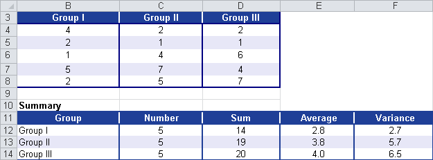
Example. Let’s use the example for F.INV.RT(). In a survey, 15 employees had to answer 10 questions. Each question had three possible answers, as shown in Figure 12-41.
The null hypothesis indicates that there is no difference between the three groups. However, the alternative hypothesis assumes the opposite. A simple variance analysis returns the results shown in Figure 12-42.
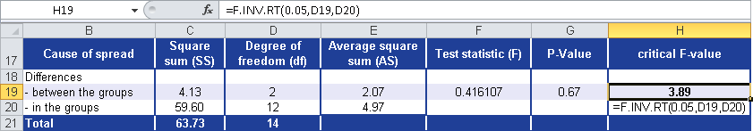
With the F.INV.RT() function and a significance level (probability) of 0.05, you calculate a critical F-value of 3.89. The F.DIST.RT() function returns a significance level of 0.05.
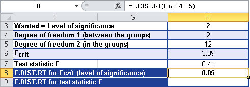
The example uses the values shown in Figure 12-43 to calculate F.DIST.RT().

The calculation of the significance level for F returns the result shown in Figure 12-44.
The F.DIST.RT() function returns a probability of 0.67 (67 percent) for statistic F = 0.4161 (see Figure 12-45).
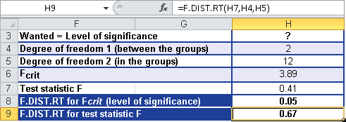
Because the significance level a is greater than the statistic F, the null hypothesis is confirmed. This means that you can assume that there is no significant difference between the two groups.