
Syntax. NORM.DIST(x,mean,standard_dev,cumulative)
Definition. This function returns the normal distribution for an average value and a standard variance. This function has a very wide range of applications in statistics, including hypothesis testing.
Arguments
x (required). The distribution value (quantile) for which you want to calculate the probability.
mean (required). The arithmetic mean of the distribution.
standard_dev (required). The standard deviation of the distribution.
cumulative (required). The logical value that represents the type of the function. If cumulative is TRUE, the NORM.DIST() function returns the value of the distribution function (cumulative density function). If cumulative is FALSE, the NORM.DIST() function returns the value of the density function.
Note
If mean or standard_dev isn’t a numeric expression, the NORM.DIST() function returns the #VALUE! error. If standard_dev is less than or equal to 0, the function returns the #NUM! error.
If mean = 0, standard_dev = 1, and cumulative = TRUE, NORM.DIST() returns the standard normal distribution.
Background. Excel offers numerous functions to calculate distributions and to evaluate hypotheses. One example is the NORM.DIST() function. In general, distributions help to answer questions regarding probabilities. An example is a coin toss that has only two probabilities: heads or tails.
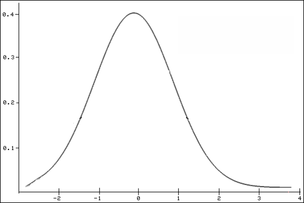
As already mentioned, the NORM.DIST() function returns the normal distribution of given values. The normal distribution is the most important continuous probability distribution that indicates the probability of a value for a random variable x. The probability density is also called the Gaussian function, Gaussian curve, Gaussian bell, or bell curve and is shown in Figure 12-102.
The special meaning of the normal distribution is based on the central limit theorem that states that a sum of n independent identical distributed random variables is normal distributed at the limit.
The normal distribution explains many scientific processes exactly or approximately—especially processes that work independently of each other in different directions.
Unlike the binomial distribution, the normal distribution is symmetrical (as shown in Figure 12-102). This means that the normal distribution is similar to a bell curve where the smallest and largest value have the lowest probability and the mean value has the highest probability.
Note the following for a normal distribution:
It is bell-curved.
It is unimodal.
It comes asymptotically close to the x axis.
It is symmetrical.
The following statements are also true:
The maximum is at the arithmetic mean.
Each 50 percent of the range is two-tailed to the arithmetic mean.
The arithmetic mean and median are congruent.
The mode, median, and arithmetic mean are congruent.
The inflection points are at the mean value plus standard deviation and at the mean value minus standard deviation.
Excel offers two functions for most distributions. A function that calculates a distribution and ends in DIST calculates the probability for a certain value. The associated inverse function, ending in INV, calculates the value for a certain probability.
Note
The NORM.INV() function accepts a probability, a standard deviation, and a mean value as arguments.
The equation for the density function of the normal distribution (cumulative = FALSE) is:
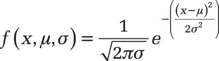
If cumulative = TRUE, the formula returns the integral of the given formula from negative infinity to x.
Example. You are a light bulb manufacturer and want to analyze the performance of light bulbs. You also have calculated the average life cycle and the associated standard deviation. You want to know the probability for the light bulbs to last longer or less long when used daily. For this calculation, you use the NORM.DIST() function. The life cycle of your light bulbs is normal distributed with:
An average of 2,000 working hours = arg-hour average
A standard deviation of 579 hours = argument StdDev
To calculate the distribution function, you specify the logical value TRUE for the cumulative argument. If you want to calculate the density function, use the logical value FALSE.
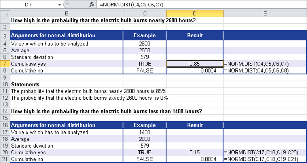
You ask the following question: How high is the probability for a light bulb to work up to 2,600 hours or only up to 1,400 hours? And how high is the probability that exactly these hours will be reached?
The values 2,600 hours and 1,400 hours are indicated by the x argument. They are the values within the distribution that you want to calculate the probability for. Figure 12-103 shows the results.
What conclusions can you draw from these results?
The probability for a light bulb to work up to 2,600 hours is 85 percent.
The probability for a light bulb to work exactly 2,600 hours is 0.04 percent.
The probability for a light bulb to work only 1,400 hours is 15 percent.
The probability for a light bulb to work exactly 1,400 hours is 0.04 percent.
In this way you, can perform numerous calculations, test hypotheses, and specify the probabilities for characteristics in intervals.