To make data easier to interpret, use the conditional formatting feature to automatically format the data. With conditional formats, values are selected if they meet certain criteria, and the cell range is formatted accordingly. Conditional formats visually highlight the distribution and variation of data.
With regard to our example, the condition could be “Format in green all cells in the Profit Margin column that contain a value of at least $200,000.” To enter this format, perform the following steps:
Select the cell range in the Profit Margin column.
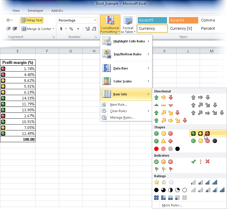
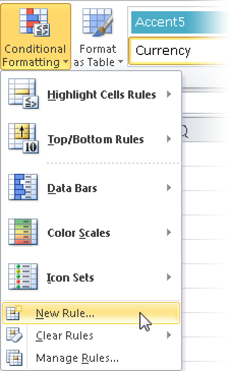
Click the Conditional Formatting button in the Style group on the Home tab, and then click New Rule (see Figure 1-32).
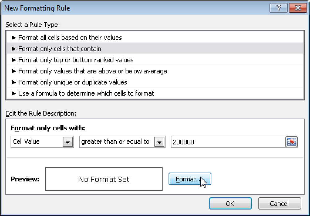
In the New Formatting Rule dialog box, under Select A Rule Type, select Format Only Cells That Contain.
Specify the settings in the Edit The Rule Description pane. Select Cell Value and Greater Than Or Equal To in the list boxes.
Enter the value 200000 in the third field (see Figure 1-33).
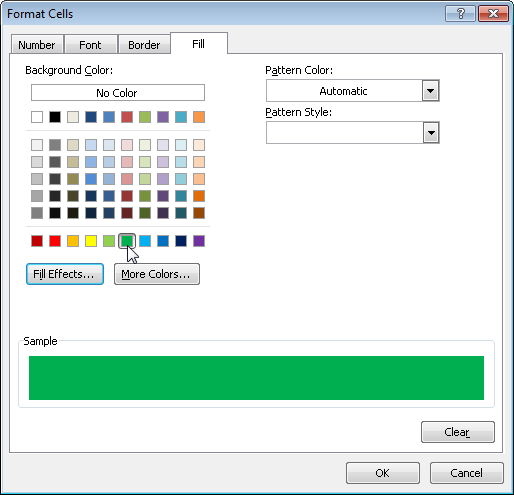
Click the Fill tab of the Format Cells dialog box, and select a background color (see Figure 1-34).
Click OK twice to confirm your selection. The values in the Profit margin column are displayed in the color you selected if the condition is met (see Figure 1-35).
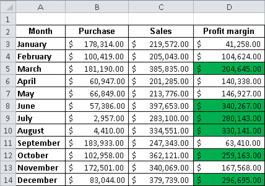
You can use conditional formatting to automatically display the values in your table in different colors to give them significant visual impact.
You can also use other color fill options or an icon set to format cells. Conditions can apply to text, numeric, date, or time values, as well as to values that fall below or above the average.
Data bars are also a quick way to visually highlight values in tables (see Figure 1-36).
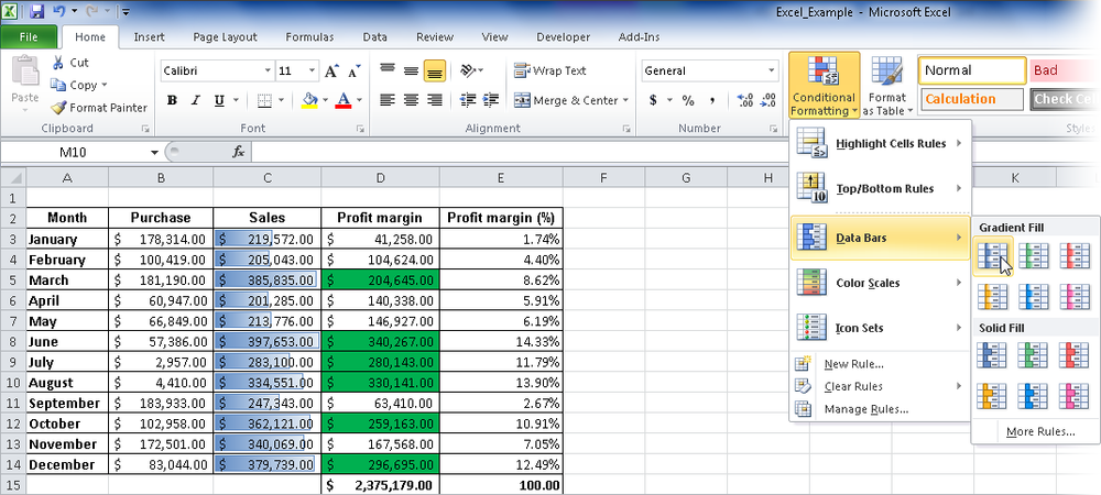
There are many different options to choose from.
Tip: Apply conditional formats to highlight data
In Excel 2007 and Excel 2010, conditional formats have improved significantly (see Figure 1-37). Now you can add not only colors but also arrows, traffic lights, and other icons. This functionality is also referred to as KPI (Key Performance Indicators).