PivotTables help you arrange and consolidate data into well-defined tables. With a PivotTable, you can easily generate cross-tabulations and analyze information by rotating and moving column and row selections and by filtering. The original data remains unchanged, and the PivotTable is quickly generated even with large amounts of data. In Excel 2007 and Excel 2010, PivotTable data can also easily be displayed as a PivotChart.
Tip
A PivotTable is useful for quickly obtaining summary information from long lists or large amounts of data.
To create a PivotTable, perform the following steps:
Open the Excel_Pivot_Data.xlsx file from the sample files.
In the table, select the cell range for which you want to create the PivotTable. In this case, select cell A1 (Customer Name) through cell J100 (Total Price), or select the entire table by pressing Ctrl+A from anywhere within the table.
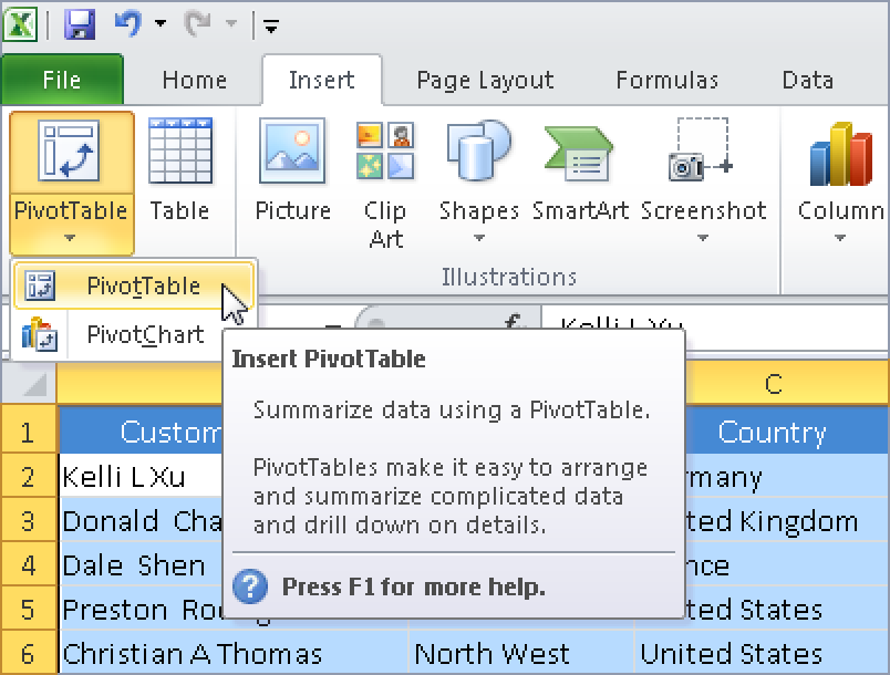
On the Insert tab, in the Table group, click the arrow on the PivotTable button and select PivotTable (see Figure 1-52).
Tip: Find Pivot functions on the Insert tab
In Excel 2003, the Pivot functions were located on the File menu. In Excel 2007 and Excel 2010, you can open the Pivot functions by clicking a button on the Insert tab. The functions open in a separate tool window as soon as you start creating a PivotTable.
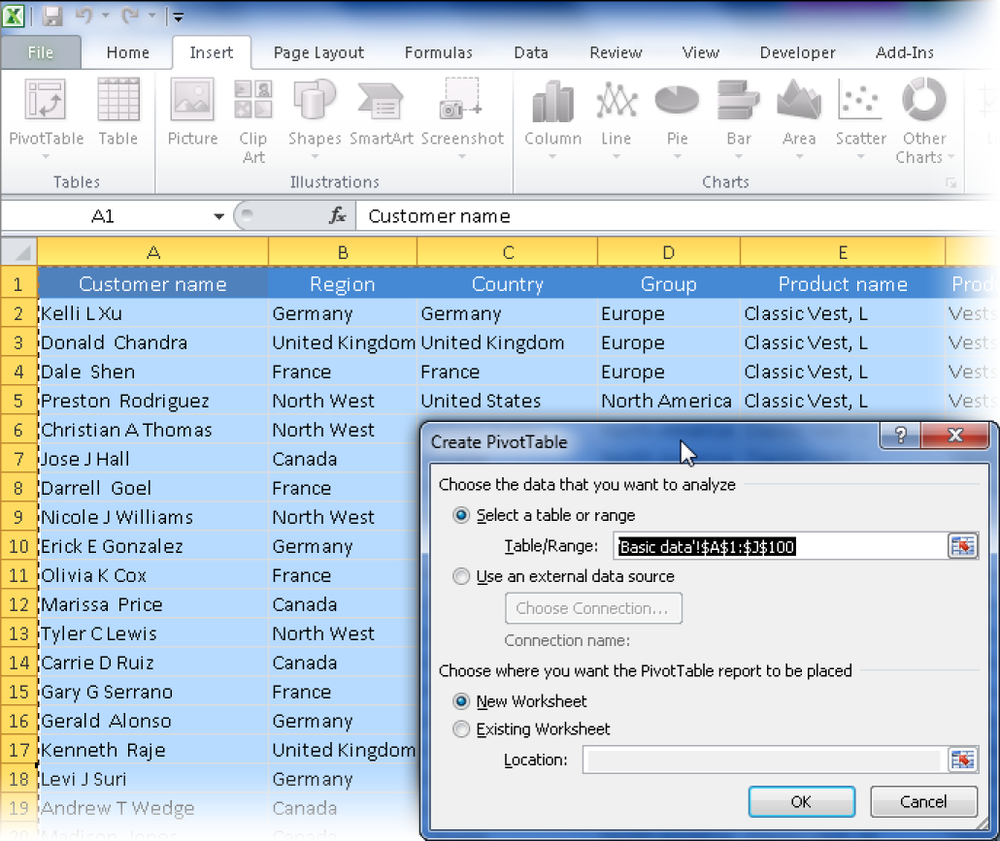
Because you have already selected the data, the PivotTable range is displayed in the Select Table Or Range box in the PivotTable dialog box.
Select an option under Choose Where You Want The PivotTable Report To Be Placed. Selecting the New Worksheet option is recommended (see Figure 1-53).
Click OK. The PivotTable framework is displayed.
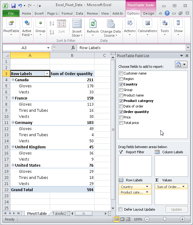
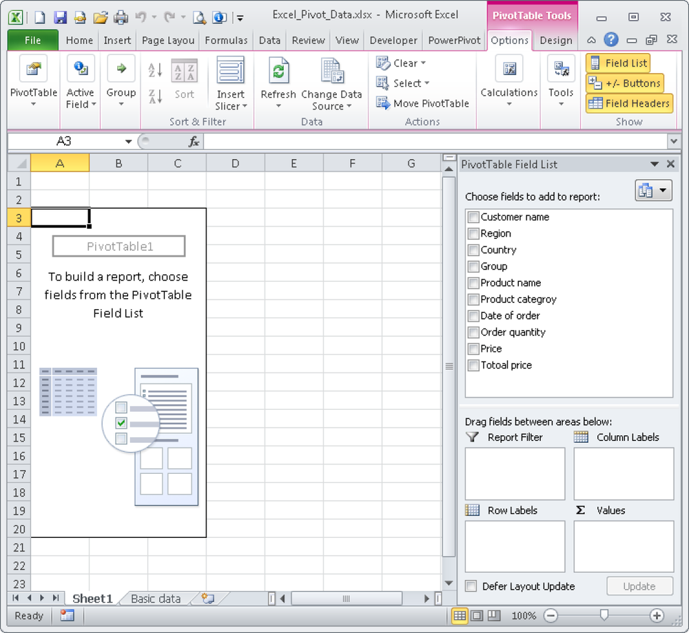
An empty PivotTable report is added, in this case in a new worksheet, and the PivotTable field list is displayed. In this list, you can select fields, create a layout, and change the PivotTable report.
You can also use the PivotTable tools on the PivotTable Tool contextual tab, which you can access from the ribbon (see Figure 1-54).
The following example illustrates the functionality of a PivotTable. Assume that you want to find out in which country the most orders for gloves are placed. For this you need the PivotTable fields Country, Product Category, and Order Quantity.
Follow these steps:
Select the Country, Product Category, and Order Quantity check boxes in the PivotTable field list.
After you have enabled the fields, the associated data are automatically positioned in the default range of the layout, but you can move the fields to any position (see Figure 1-55).
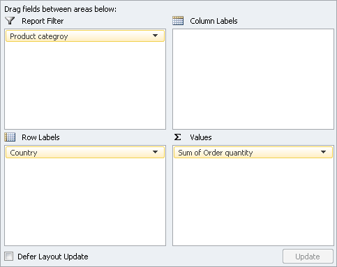
Because you want to view the order quantity for gloves per country, you should move the Product Category column into the Report Filter area. This will allow you to filter by country. Drag the Product Category field into the Report Filter area within the PivotTable field list (see Figure 1-56).
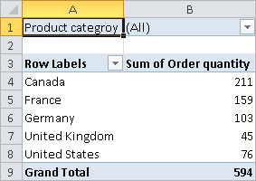
As soon as you release the mouse button, the data is arranged in the PivotTable (see Figure 1-57).
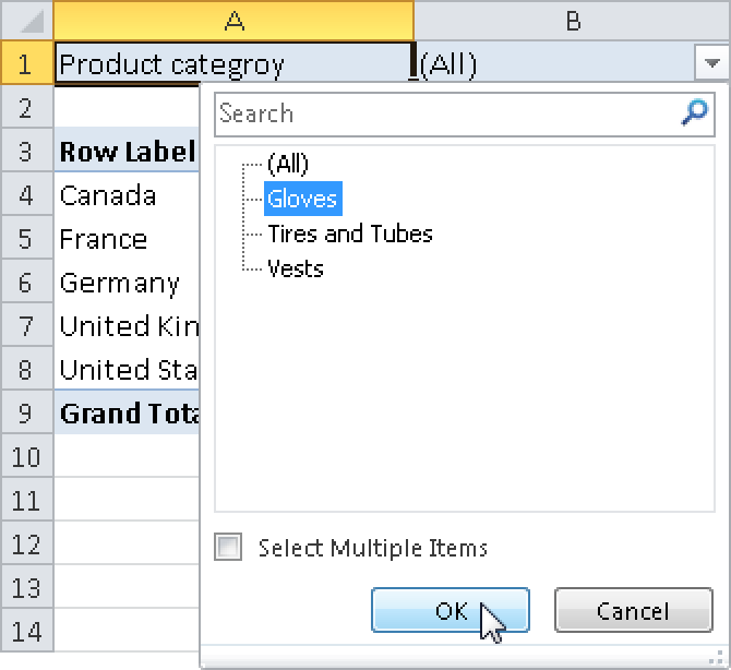
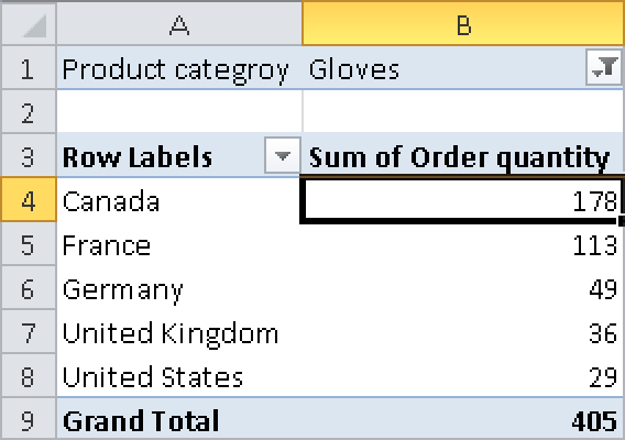
In the (All) list, select Gloves and click OK (see Figure 1-58).
Only the order quantities for gloves in the individual countries are displayed (see Figure 1-59). Canada is the frontrunner!