
Syntax. T.TEST(array1,array2,tails,type)
Definition. This function returns the test statistic of a Student’s t-test. Use TTEST() to check whether two samples are likely to have come from the same two populations that have the same mean.
Arguments
array1 (required). The first data set.
array2 (required). The second data set.
tails (required). Specifies the number of distribution tails. If tails = 1, the T.TEST() function uses the one-tailed distribution. If tails = 2, the T.TEST() function uses the two-tailed distribution.
type (required). The type of t-test to perform:
If type equals 1, the test is paired.
If type equals 2, the two-sample equal variance (homoscedastic) test is performed.
If type equals 3, the two-sample unequal variance (heteroskedastic) test is performed.
Note
If array1 and array2 have a different number of data points and type = 1 (paired), T.TEST() returns the #N/A error.
The tails and type arguments are truncated to integers. If tails or type isn’t a numeric value, the T.TEST() function returns the #VALUE! error.
If tails is any value other than 1 or 2, T.TEST() returns the #NUM! error.
The T.TEST() function uses the data in array1 and array2 to calculate a nonnegative t-statistic value. If tails = 1, T.TEST() returns the probability of a higher value of the t-statistic value under the assumption that array1 and array2 are samples from populations with the same mean. The value returned by T.TEST() when tails = 2 is double that returned when tails = 1 and corresponds to the probability of a higher absolute value of the t-statistic under the “same population means” assumption.
Background. The t-distribution functions indicate whether one or two samples correspond to the normal distribution. For example, you can test whether a treatment method is better than another.
The t-distribution belongs to the probability distributions and was developed in 1908 by William Sealey Gosset (alias “Student”). William Gosset found out that standardized normal distributed data are no longer normal distributed if the variance of the characteristic is unknown and the sample variance has to be used for an estimate.
The t-distribution is independent from the mean μ and the standard deviation s and only depends on the degrees of freedom.
Note
The t-distribution is similar to the standard normal distribution. Like the standard normal distribution, the t-distribution is consistent, symmetrical, and bell-shaped, and has a variance range from plus/minus infinity.
Because the normal distribution applies only to a large amount of data, it usually has to be corrected. This uncertainty is observed in a t-distribution by the symmetrical distribution. If there are high degrees of freedom, the t-distribution transitions into the normal distribution.
The lower the degrees of freedom, the further away are the integral limits from the mean based on a given probability and fixed standard deviation such that for a two-tailed test, the interval is greater than 1.96 (for P = 0.95).
The t-distribution describes the distribution of a term:
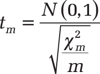
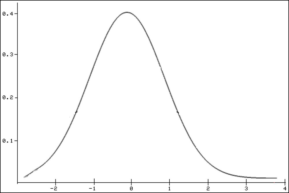
N(0.1) is a standard normal distributed random variable and a χ2-distributed with m degrees of freedom. The counter variable has to be independent from the denominator variable. The density function of the t-distribution is symmetrical based on the expected value 0 (see Figure 12-141).
The t-test allows hypotheses for smaller samples if the population shows a normal distribution, a certain mean is assumed, and the standard deviation is unknown.
There are three types of t-tests:
Comparison of the means from the sample with the mean from the population. An example is the comparison of the average age of the population in New York with that of the population in the entire United States.
Mean comparison from independent samples An example is the comparison of the average income of men and women in New York. Because the variances of the two populations from which the samples were obtained are unknown, the variances from the sample are estimated. The t-distribution is followed by a t-test with k degrees of freedom.
Comparison of the sample means from interdependent samples. An example is the comparison of the education of spouses. A characteristic of a sample is evaluated twice and tested if the second value is higher (or lower) than the first value. The t-distribution is followed by a t-value with n –1 degrees of freedom. N is the number of the value pairs.
The question the t-test answers is: What is the probability that the difference between the means is random? And what is the probability for an alpha error if, based on the different means in the sample, you assume that this difference also exists in the population?
Note
The alpha error (also called alpha risk) is the probability that a characteristic of the data is random. The alpha error is often 10 percent, 5 percent, or less than 5 percent (significance level) and seldom larger than 10 percent.
In other words, the t-test evaluates the (error) probability of a thesis based on samples–that is, it evaluates the probability for an alpha error.
Types of t-Tests. There are two general distinctions between the different t-test types::
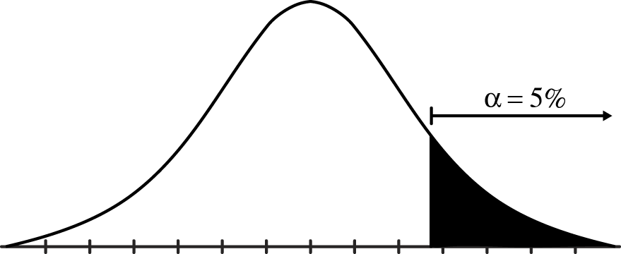
One-tailed t-test For a one-tailed t-test, directional hypotheses are prepared. Where H0 and H1:
H0: μ1– μ2 less than or equal to 0
H1: μ1 – μ2 greater than 0
To reach a conventional alpha level (significance level) of 5 percent, t has to be positioned on the predicted side of the t-distribution in the 5 percent range (see Figure 12-142).
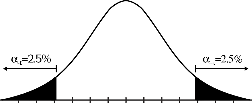
Two-tailed t-test. For a two-tailed t-test, nondirectional hypotheses are prepared. Where H0 and H1:
H0: μ1 – μ2 = 0
H1: μ1 – μ2 ? 0
To reach an overall alpha level (significance level) of 5 percent, t has to be positioned in the lower or upper 2.5 percent range (see Figure 12-143).
The following is true for one-tailed t-tests versus two-tailed t-tests:
For a two-tailed test, t has to have a higher value to be significant (α=0.05).
For a two-tailed test, t is assigned a higher error probability than for a one-tailed test.
x1–x2 is more likely to be significant in a one-tailed test than in a two-tailed test.
A one-tailed test has a higher test performance.
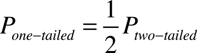
For a two-tailed test, usually the t-value is assigned double the p-value that is assigned for a one-tailed test. This p-value can be converted into the p-value for a one-tailed test (and vice versa).
This results in the following formulas:
Example. The compatibility of a drug was examined in a clinical study. You have the test results as well as some explanations. One test group took the normal daily dosage, and the other test group took an increased dosage at the beginning of the study. One person had to cancel the test early for private reasons. The goal was to determine whether the increased dosage accelerates the healing process. The duration of treatment was calculated in days.
The null hypothesis indicates that there is no difference in the two test groups regarding the success of treatment. The alternative hypothesis indicates that the second group recovered faster because the method of treatment is more efficient than the usual treatment. You have to analyze the test results to determine whether the null hypothesis can be accepted or has to be rejected.
Because you weren’t present during the test and don’t have all the background information, you want to calculate the probability that the means of the two samples are equal by using the T.TEST() function. By comparing the result with the significance level, you can draw a conclusion about the null hypothesis.
You run a one-tailed, type 2 t-test; that is, you compare the mean of two independent samples. The significance level is 5 percent. The following formula calculates the statistic t:
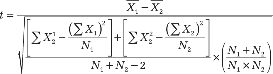
The x-values are the means of Group 1 and Group 2; N1 and N2 indicate the size of the two samples. Figure 12-144 shows the result of the study.
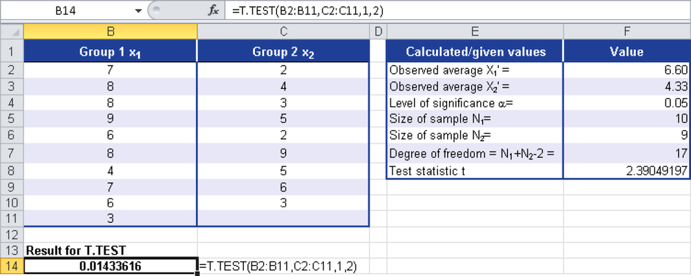
Because T.TEST() returns a probability value, the result is 1.4 percent. Now you can assume with a 1.4 percent probability that the sample means are not equal. In other words: You can say with 1.4 percent certainty that the samples are unequal. This is already shown in cells F2 and F3 in Figure 12-144. However, these are only estimated values based on samples.
Because the result for T.TEST() is < α, the null hypothesis has to be rejected. This means that the statement that there is no difference in the two test groups regarding the success of treatment is disregarded.