
Microsoft Excel saves dates as continuous numbers so that they can be used in calculations. By default, Excel determines a date based on continuous numbers starting at 1, which is January 1st, 1900, and ending with the number 2,958,465, which is December 31st, 9999. This means that Excel can calculate date values only between these two dates.
Caution
Microsoft Excel for Mac uses a different date system. The calendar starts at 01/01/1904. For compatibility reasons, the Windows version of Excel provides an option for working with the date system starting at 1904. Select this option only if you have to change worksheets between Windows and Mac computers. But be careful: This setting applies to the active worksheet, and the dates already entered will be changed!
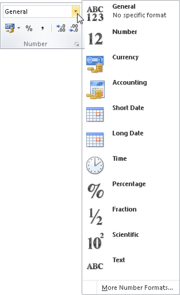
To display the continuous number for a date or time value, restore the General format of the cell. In versions of Excel before Excel 2003, you can select the Delete option on the Edit menu and click Formats to restore the General format. In Excel 2007 or Excel 2010, you only need to click the number format on the Home tab (see Figure 2-1).
Here is how dates and times together are displayed as continuous numbers: The number before the period is the date. For example, the number 39448 indicates the number of days since 01/01/1900. The result is January 1st, 2008. The numbers after the period indicate the time. If you divide this value by the number of hours in a day, you get the decimal fraction for an hour: 1/24 = 0.04166667. The number 0.5 indicates that half a day has passed and it is noon. The number 0.25 indicates 6:00 A.M., and 0.75 indicates 6:00 P.M.
You can view the date and time by using the formats listed in Table 2-1. The example worksheets for Chapter 7, include many more examples of formats.
Table 2-1. Number Formats for Dates and Times
Format | Description/Result |
|---|---|
Number | =SUM(number1,number2...) |
Text | =CONCATENATE(Text1,Text2,...) |
T | Day without leading zero |
TT | Day with leading zero for one-digit numbers |
TTT | Abbreviated name of the day (Mo, Tu, We, Th, Fr, Sa, Su) |
TTTT | Name of the day (Monday, Tuesday, and so on) |
M | Month without leading zero |
MM | Month with leading zero for one-digit numbers |
MMM | Abbreviated name of the month (Jan, Feb, Mar, and so on) |
MMMM | Name of the month (January, February, March, and so on) |
J or JJ | Two-digit year |
JJJ or JJJJ | Four-digit year |
h | Hour without leading zero |
hh | Hour with leading zero |
m | Minute without leading zero |
mm | Minute with leading zero |
[h] or [hh] | Hours for more than 24 hours |
[m] or [mm] | Minutes for more than 60 minutes |
[s] or [ss] | Seconds for more than 60 seconds |
hh:mm AM | Twelve-hour format (A.M.): Ante meridian (Latin for “before noon,” the hours between midnight and noon) |
hh:mm PM | Twelve-hour format (P.M.): Post meridian (Latin for “after noon,” the hours between noon and midnight) |
When programming date calculations, you have to consider leap years. In the Gregorian calendar, every fourth year is a leap year in which the month of February has 29 days. If the year can be divided by 100 without a remainder, the year isn’t a leap year, with one exception: If the year is divisible by 400 without a remainder, the year is a leap year anyway. If this last rule is disregarded, there will be further mistakes instead of a 29th of February.
Though most of these date and time functions are available with the standard Excel 2003 installation (and earlier), some need to be enabled. You can enable them by selecting Tools/Add-Ins and making a selection in the Add-Ins dialog box (see Figure 2-2).
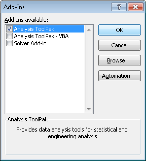
Figure 2-2. In Excel 2003 and earlier, certain analysis functions have to be enabled in the Add-Ins dialog box.
In Excel 2007 and Excel 2010, you can use all functions without having to enable the add-in.
The following practice examples show typical calculations that use the date and time functions of Excel.
Assume that Daylight Saving Time starts on the last Sunday in March and ends on the last Sunday in October. The start of Daylight Saving Time in the current year is calculated with the following formula:
=DATE(YEAR(TODAY()),4,)-WEEKDAY(DATE(YEAR(TODAY()),4,))+1
DATE(YEAR(TODAY()),4,) returns March 31st of the
current year. WEEKDAY(DATE(YEAR(TODAY()),4,)) returns the weekday number of March
31st in the current year. So by subtracting this value from the last day
of the month and adding one day, you get the date of the last Sunday of March.
The following formula returns the end of Daylight Saving Time for the current year (the last Sunday of October):
=DATE(YEAR(TODAY()),11,)-WEEKDAY(DATE(YEAR(TODAY()),11,))+1
You can use a nested date function to find out the continuous number of today’s date:
=TODAY()-DATE(YEAR(TODAY())-1,12,31)
This formula subtracts December 31st of last year from today’s date. The result is the difference between both dates in days—in this case, the number of the day for today in the current year.
Enter the current time by pressing Ctrl+Shift+: (colon). The time is displayed in the hh:mm number format. For example, the cell might display 2:25 P.M., and the formula bar would also show 2:25 P.M. If you select the General number format, the value (in this example, 0.60069444) is displayed. If you are calculating times, you should remember that the time is always a value from 0 through 1.
Usually you don’t have to take care of the conversion, because Excel automatically converts dates and times. To calculate the difference between two date and time entries, you can subtract the start date/time from the end date/time. This way, you can create a table with working hours to calculate the hours for each working day, as in the example that follows in the next section.
Assume that you want to create a worksheet with shift work hours. Some employees work from 10:00 P.M. to 6:00 A.M. How do you calculate the correct working hours?
If the employees work from 10:00 P.M. to 6:00 A.M., and you calculate the difference, the result is ######. Even if you change the column width, the problem is not solved. If, however, you change the format of this number to General, the value is displayed. It is interesting that Excel can calculate the time when you set the number format to General, but not when it is set to a time format. As you can see, the Excel time format does not work with negative numbers.
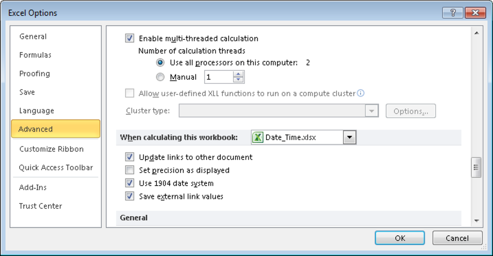
You have two options for solving this problem: Change the general setting to the 1904 date system (see Figure 2-3), or use a formula.
Caution
Use the Tools/Options menu command (Excel 2003 or earlier) to select the 1904 date system check box on the Calculation tab. With this option enabled, Excel can perform calculations with negative times. However, this has disadvantages: This setting applies only to the active worksheet. If other worksheets refer to these time values, you must change those worksheets accordingly. All entered date values change by four years, and you must change all existing dates. Therefore, this option isn’t a reliable solution.
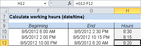
To calculate a time interval that crosses over to another day, you can enter the times and include the date. If work begins at 8/4/2008 10:00 P.M. and ends at 8/5/2008 06:20 A.M., you can easily calculate the difference. This is done with the formula =End-Beginning. However, you should display the number format of the result cell in the hh:mm format (see Figure 2-4).
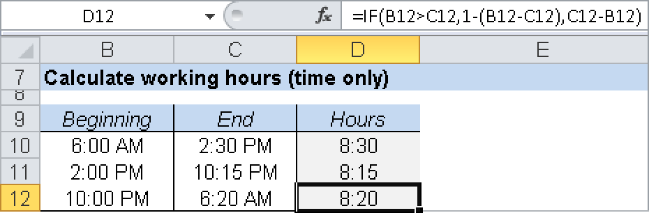
Another approach is to check which time value is higher if the times are available for the beginning and end. With the logical IF(test;value_if_true,value_if_false) function, you get the result with the formula
=IF(Beginning>End,1-(Beginning-End),End-Beginning)
This formula can be used to calculate the difference up to 24 hours. Figure 2-5 shows an example.
If the time intervals are less than 24 hours, and the start time is greater than the end time, you could take the absolute difference between the two times and then subtract this from 1.
=If(Beginning>End,1-(Beginning-End), End – Beginning)
Another option is to insert a comparison of Beginning>End. The result is one of the two logical values TRUE or FALSE. If Excel finds a logical value in a calculation, the value is converted into 1 or 0. Because an entire day corresponds to the value 1, you can add 1 to a time (when the beginning is larger than the end) and get the result in the next day. Use this formula:
=(Beginning>End)+End-Beginning
When adding times, you need to be aware of several factors. In Excel, the addition of two times will not exceed 24 hours; the result of 15 hours plus 12 hours is 3 hours. You can resolve this problem by using the correct number format:
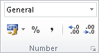
Select the result cell and click the Format/Cells menu option (Excel 2003 and earlier), or click the arrow in the lower-right corner of the Number group on the Home tab (Excel 2007 and Excel 2010), as shown in Figure 2-6.
Click the Number tab of the Format Cells dialog box, and select Custom in the Category list field.
Select the number format [h]:mm. Pay attention to the brackets. If you cannot find the exact format, just modify a similar entry.
The result is displayed in the 24:00 format.
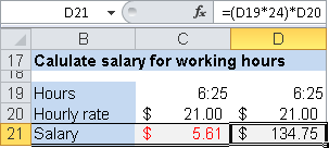
Because Excel treats hours as fractions of a day, you have to be careful when calculating values based on the number of working hours. For example, if an employee works 6.25 hours and is paid $21 per hour, and you simply multiply these values, the result is only $5.61. The employee would not be happy with this amount.
To calculate the correct result, you have to multiply the number of hours by 24. The correct calculation would be =(“6:25”*24)*21 resulting in $134.75 (see Figure 2-7).
Because the exact minute or second is not always needed, you can round time values. Remember that Excel uses the value 1 for a day. An hour is a fraction of a day, or 1/24, and a minute is 1/1440. If you set these values as the arguments of the MROUND() table function, the time is rounded accordingly.
Suppose, for example, that cell B42 contains the time 08:52:36 in the number format hh:mm:ss. The formula =MROUND(B42,1/24) results in 09:00:00, and the formula =MROUND(B42,1/1440) in 08:53:00.
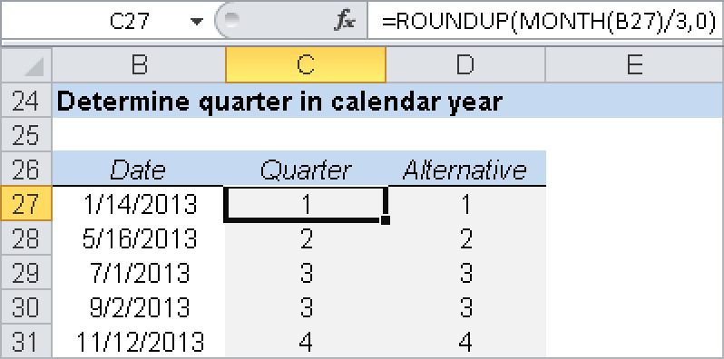
Supposed you want to identify which quarter of the year a given date falls in. For this example, the first quarter includes January through March, the second April through June, and so on.
Divide the number of the month by 3, and round the result to the next integer in the formula =ROUNDUP(MONTH(date value)/3,0) as shown in Figure 2-8.
You may want to convert a time into decimal hours and minutes. If the hours and minutes are integers, use the following formula to calculate the decimal hours:
Time = Hour(date value) + Minute(date value)/60
If the time is shown as a fraction, multiply this value by 24. Here are some examples:
06:30 is 6.5 decimal hours.
07:15 is 7.25 decimal hours.
09:45 is 9.75 decimal hours.