
The database functions are particularly useful because they analyze data from tables with headings (field names) and data rows (data records). The block of information in rows and columns constitutes a database.
Using the database functions is made easier if the following rules are observed:
Make sure lists have column headings.
Make sure lists don’t contain empty rows or columns.
Make sure lists don’t contain linked cells.
In Excel 2003 and earlier, the usage of Excel as a database was stretched to its limits pretty quickly because a table was limited to 65,536 rows. In Excel 2007 this limit was extended: Now each table for data lists can have 1,048,576 rows. The same applies to columns: In Excel 2003, a table could have 256 columns, and in Excel 2007, up to 16,384 columns are allowed.
Dynamic names are an effective way to simplify working with data in Excel databases. If you specify a dynamic name, you can open a data template to view and capture data and then browse the data records, find data, or enter data.
When using dynamic names, it is important to remember to include an empty row below and an empty column next to the last entry. This avoids problems if you add new columns or rows at a later time.
See Also
The OFFSET() function used in the following example is explained in more detail in Chapter 13.
To assign a dynamic name to the Excel list, perform the following steps in Excel 2007 or Excel 2010:
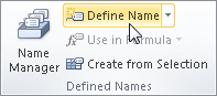
Click in cell A1 or the first cell of your database, and then click the Define Names button (see Figure 2-30) in the Defined Names group on the Formulas tab.
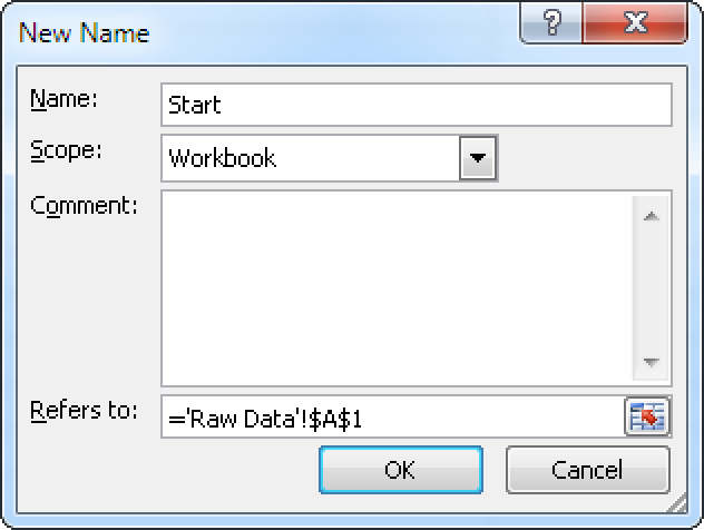
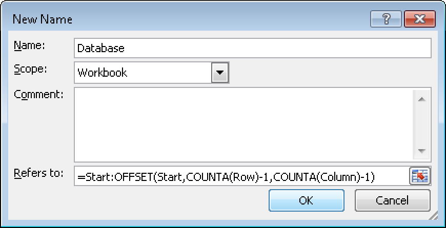
Enter the name Start in the New Name dialog box, and click OK (see Figure 2-31).
The starting point of the database is now set. Next you have to generate the dynamic name of the database with the OFFSET() function. First you have to find out how many entries exist in column A and row 1.
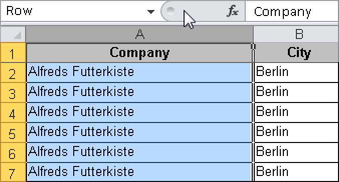
Click the header of column A to select the entire column, and enter the name Row in the name box (see Figure 2-32). Press the Enter key to confirm.
To test the settings, calculate the number of rows in column A by using the COUNTA() function. Click any empty cell in the worksheet and enter the following formula:
=COUNTA(row)Because column A has the name Row, you have to click only column A to select the argument for the function. Because the number of rows was calculated with the COUNTA() function, the content of all cells, including text and logical values, is taken into account.
Press the Enter key to confirm.
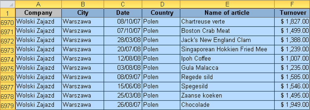
If you are working with the Excel table in the DBFunction empty.xlsx file from the sample files, the result is 7,008. Next you will calculate the number of entries in row 1. To do this you use the same procedure you used to calculate the number of entries in column A.
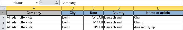
Click the row header to select the entire row, and enter the name Column in the name box (see Figure 2-33).
To test the settings, calculate the number of entries in row 1 by using the COUNTA() function. Click any empty cell in the worksheet and enter the following formula:
=COUNTA(column)
If you are working with the Excel table in the DBFunction empty.xlsx file from the sample files, the result is 6.
By naming the column and row and by calculating the entries within the column and row, you have already created the basis for the dynamic name of the matrix (database). If you add or delete columns or rows, the value within your formula cells will increase or decrease, respectively.
Now you can actually assign a dynamic name to the database in the following range: The database range starts at cell A1, to which you gave the name Start. This position is extended down by the number of rows calculated with the =COUNTA(row) function; in this case, 7,008 entries. At the same time, the position is extended six columns to the right, beginning at the Start cell, based on the result of the calculation
=COUNTA(column)
You then need to subtract one position in each dimension of the database range. The following function assigns the dynamic name and defines the database range:
=Start:OFFSET(start,COUNTA(row)-1,COUNTA(column)-1)
Perform the following steps:
On the Formulas tab, click the Define Name button in the Defined Names group.
In the New Name dialog box, enter the name Database.
Enter in the Refers To field the formula shown just before these steps, as shown in Figure 2-34. If you aren’t using the worksheet in the Chapter02 sample files folder, adjust the entry accordingly.
Click the OK button.
To check the name, press the F5 key and enter the name Database in the Reference field in the Go To dialog box (see Figure 2-35) that appears. Click OK.
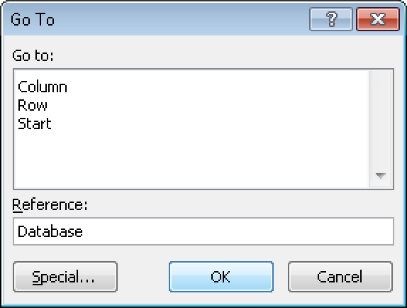
If the dynamic name was assigned properly and the database range is correct, the entire database range between cell A1 and cell F7008 should be selected (see Figure 2-36, but note that only a portion of the range is shown).
Excel 2003, Excel 2007, and Excel 2010 offer an alternative way to assign your own dynamic names: You can define the list range to be evaluated as a list (Excel 2003) or a table (Excel 2007 or Excel 2010). Perform the following steps in Excel 2003:
Place the insertion point in the list.
Select the Date/List/Create list menu option.
If necessary, correct the suggested list range reference and specify whether the list has a header.
Click OK to confirm.
In Excel 2007 and Excel 2010, the list is called a table. To create the table range in Excel 2007 or Excel 2010, perform the following steps:
Place the insertion point in the list.
On the Insert tab in the Tables group, click the Table button.
If necessary, correct the suggested table range reference and specify whether the list has headings.
Click OK to confirm.
In both cases, you get a qualified list range. Excel extends all references in this list range as soon as the range is extended.
The following practice examples show typical calculations that use the database functions of Excel.
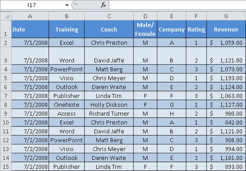
A training center has created a database to capture information about seminars conducted by the trainer. This data needs to be evaluated. The database has the dynamic name CourseInfo. The following database fields are available (see Figure 2-37):
Date
Training
Coach
Male/Female
Company
Rating
Revenue
The training center wants to know how many Excel seminars were conducted since it started to collect information. The DCOUNTA() function returns the result.
The DCOUNTA() function counts the number of cells in a column, list, or database that are not empty and that meet the specified conditions (see Figure 2-38).
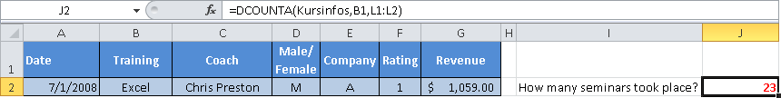
Define the criteria range for the filter. The criteria range consists of the column heading and the filter criterion in the cell below. To do this, copy the range B1:B2 into cells L1:L2. The formula =DCOUNTA(CourseInfo,B1,L1:L2) returns 23 Excel seminars.
You can find the number of other seminars by changing the filter in L2, for example, to Microsoft Word.
Next, the training center wants to know how much revenue the Excel seminars generated. You can use the DSUM() function to find this answer. This function adds the numbers in a column in a database that meet the specified conditions (Figure 2-39).
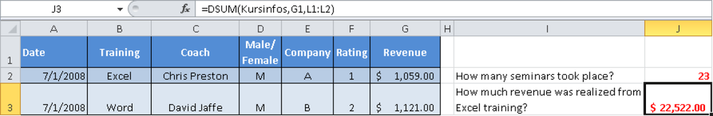
The formula =DSUM(CourseInfo,G1,L1:L2) returns a revenue of $ 22,522 generated from Excel seminars.
The training center is also interested in the average rating for the trainers and the seminars. You find this by using the DAVERAGE() function. This function provides the average of the ratings that meet the specified conditions (see Figure 2-40).
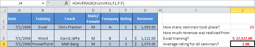
In this case, you don’t need the criteria range L1:L2, because no filter is required. The formula =DAVERAGE (CourseInfo,F1,F:F) returns an average rating of 1.88.