If you want to use the financial math functions of Excel, you will need to be familiar with their use. Excel can provide the calculations but not the interpretation. The Excel functions and the corresponding offline help aren’t a substitute for a relevant textbook.

There is a mistaken belief that the financial math functions of Excel are specially tailored to business and financial mathematics in the United States and have only partial relevance for other countries. Maybe this is the reason that the majority of financial math books steer clear of Excel. If Excel is integrated, it is typically used only as a pure spreadsheet program, and the functions are rarely used. This book is one of the few that explains all the financial math functions of Excel in detail and includes examples.

Financial mathematics spans several areas, including statistics and differential and integral calculus, but there are areas such as the evaluation of equity warrants and other derivative financial products that cannot be handled by Excel.

A simple interest calculation is characterized by the fact that the interest is not added to the capital at the due date. This kind of calculation is mostly used for short periods. A simple interest calculation is basically a simple percentage calculation. Financial mathematics offers many different interest terms.

In all cases, the interest is the price for borrowed (borrowing rate) or loaned (credit interest) capital. The interest rate relates to a certain period (often a year). Initially there are two different interest calculations: annuity and anticipative interest yield. Additional interest terms are nominal interest, real interest, and market interest. There are also terms that directly relate to interest: cash discount, bonus, rebate, markup, and markdown.

Annuity refers to a normal savings account or a common mortgage loan. The interest is calculated and paid at the end of the interest period for the initial capital. The anticipative interest yield is usually used to honor a bill, for federal funding, and for building loan contracts.

The interest is paid for the capital due at the end of the period and calculated based on the interest rate.

If a customer deposits money in his savings account in the middle of the year, calculating the interest at the end of the year is not difficult. If the money is in the account for four months and the interest rate is 3 percent, only a third of the interest per annum is paid. But this simple percentage calculation should take into account the correct days when determining the proportion of the year, and for this you can use the DAYS360() function. If a bill with a maturity of one month is presented and the bank sets an interest per annum of 6 percent, the bank keeps (without fees) 0.5 percent (a twelfth of the interest per annum) of the bill amount and pays the difference. To count the days, you could use the DAY360() function again. However, for this task Excel provides the PRICEDISC() function.

The table in Figure 2-46 outlines the step-by-step calculations. The number of days in the period is calculated in F2, and this is applied to the annual interest rate to determine the rate for the period. Applying this rate to the principal results in a value of $9,950. Excel provides the function PRICEDISC() to perform this calculation. This example makes it clear that functions simplify calculations but that the use of these functions requires some knowledge of their functionality.

Figure 2-46. Bill calculation as percentage calculation.

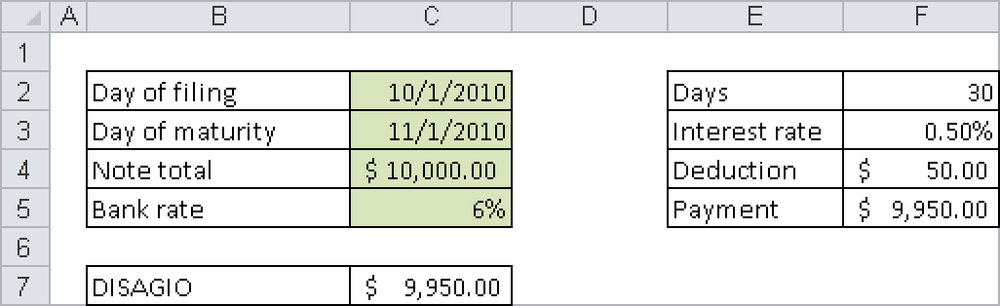
The example reveals something else: At what (annual) interest rate do you have to invest $9,950.00 to be paid $10,000.00 after one month, including interest? The answer is 50/9950*12=6.03 percent. This is also a simple percentage calculation. For this calculation, Excel offers the YIELDDISC() function. There is another function you can use: INTRATE(). You have to pass the data on the left in Figure 2-46 to this function to get the result.

In this example (for annuity), the interest to be paid is added to the initial capital and thus becomes part of the capital. This results in compound interest. This use of formulas requires the interest rate to remain the same over the entire period. This is not always realistic, but it is common in some investment models. If you invest $10,000 for 10 years, the bank might offer an interest rate of 4.8 percent. A detailed overview of this account is shown in Figure 2-47.

Figure 2-47. Progress of an account with an opening balance of $10,000.

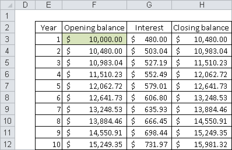
To calculate the result of $15,981.32, you don’t need any functions; you only have to add the interest to the capital at the end of the year.

Excel contains a function group that includes the FV() function. The name of this function is an acronym for future value, which is also called accumulated value. This function in the formula

=FV(4.8%,10,,-10000)

where $10,000 is invested for 10 years at an interest rate of 4.8 percent, returns $15,981.33. Why the difference? The deviation occurs because each amount entered as a deposit, withdrawal, or interest credit has to be rounded to two decimal figures (there are no smaller monetary units). This fact cannot be incorporated by the function in a math formula, because the math formula calculates to a high degree of accuracy. So you have to use the ROUND() function to round the amount at each stage. Limiting the cells to only two decimal figures is not sufficient and can lead to errors.

The calculation of compound interest serves as the basis for the examples in the remainder of this section.

An Annuity Calculation Example

An annuity is the periodic payment of the same amount. All functions available in Excel assume that the payment date for the annuity is the same as the interest date. The only differences are for annuities in advance and annuities in arrears, which are paid at the end of the period.

This example can be extended with the depositor adding another $2,000 to the account each year. The calculation of the account is shown in Figure 2-48.

Figure 2-48. Investment plus savings.

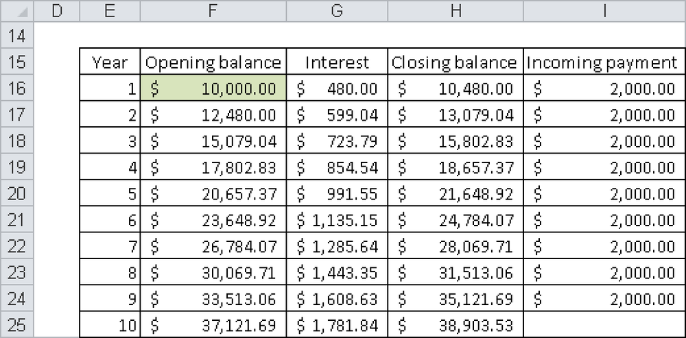
Here the FV() function is also useful:

=FV(4.8%,10,-2000,-10000)-2000  = 38903.52

$2,000 is invested each year for 10 years at an interest rate of 4.8 percent and added to the opening balance of $10,000. Because there is no deposit made on the last day, you have to subtract the last $2,000 from the payments calculated with FV(). In this calculation there is also a small rounding error.

Calculating Repayment

Financial mathematics uses three basic forms for the repayment of a loan—repayment through a single payment at the end (often in connection with life insurance), repayment through installments in consistent amounts (common for the purchase of merchandise), and repayment through annuity payments for which the repayment amount plus interest stays the same (the type of credit commonly used to finance real estate).

The last type is basically an annuity calculation, but the roles of the creditor and debtor are switched. The Excel function to calculate repayments covers only the first and the third types.

The formula used previously can also be used to calculate annuity repayments. In most cases, the annual interest rate has to be divided by 12 to calculate the monthly interest. The monthly interest is then used in the formula.

For example, assume that a bank offers the following financing for real estate: a $100,000 loan, at 5.6 percent per annum (p.a.) nominal interest (a five-year fixed rate), and 1 percent p.a. repayment. The bank also provides the following information:

• Monthly payment: $550.00

• Initial annual percentage rate: 5.75 percent

The monthly payment ensues from a twelfth of the interest rate of 5.6 percent plus a repayment of 1 percent: 6.6 percent/12 of the loan amount. The total is $550.00. With the following formula, you can calculate the effective rate:

=EFFECT(5.6%,12)

Figure 2-49 shows the repayment plan for the first year, which you can create without any special financial functions.

Figure 2-49. A repayment plan for an annuity loan.

This repayment plan shows that more than the agreed-upon one percent is repaid at the end of the year. This is caused by monthly payments during the year (the twelfth part). The effective rate has to be higher than the nominal interest because the agreed-upon amount had to be repaid faster. The Excel functions allow you to calculate single items, such as the interest of the fifth month, the principal balance at the end of the 16th month, or the annual percentage rate that usually cannot be calculated in a simple equation.

The order of the current quotation of prices isn’t based on divided durations but on parts of the year.

Investment Appraisal Example

Investments are often calculated with static or dynamic investment analyses. These might include cost/revenue comparisons as well as the payoff period and are based on cost and payment calculations. Dynamic methods consider the compound interest and evaluate deposits and withdrawals. These methods are not commonly used in commerce because of the models and the static collection of data. Excel provides several functions for dynamic investment calculations (capital value method and internal interest rate method). These methods are ideal for investment analyses.

For calculating the income returns, take the values shown in Figure 2-50 and enter them in a worksheet.

Figure 2-50. A simple example for a internal capital return.

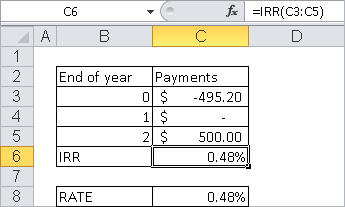
Here the IRR() function provides the fastest result, but you could also use the RATE() function or GOAL.SEEK.