
You’ve heard people refer to “applying mathematics to everyday life,” right? What exactly does that mean?
Even though you have learned a lot in school and during our professional training, you don’t always apply what you have learned to your observations in everyday life. This is especially true when it comes to mathematics and sciences. You have witnessed this many times.
However, sometimes it just happens. For example, consider a group of boys who are playing with a rope. Among them is Kevin, a boy who is a little younger and shorter than the others, but who is trying to make up for his deficiencies in years and height by being smarter.
Kevin and another boy are handling the rope, which the other boys are jumping. Kevin is now trying to take the rope away from the other boy. But this does not work. The other boy is too big and strong. As soon as the other boy is distracted, Kevin quickly and forcefully moves his hands up and immediately down again. The jerk moves along the rope and rips the rope out of the other boy’s hands.
How does the jerk arrive at the other boy’s end? Now let’s focus on the rope. Luckily Kevin tries to repeat his success, while on the other end the rope is being held tightly again. Another jerk, and then another, but this time his buddy is watching out. A double-jerk: You can clearly see how this jerking can cause several spikes upward and downward, running down the rope. The form of these spikes seems very familiar. Correct—they are sine curves. We are watching a mechanical model for the distribution of electromagnetic waves in an electrical conductor. If you would like to take another look at the sine curves, you can go back to Chapter 16 and read the description of the SIN() function.
Can Kevin show us more? Now our young protagonists are holding the rope still. There is nothing special happening—or is there more to it? Which shape does a hanging rope have? The answer to this question can also be found in Chapter 16, this time under COSH(). You can also look in the index under “catenary,” which is the name of this shape.
Now Kevin has tied one end of the rope to a jungle gym and moves the loose end up and down. Are those sine curves again? No. They get smaller toward the tied end, and the shape is different somehow. What Kevin is illustrating so nicely here is called damped oscillation. And how can these curves be described mathematically? “By using Bessel functions!” is the answer. These functions are explained in this section. However, you should first take a look at the diagrams for the BESSELJ() and BESSELY() functions (Figure 17-12 and Figure 17-16) in Figure 17-12 and Figure 17-16.
The Bessel functions (or cylindrical functions) are the solutions found during the integration of Bessel’s differential equation by series expansion. For certain electro-technical problems, they offer an exact (or at least close to exact) calculation, for example, for electric displacement in conductors. They are also used for describing vibrations and the associated damping; for calculating the orbits of planets and orbit abnormalities, for which they were introduced by Friedrich Wilhelm Bessel (an astronomer from Königsberg, Germany, 1784–1846); and for the simulation of pump tests in hydrogeology. They are also important in quantum mechanics, satellite geodesy (ground survey), and communication technology. They are usually generated as solutions for wave equations based on cylindrical boundary conditions.
In addition to the Bessel functions, there are two separate functions. These functions calculate the probability that a certain value is located within or outside of a Gauss distribution (see the description of NORMSDIST() in Chapter 12).
Syntax. BESSELI(x,n)
Definition. This function returns the modified Bessel function of the first kind, In(z), which corresponds to the Bessel function Jn evaluated for purely imaginary arguments.
Arguments
x (required) The value for which the function is to be evaluated; x must be a real number and can have values of ±700. (The value range varies with the order n.)
n (required) The order of the Bessel function, which must be positive and an integer. If n is not an integer, the decimal places are ignored; that is, n is truncated, not rounded.
Background. In(x), like Kn(x), belongs to the modified Bessel functions that increase or decrease exponentially—unlike the normal Bessel functions Jn(x) and Yn(x), which oscillate. In(x) is the solution of the slightly modified Bessel’s differential equation
x2y” + xy’ – (x2 + n2) · y = 0
or

This modified Bessel function of the first kind In(x) can be described as the loop integral
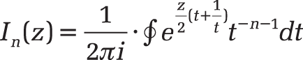
of the nth order. For a real number ν, the function can be calculated with
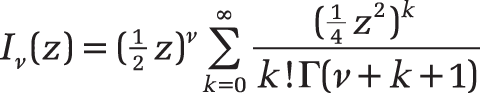
where Γ(y) is the gamma function.
Example. Using Bessel functions requires extensive knowledge of the application area. Therefore, this chapter will not use very specific practical examples. Instead, the example is explained through the mathematical properties and their graphical representation, as shown in Figure 17-9.
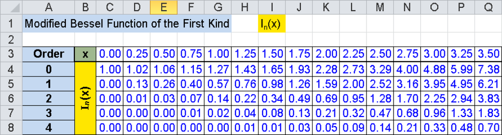
Figure 17-9. Excerpt from the Excel worksheet Bessel_I.xls for calculating the function values for the orders 0 to 4.
The cell with the text Order has the reference A3 in the sample file. C4 through Q8 contain the formulas with the BESSELI() functions. The first argument, the x value, is located in the cells above these formulas in row 3. Column A in the same row contains the second argument, the function order, which is the same for all formulas in a row. For example, the complete formula in C4 would be:
=BESSELI(C$3,$A4)
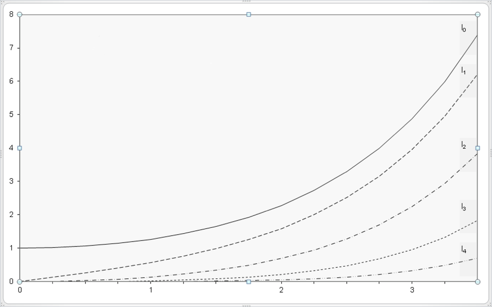
From the range C3 through Q8, the diagram in Figure 17-10 can be created, which graphically displays the modified Bessel function of the first kind. The exponential increase is easy to see. Even for small x values, it already generates high amounts.
Syntax. BESSELJ(x,n)
Definition. This function returns the Bessel function of the first kind, Jn(x).
Arguments
x (required) The value for which the function is to be evaluated; x must be a real number and can have values between –1.34·108 and +1.34·108. (The value range varies with the order n.)
n (required) The order of the Bessel function; must be positive. If n is not an integer, the decimal places are ignored, not rounded.
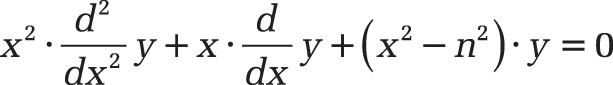
Background. The Bessel function of the first kind Jn(x) is the solution of Bessel’s differential equation
x2y” + xy’ + (x2 – n2) · y = 0
or
For a real number ν, the function can be calculated with
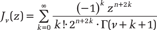
where Γ(y) is the gamma function.
Example. Because of the very special character of the Bessel functions, this book uses only their graphical representation, as with the other Bessel functions.
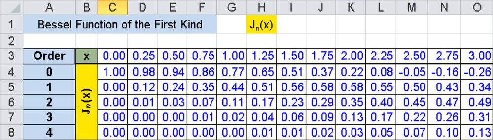
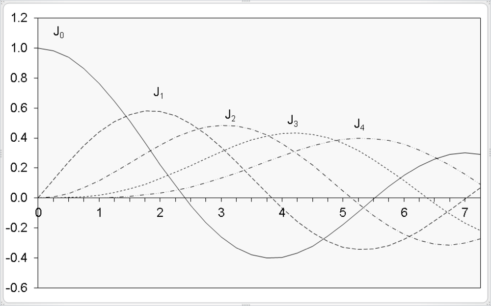
In the worksheet shown in Figure 17-11, which you can also find in the sample files, the function values for BESSELJ() are calculated with the orders 0 to 4 and displayed in a graph (see Figure 17-12).
Syntax. BESSELK(x,n)
Definition. This function returns the modified Bessel function of the second kind, Kn(x).
Arguments
x (required) The value for which the function is to be evaluated; x must be a real number and can have values of +1·10–307 to more than +700. The exact value of the upper limit of x depends on the order n (and the reverse is also true), but it is higher than any numbers used in practice.
n (required) The order of the Bessel function; must be positive and an integer larger than 100. In practice, however, there are only orders of less than 10. If n is not an integer, the decimal places are ignored; that is, n is truncated, not rounded.
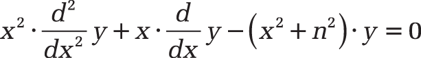
Background. Kn(x) corresponds to the Bessel functions Jn and Yn evaluated for purely imaginary arguments. Sometimes it is called the Basset function, the Macdonald function, or the modified Bessel function of the third kind. It is the solution to the modified Bessel’s differential equation
x2y” + xy’ – (x2 + n2) · y = 0
or
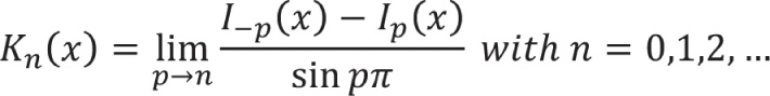
The modified Bessel function of the second kind, Kn(x) of the order n, can be expressed in terms of the modified Bessel function of the first kind, In(x):
Examples. Because of the very special character of the Bessel functions, this chapter uses only their graphical representation, as with the other Bessel functions.
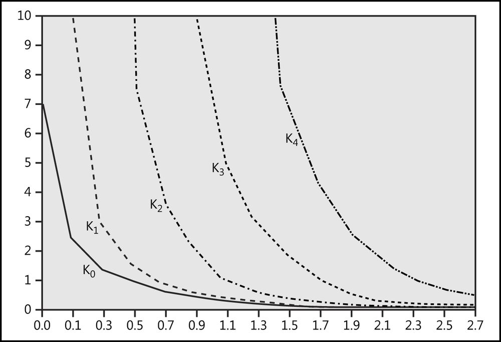
In the worksheet shown in Figure 17-13, the function values of the BESSELK() function for the orders n = 0...4 can be calculated and graphically displayed, as shown in Figure 17-14.
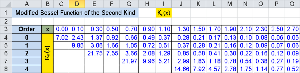
For the higher orders, the first formulas are omitted, because their function values are too large for a clear graphic.
Syntax. BESSELY(x,n)
Definition. This function returns the Bessel function of the second kind, Yn(x).
Arguments
x (required) The value for which the function is to be evaluated; x must be a real number larger than 0 and can have values up to 1.34·108. (The upper limiting value varies slightly with the order n.)
n (required) The order of the Bessel function; must be positive. The maximum value of n depends on x but covers all areas with practical relevance. If n is not an integer, the decimal places are ignored (not rounded).
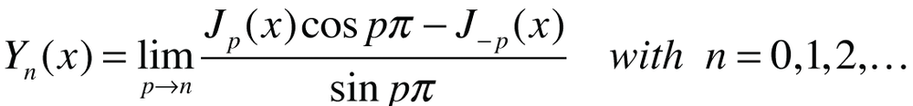
Background. The Bessel function of the second kind, Yn(x) of the order n, which is also called the Weber function or the Neumann function, is the solution of the Bessel’s differential equation
x2y” + xy’ – (x2 – n2) · y = 0
or

It can be expressed in terms of the Bessel function of the first kind, Jn(x):
Examples. Because of the very special character of the Bessel functions, this chapter uses only their graphical representation, as with the other Bessel functions.
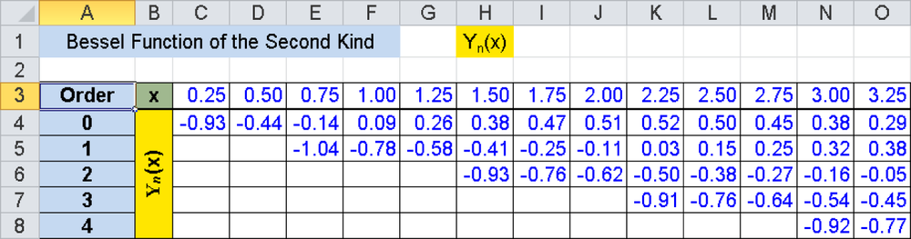
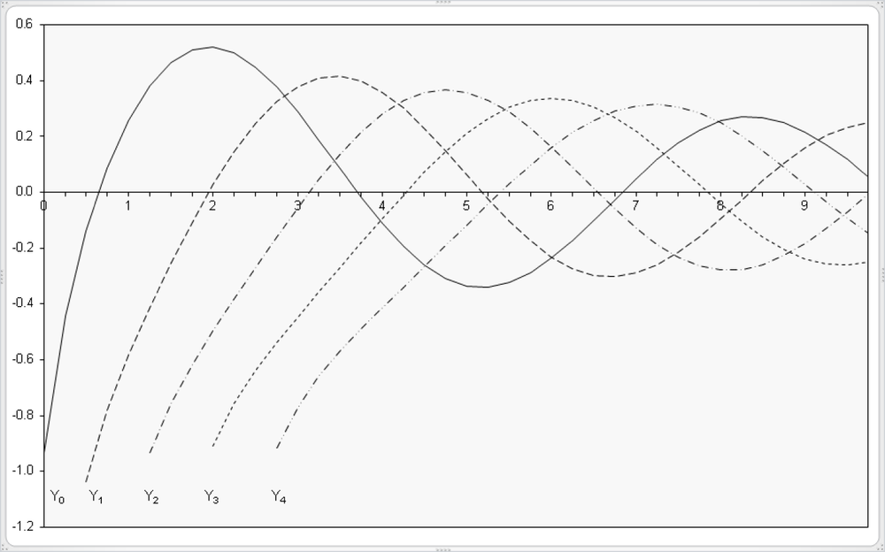
In the worksheet shown in Figure 17-15, the function values of the BESSELY() function for the orders n = 0...4 can be calculated and graphically displayed, as shown in Figure 17-16. For the higher orders, the first formulas are omitted, because their function values are too large for a clear graphic.
Syntax
ERF.PRECISE(Limit)
ERF(Lower_Limit,Upper_Limit)
Definition. These functions return the values of the probability integral (also called the Gauss error integral or the error function). For Excel 2010, the algorithm of the ERF() function has been improved. In addition, a similar function was introduced that does nearly the same thing but has a new name: ERF.PRECISE(), which can accept only one argument. This function calculates the error function in the range of 0 up to Limit. If Limit is negative, the lower limit is given by Limit, and the upper limit is set to 0. If you require backward compatibility, the earlier version of the function can be used without any disadvantages, and the following explanations apply as well.
Arguments
Lower_Limit (required) The lower limit for the integration into ERF().
Upper_Limit (optional) The upper limit for the integration into ERF(). If this argument is missing, ERF() integrates from zero to Lower_Limit.
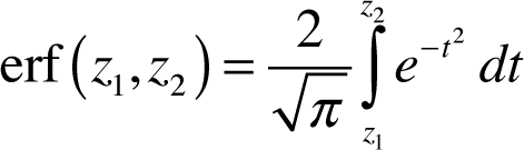
Background. The Gaussian error function erf(z) is returned by integrating the normal distribution of the normalized format of the Gauss function. It has the following format:
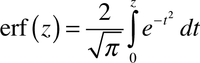
In the Excel function, the lower limit is also a variable and can be entered as the first argument to allow coverage of special cases. With the integration limits z1 and z2, the “generalized error function” erf(z1,z2) is defined as follows:
Examples. The following examples illustrate this function.
=ERF(0,0.5)returns0.520499878.=ERF(0.5)also returns0.520499878.=ERF(0.5,1)returns0.322200915.
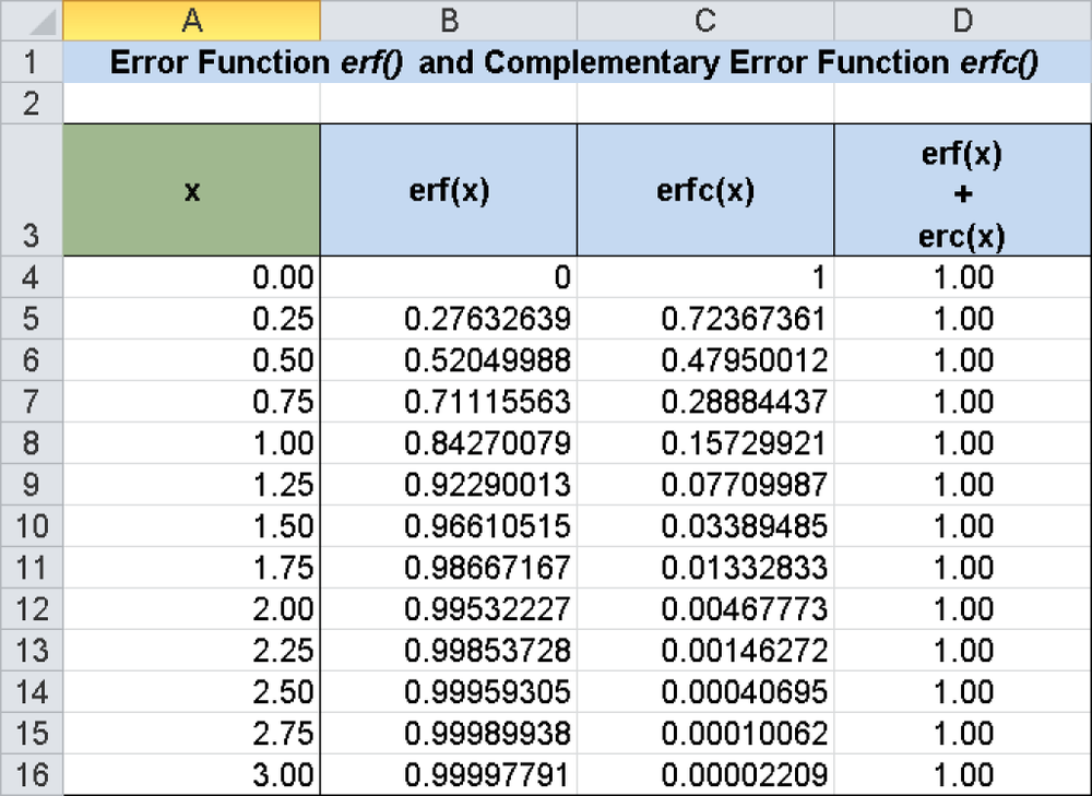
Figure 17-17 shows more examples of the function values of ERF() with the arguments Lower_Limit = 0 and Upper_Limit = 0...3. As a comparison, the function values of the ERFC() function in the same interval are listed next to it.
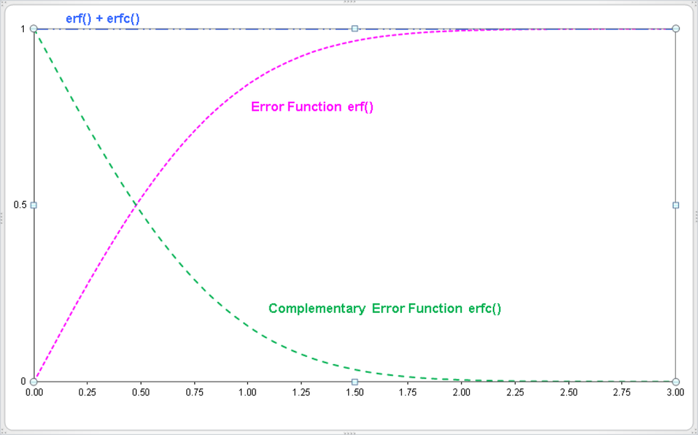
The diagram (Figure 17-18) graphically displays the connection between ERF() and ERC(): Both functions total a value of 1 at each location.
Syntax
ERFC.PRECISE(Lower_Limit)
ERFC(Lower_Limit)
Definition. These functions return the complement to the Gaussian error function in the range of Lower_Limit up to infinity. For Excel 2010, the algorithm of the ERFC() function has been improved. Now it can accept a negative argument. In addition, a similar function was introduced that does nearly the same thing, but it has a new name: ERFC.PRECISE(). If you require backward compatibility, the former version of the function can be used without any disadvantages, and the explanations here apply as well.
Argument
Lower_Limit (required) The lower limit for the integration into ERFC(). This function recognizes only one argument.
Background. The complement erfc(z) of the Gaussian error function erf(z) (see the Background section in the description of ERF() in Background) results from the following relationship:
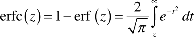
The upper integration limit is set to infinity (∞). ERFC(z) requires only one variable, z (the only argument, which consequently is also called Lower_Limit).
Example. See the examples section for ERF.PRECISE()/ERF() in Background for more examples for this function.