
Chapter at a glance
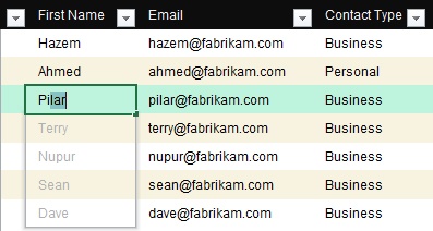
Flash Fill
Quickly extract text from adjacent data to fill a column, Identifying what’s new in Excel 2013

Analyze
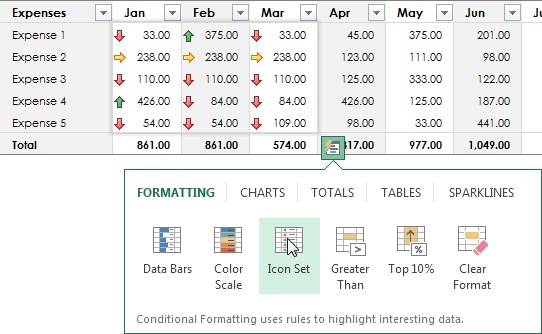
Use Quick Analysis tools to apply formats, add totals, and more, ???
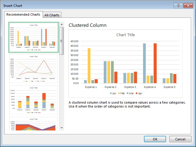
Chart
Let Excel provide recommendations based on selected data, ???
Filter
Use the Timeline feature to display data from a specific timeframe, ???

IN THIS CHAPTER, YOU WILL LEARN HOW TO
Start Excel 2013.
Identify what’s new in Excel.
Use the new features in Excel 2013.
Microsoft Excel 2013 is a spreadsheet application that allows you to organize, sort, calculate, and otherwise manipulate data by using formulas. Excel spreadsheets are organized into columns and rows but can also include other features, such as graphs and charts.
It doesn’t matter if your spreadsheet is simple or complex, because this part of the book provides you with the foundation for all of your needs. In this chapter, you’ll get familiar with the Excel 2013 user interface and using the ribbon. You will also get a glance at features that are new to this latest version of Excel.
You typically start Excel 2013 from the Windows Start screen in Windows 8 or the Start menu in Windows 7. You can also start Excel 2013 and open a file at the same time by opening a workbook from an email attachment, or by double-clicking a file on the desktop or in the File Explorer.
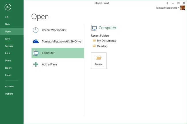
When you start Excel without opening an existing file, the new Start screen is displayed.
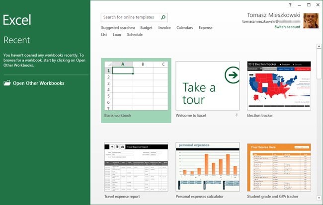
From the Start screen, you can open a recently used workbook, open an existing workbook, create a new workbook from a template, or just start with a fresh, blank workbook.
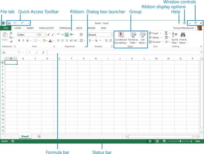
The following list describes some of the most important interface elements; places you’ll visit almost every time you employ Excel.
Ribbon. The main component of the Excel interface is where you’ll find the primary commands for working with the content of your workbooks. The ribbon contains task-oriented tabs; each tab contains groups of related commands. For example, on the Home tab, the Clipboard group contains commands for copying and pasting information in your workbooks. Command groups with additional commands not shown on the ribbon include a dialog box launcher button. Clicking the dialog box launcher displays a dialog box or a pane that contains related options. For example, if you click the dialog box launcher for the Font group, the Font dialog box appears, providing more formatting choices such as Strikethrough, Superscript, and Subscript.
Important
Your display settings may be different than those used for the graphics shown in this book. The ribbon may appear different on your screen due to its dynamic capabilities. For example, some buttons may appear stacked vertically without labels, or horizontally with labels.
See Also
For instructions on how to modify your display settings and adapt exercise instructions, see Chapter 1.
File tab. The first tab on the ribbon is unlike other ribbon tabs. Clicking the File tab does not display a ribbon tab; it instead displays the Backstage view, a place where you can find commands that apply to the entire workbook, such as Save As, Print, Share, and Export. The Backstage view is also where application options are located and where you can find information about your user account and your version of Office.
Quick Access Toolbar. Holds your most frequently used commands. By default, Save, Undo, and Redo have already been added.
Title bar. Appears at the top of the window and displays the name of the active workbook along with the application name. If your workbook hasn’t yet been saved, the title bar displays a name such as Book1 – Excel. After the workbook has been saved, the title bar will reflect the name of the saved workbook.
Window controls. Along with the standard Minimize, Restore Down/Maximize, and Close buttons available on the right side of the title bar, there are two additional buttons, the Help button and the Ribbon Display Options button, which is new in Excel 2013.
Status bar. Appears at the bottom of the window and displays information about the current workbook, such as the total and average of the values in the currently selected cells. On the right side of the status bar are view options for switching your workbook to a different view, along with a zoom slider to change the magnification of your active workbook.
See Also
For a more comprehensive list of ribbon and user-interface elements, along with detailed instructions on how to customize your user interface, including the ribbon and Quick Access Toolbar, see Chapter 1.
A lot of work went into the Windows 8 and Office underpinnings for this release of Excel. Microsoft also invested effort in producing some excellent, helpful new features, plus extensions and improvements of existing features.
Flash Fill. When you are entering data, Flash Fill uses predictive fills and offers to autocomplete the remaining pattern for you. Use Flash Fill to split a full name into first and last names, change the case of text, extract a name from an email address, and more.
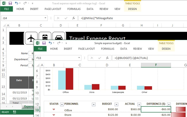
Separate workbook windows. Workbook windows no longer share the same user interface. Now you can display workbook windows on separate monitors and compare formulas between workbooks. Each workbook has its own ribbon that can be used independently of other open Excel windows.
Quick Analysis. Get applicable conditional formatting, charts, totals, tables, PivotTables, and in-cell charts, called sparklines, for a selected region of data. If you’re not sure about what to use, a live preview will help you visualize a suggestion prior to applying it.
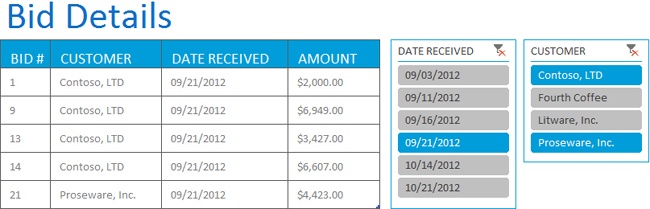
Table Slicers. These filter lists of information to your selected Slicer items. And, when your list is filtered, Table Slicers show you what you’ve selected along with other list data that’s relevant to your current filter.
Recommended Charts. If you know you need a chart, but aren’t sure about where to begin, the Recommend Charts feature will display the most relevant chart suggestions by using your selected data to help you determine which chart to use.
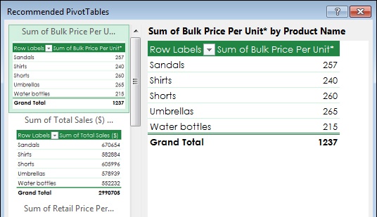
Recommended PivotTables. Get help summarizing and creating reports for your information. Instead of trying to determine a PivotTable layout prior to adding one, you can use the Recommended PivotTables feature, which will suggest various layouts based on your data that will assist you with creating a PivotTable.
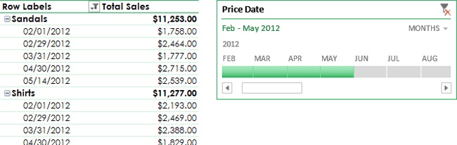
Timeline. When working with information that includes dates, you can add a timeline to filter your content to specific months or years.
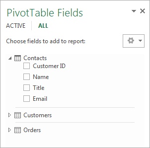
Multiple data sources in PivotTables. Instead of being limited to a single data table, you can relate tables with common information and add fields from those tables to your PivotTable report.


The following is a list of discussions in this book that explain how to use some of the new features in Excel 2013, with handy cross-references.
Flash Fill. See Introducing Flash Fill in Chapter 18.
Quick Analysis. See Using the Quick Analysis tools in Chapter 20.
Recommended PivotTables. See Creating a PivotTable in Chapter 20.
New Templates. See Exploring a built-in template in Chapter 20.
Recommended Charts and PivotCharts. See Creating and modifying a chart in Chapter 23.
Timeline. See Adding a timeline to a chart in Chapter 23.
The following are some other changes that you’ll notice in Excel 2013:
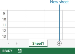
One sheet in a new workbook. There is now only one sheet in a new workbook, not three, as in previous versions of Excel. You add sheets by clicking the New Sheet plus-sign button (+).
Tip
Specifying the number of sheets in a new workbook is one of the many settings that you can change. For example, to construct a number of annual-summary-type workbooks, you might find it helpful to begin with 13 sheets; one for each month plus a summary sheet. To increase or decrease the default number of sheets that appear in new workbooks, change the Include This Many Sheets option on the General page of the Excel Options dialog box. You can specify up to 255 sheets.
See Also
For more information about working with multiple worksheets, see Creating a multisheet workbook in Chapter 22.
New functions. There are about 50 new functions in Excel 2013, most of which were added for increased compatibility with Open Document Format (ODF) 1.2, a universal royalty-free document format used by spreadsheet, chart, word-processing, and presentation applications, including StarOffice and OpenOffice.
New chart controls. Charts now have new dynamic floating controls—Chart Elements, Chart Styles, and Chart Filters—to make reworking an existing chart quicker and easier.
Rich chart data labels. You can now apply more formatting and graphic treatments to data labels in charts. You can even change the chart type, while preserving the label formatting.
Chart animation. When you change the underlying data for a chart, rather than changing immediately, the resulting change animates the chart as it changes to show the new values, which serves to emphasize the effects on the bigger picture.
Slicers. Slicers have a new interface in Excel 2013, which makes it easier to understand relationships. You can now use Slicers in data tables, not just in PivotTables.
PivotTable Field List. The new Field List includes fields from one table or multiple tables.
Standalone Pivot Charts. You can now detach a chart created by using PivotTable data, so that it can be repurposed elsewhere without its parent PivotTable.
Excel Data Model. Some of the functionality of the PowerPivot add-in is now built in as the Excel Data Model, allowing you to access multiple large data sources quickly and efficiently.
PowerView. Create presentation-quality reports by using graphics and data from multiple tables with the PowerView add-in, which uses data from the Excel Data Model exclusively.
Strict Open XML file format. For anyone who has experienced problems calculating data by using dates from 1900 or earlier, the Strict Open XML file format is compliant with the ISO8601 specification, solving leap-year and 2-digit-year problems.
The major interface elements of Excel 2013 are unchanged from 2010.
Most of the tools you need to do your work are located on the ribbon; if you need more tools, click a dialog-box launcher button to display a relevant dialog box with more options.
There are many new features in Excel 2013, which you will learn more about in the upcoming chapters.