
Chapter at a glance
Summarize
Use the AutoSum button to create quick totals and more, Using functions

Deduce
Create simple formulas by typing operators and clicking cells, Using functions
Calculate
Use built-in functions to create complex formulas, Using functions
Simplify
Use defined names to make formulas easier to read, Clean Up
IN THIS CHAPTER, YOU WILL LEARN HOW TO
Create, edit, and copy formulas.
Use functions.
Work with text in Excel.
Restrict cell entries.
There are some pretty flashy features in Microsoft Excel, more with every new release. This chapter has possibly the lowest flash quotient of any in this section, because we’re covering the basics of Excel—manipulating numbers. In other words, we’re talking more about adding, subtracting, multiplying, dividing, rounding, truncating, converting, extrapolating, square-rooting, and otherwise manipulating raw data to create information. It’s why Excel exists; it’s what Excel does best, and it’s all about what you need to know.
As a bonus, we’ll look at how to manipulate text. If you routinely process a lot of text-based data like inventory or address lists, and you combine first and last names into full names, Excel may become your favorite tool.
In this chapter, you’ll learn to use cell references and functions in formulas, give names to cells and ranges for easier referencing, and use formulas to edit text.
Practice Files
To complete the exercises in this chapter, you need the practice files contained in the Chapter19 practice file folder. For more information, see Download the practice files in this book’s Introduction.
Formulas are “backward” in Excel. In other words, we all learned in elementary school that 1+1=2 is how you write a formula. But in Excel, you flip the equal sign to the other side, so typing =1+1 into a cell returns the desired result. Putting the equal sign in front of the expression is the signal that tells Excel that you are entering a formula for which you want a calculated result. Anything else is just text, as far as calculations are concerned.
1+1= | This is a text entry in Excel. |
=1+1 | This is a formula in Excel. |
Tip
Though Excel also allows you to begin a formula with a plus or minus sign instead of an equal sign; after you press Enter, Excel adds a preceding equal sign anyway, and keeps the sign if it’s a minus.
So, you begin entering your formula with an equal sign, and then by using the correct language, including numbers (or constants), math operators, cell references, and functions, you can calculate just about anything from a shopping list to an Excel music video.
In this exercise, you will use the most common formula-editing features in Excel to create a simple formula and copy it to other cells.
Set Up
You need the Fabrikam-Seven-Year-Summary_start.xlsx workbook located in the Chapter19 practice file folder to complete this exercise. Open the Fabrikam-Seven-Year-Summary_start.xlsx workbook, and save it as Fabrikam-Seven-Year-Summary.xlsx.
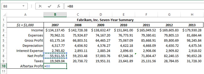
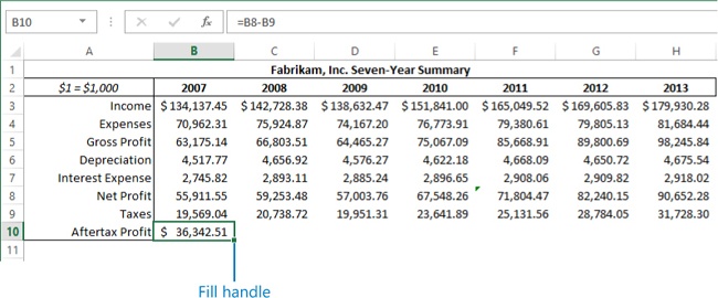
Open the Fabrikam-Seven-Year-Summary.xlsx workbook, and make sure that cell B10 is selected.
Enter = (an equal sign), then click cell B8 (containing the 2007 Net Profit figure), and you’ll notice several things: cell B10 remains selected, there is a dotted marquee around cell B8, and the cell reference =B8 appears in both cell B10 and the formula bar.
Enter – (a minus sign), and then click cell B9.
Press the Enter key, then press the Up Arrow key to reselect cell B10.
Although you could arrive at the same result by typing =55911.55-19569.04 into cell B10, a better way to leverage Excel’s talents is to use references to cells containing values that appear on the worksheet. This example formula should always produce a correct result, even if the numbers in cells B8 and B9 change. And sometimes the referenced cells contain other formulas, which is the case in this example (cell B8).
Click cell B8 and notice the formula =B5-B6-B7, which calculates net profit by subtracting depreciation and interest expense from gross profit.
Click cell B3 (2007 Income), enter 123456, and notice that cells B5, B8, B9, and B10 all change accordingly, because they are all dependent upon the value in cell B3, called a precedent cell.
Press Ctrl+Z to undo your last entry, and the dependent cells return to their previous values.
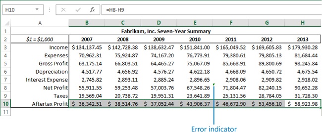
Select cell B10 and drag the fill handle across to column H to fill in the rest of the formulas.
Press Tab to inspect the formula in cell C10; repeat until you reach cell H10 and notice that the new formulas all reflect their relative locations. The cell references were adjusted by AutoFill. This is the easiest way to complete a row or column of identical formulas.
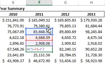
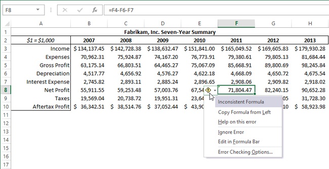
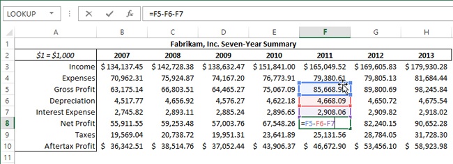
You’ll notice that there is a small triangle in the corner of cell F8. This is an indication that there is something different about this cell; that it somehow does not match the adjacent cells. It alerts you that there might be a problem with your formula.
Click cell F8 and an alert symbol will appear adjacent to the cell; click it to display the menu shown below.
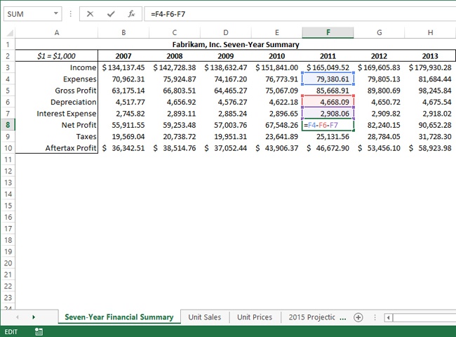
This menu offers possible solutions for the erring formula, and in this case, you could choose Copy Formula from Left, which would solve the problem. Instead, double-click cell F8 to enter Editing mode.
Notice that the word Edit appears in the lower-left corner of the Excel window, and that each cell referenced in the formula is highlighted.
This formula was entered incorrectly; subtracting depreciation and interest from cell F4, expenses, instead of cell F5, gross profit. You could simply highlight the reference in the formula and enter the correct reference, or you can manipulate the references directly. Whenever possible, it is always advisable to use direct manipulation with cell references in formulas, in order to minimize errors. Plus, it’s just easier to see the relationships among cells.
Point to the thick border of the box highlighting cell F4 and notice that it thickens just a bit when you pass over it.
Click the border and drag the box from cell F4 down to cell F5; the formula changes to reflect the newly highlighted cell.
Press Enter; the triangle indicator disappears, and the newly edited formula returns the correct net profit amount.
You can drag the formula-editing boxes anywhere on the sheet, or if you click one of the square dots in the corners, you can drag to expand the cell reference to include more rows and columns of cells.
You can create a lot of formulas by using math operators: addition, subtraction, multiplication (asterisk), division (forward slash), square root (caret), parentheses, and percentage symbols. But far more computational power is at your disposal with functions, which are essentially prepackaged formulas that perform specific calculations. All functions are followed by a set of parentheses, and most require specific arguments to be entered between them.
Although you can use cell references with math operators in simple formulas, you cannot use range references. But when you use functions, range references are perfectly acceptable to use as arguments, when appropriate.
The simplest and most-often-used function is SUM, which accommodates any number of arguments up to 255. For example, the following formulas all return totals:
=12+334
=C6+C7+C8
=SUM(C6:C8)
=SUM(12,334)
=SUM(12,334,C6:C8)
With most functions, you can combine different types of arguments, including single cell references, cell ranges (C6:C8), static values (12), and even other formulas. (Formulas within formulas are said to be nested.)
Tip
It is usually better to enter cell references in formulas, rather than entering static values, because you can see and change values entered into cells, but they are “hidden” in formulas; only the result of the formula is displayed. Keeping your numbers visible makes it easier to troubleshoot and audit worksheets.
You might expect that Excel would offer a quick and easy way to apply the most-often-used function in the galaxy, and you would be correct.
In this exercise, you will use the “epsilon” button, also known as the Sum button or AutoSum, for more than just totals.
Set Up
You need the Fabrikam-Seven-Year-Summary.xlsx workbook from the previous exercise to complete this exercise. Or, you can open the Fabrikam-Seven-Year-Summary_start.xlsx workbook located in the Chapter19 practice file folder and save it as Fabrikam-Seven-Year-Summary.xlsx.
Open the Fabrikam-Seven-Year-Summary.xlsx workbook, and click the Unit Sales worksheet tab.
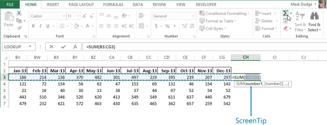
Click cell A3, then hold down the Ctrl key and press the Right Arrow key to jump to the rightmost end of the table. Cell CG3 should be selected.
Important
Rows in Excel are numbered 1 through 1,048,576 down the left side of the worksheet, but because there are only 26 letters in the alphabet, column letters are repeated. Column Z is followed by columns AA, AB, AC, and so on. After AZ comes BA; after ZZ comes AAA, and so on until you reach XFD, the 16,384th column.
Press the Right Arrow key once to select cell CH3.
Click the AutoSum button, located in the Editing group on the Home tab. (You can also hold down the Alt key and press = to enter a SUM function.)
Notice what just happened. After you clicked the AutoSum button, Excel inserted an equal sign, the function name, a set of parentheses, and the suggested argument, eliminating the need to type them. In this case, Excel correctly identified the range you want to sum. You can scroll back to the left to check this before you press Enter to lock in the formula. The AutoSum button sometimes gets it wrong, especially if the row or column label (for example, “FABK-0001” in cell A3) is a calculable numeric value such as a date, so you always need to check. You can also get help on the function before you press Enter.
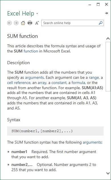
Click the SUM function name that is displayed in the ScreenTip floating just below cell CH3, and the Excel Help window appears, displaying information about the function.
Close the Help window by clicking the X in the upper-right corner.
Press Enter to finish the formula in cell CH3.
Click the tiny downward-pointing arrow to the right of the AutoSum button to display a menu of additional functions you can apply by using this button, in addition to SUM.
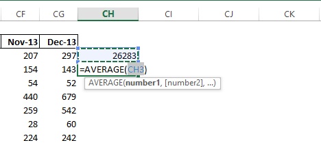
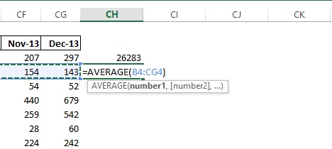
Click Average to enter the function on the worksheet; you’ll see that cell CH3 is the suggested argument to the AVERAGE function, which is definitely not what you want.
With the AVERAGE function still visible and the cell still in Edit mode, click cell CG4, just to the left of the new formula.
Hold down Ctrl and press the Left Arrow key to jump all the way to the left end of the table (cell A4), then release the Ctrl key and press the Right Arrow key to select cell B4 instead.
Hold down both the Shift and Ctrl keys, and then press the Right Arrow key to select cells B4:CG4.
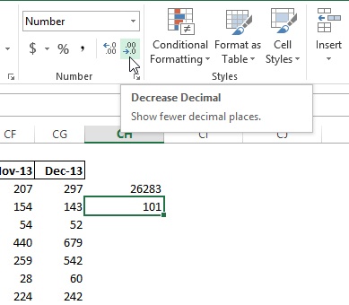
Press Enter, then press the Up Arrow key to reselect cell CH4 so you can see the formula, which now displays the average unit sales for this product, 100.8928571.
Decimal values in your averages are distracting, so to fix this, make sure that cell CH4 is still selected and click the Decrease Decimal button, located in the Number group on the Home tab, and keep clicking until the decimal portion of the number is hidden from view and until the rounded integer value 101 appears. (Remember that the actual value has not changed, only the displayed value.)
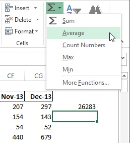
As you can see, when you click the menu arrow next to the AutoSum button, it offers other functions, including:
Count Numbers. Returns only the number of cells in the referenced area that contain numbers; cells containing text are ignored.
Max. Returns the maximum value in the referenced area.
Min. Returns the minimum value in the referenced area.
More Functions. Opens the Insert Function dialog box, where you can select any function. Contrary to what you might expect, this does not add the selected function to the AutoSum menu.
Using the status bar to check totals and more
The status bar is another handy feature you can use to quickly check the sum or average of any selected cells. Select some cells containing, well, anything, and then look at the bottom of the Excel window at the status bar. There you’ll see the Average, Count, and Sum. (Note that the default status bar readout for Count is a tally of cells with contents of any kind, not just cells containing numbers.) If you don’t need to create a formula, this is a real timesaver. You can modify the items displayed in the status bar by right-clicking the status bar to display the Customize Status Bar menu.
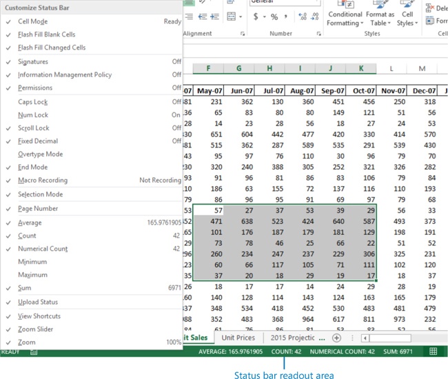
All items with check marks on the Customize Status Bar menu are currently active, even if there is no current corresponding item visible in the status bar. When, for example, you use Flash Fill, one of the two Flash Fill “mode” messages appears on the left side of the bar. Most of the menu items are mode indicators that appear only when appropriate. The last three—View Shortcuts, View Slider, and Zoom—turn the controls on the right end of the status bar on and off. You can add status bar readouts for Numerical Count, Minimum, and Maximum; to do so, click the corresponding menu item.
The SUM function is pretty easy to figure out, but there are hundreds of functions available, and most of them are not nearly as intuitive. Click the Insert Function button—the little fx button on the formula bar—to display the Insert Function dialog box, which comes in handy when you need to use functions with multiple arguments. Offering assistance in context, it explains the function and its possible variations, and makes it easy to enter even the most complex nested-formula arguments correctly. If you want more information and “live examples,” you can still access the Help system from the Insert Function dialog box by clicking the question mark in the title bar.
In this exercise, you’ll create a formula and work with the formula bar.
Set Up
You need the Loan_start.xlsx workbook located in the Chapter19 practice file folder to complete this exercise. Open the Loan_start.xlsx workbook, and save it as Loan.xlsx.
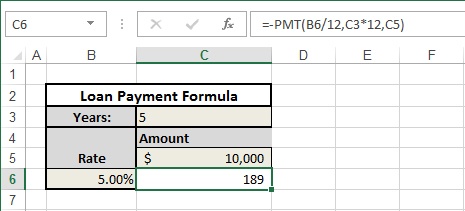
In the Loan.xlsx workbook, make sure that cell C6 is selected.
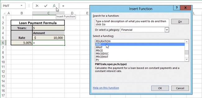
Click the Insert Function button in the formula bar, and notice that Excel inserts an equal sign (=) in the selected cell, in preparation for the formula that you are about to enter.
In the Or Select a Category list in the Insert Function dialog box, click the downward-pointing arrow and select Financial.
In the Select a Function box, scroll down the list and select PMT, which calculates the monthly payment on a simple loan; the syntax and description of the selected function appears below the function list.
Click OK to insert the function into the cell, which dismisses the Insert Function dialog box and displays the Function Arguments dialog box.
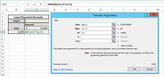
The first box in the Function Arguments dialog box—the Rate box—is active; click cell B6 (containing the percentage 5.00%) to insert that cell’s reference as the Rate argument. Notice that a short description of the selected argument appears in the bottom half of the dialog box. If you need more information, click the Help on This Function link at the bottom of the dialog box.
After the cell reference has been inserted, the cursor is still flashing in the Rate box; enter /12 to convert the rate from annual to monthly to create a nested formula within the PMT function; you can create up to 64 levels of nesting by using parentheses.
Click in the Nper box and then click cell C3 to insert the cell reference for the Years entry.
While the cursor is still in the Nper box, enter *12 to convert the time periods from years into months.
Click in the Pv box (present value), and then click cell C5; the loan amount is the present value.
As you add arguments in the Function Arguments dialog box, you’ll notice that Excel displays the actual calculated value of each argument to the right of each edit box, and shows the overall result that will be returned by the function, just below the argument values. If you watch cell C6 or the formula bar, you can keep an eye on the formula as it takes shape. Only the arguments that are displayed in bold in the dialog box are required; the Fv (future value) and Type arguments are optional.
Press OK to enter the formula.
This simple formula shows that your payments would be $189, but the result is displayed in parentheses as a negative number, because payments represent money spent rather than received. You might need to express cash outflows as negative values in a double-entry accounting worksheet, for example. However, if you don’t, it is common practice to reverse the sign for display purposes.
Select cell C6.
In the formula bar, click between the equal sign and the PMT function and enter – (a minus sign).
Press Enter.

You can explore the Insert Function dialog box to give yourself some perspective on the array of functions available and how they are organized.
There are three kinds of references in Excel: fixed, relative, and mixed. All of the cell references we have used thus far have been relative references, such as C4. Using relative references in formulas allows you to copy or fill the formula, and the relative references will adjust automatically. This is fine for many one-dimensional purposes like totals, as long as the data cells and the formula cells are always in the same relative positions.
For example, suppose in cell A1, you enter the formula =B1+C1. What this formula says, essentially, is “take the value in the next cell to the right, and add it to the value two cells to the right.” You can copy this formula anywhere, and the relative references will adjust automatically; the formula will always add the two cells to the right of the formula, wherever it is located.
But frequently, you might want to use a single value in multiple formulas, such as a percentage rate. You could use a relative cell reference, but only if you didn’t need to copy it elsewhere. Otherwise, you could use a fixed reference, such as $C$4. A dollar sign preceding the row number and column letter tells Excel to hold that position so it will not adjust when you copy it. You can use $C$4 in a formula, copying it as needed, and the cell reference will not change, because both the row and column are fixed.
You can also specify mixed references, in which one row or column is fixed and the other is relative; for example, $C4. When you copy this reference, the row adjusts automatically, but the column does not. You’ll use this ability to fix and mix your references in the next exercise.
In this exercise, you’ll change the reference style by using the F4 function key, which is a special unnamed reference-switching key that only works when you are editing formulas. This makes it easier and more reliable to edit formulas and requires a lot less squinting and typing the dollar signs yourself.
Set Up
You need the Loan_start.xlsx workbook from the previous exercise to complete this exercise. Or, you can open the Loan_start.xlsx workbook located in the Chapter19 practice file folder. Save the workbook as Loan.xlsx.
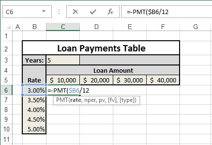
In the Loan.xlsx workbook, click the Loan Table worksheet tab.
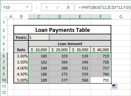
Make sure cell C6 is selected, and enter =-PMT( to begin the formula. (Make sure to include the minus sign after the equal sign.)
Click cell B6, which contains the 3.00% rate, to add the cell reference into the formula.
Press the F4 key and notice that the reference changes to the fixed form, $B$6.
Press F4 again, and it changes to B$6.
Press F4 a third time to change the reference to $B6, which is what you want; if you press F4 again, the reference returns to normal; you can keep pressing F4 to cycle through the sequence.
Following the reference $B6, enter /12 to convert the annual interest rate into a monthly amount.
Enter a comma to separate the first argument from the next, then click cell C3, which contains the number of years.
Press the F4 key just once this time, settling on the locked-row-and-column version of the mixed reference, $C$3.
Following the reference $C$3, enter *12 to convert years into months.
Enter a comma (,) and then click cell C5, which contains the $10,000 loan amount.
Press the F4 key twice this time to enter the locked-row version of the mixed reference, C$5.
Enter a closed parenthesis sign ()) to finish the function arguments.
Press Enter. Now you’re ready to copy the formula.
Tip
When you are in Edit mode and are working on a formula with multiple cell references, click the one you want to fix or mix; pressing F4 adjusts that reference only. And yes, you could just type the dollar signs yourself, but F4 actually does make it easier if you’re working with more than one reference.
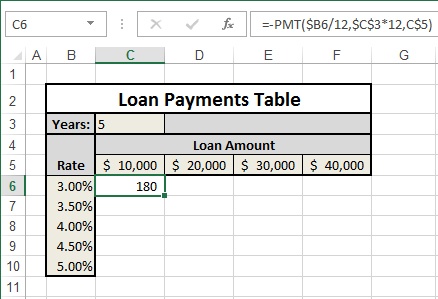
Select cell C6 and drag the fill handle to the right to cell F6.
Drag the fill handle from cell F6 down to cell F10.
Press Shift+Tab to highlight cell F10. (You can press Tab to move the selected cell to the right or down in a selected block of cells without losing the selection; pressing Shift+Tab moves the selection in reverse.)
In all of the copied formulas, the fixed reference $C$3 stayed locked on the Years cell, and the mixed references performed as expected, adjusting to use the correct rate in column B, and the proper loan amount in row 5. Filling in formulas even in a table this small would have been an unduly tedious and error-prone endeavor, had we entered each formula manually. Spending a little time crafting the formula made the table easier to create and rendered the results more reliable.
Another way to construct formulas is to use named ranges instead of cell references. Applying familiar names to cells and ranges makes them easier to remember.
In this exercise, you’ll create names to apply to cell references and ranges.
Set Up
You need the Fabrikam-Seven-Year-Summary2_start.xlsx workbook located in the Chapter19 practice file folder to complete this exercise. Open the Fabrikam-Seven-Year-Summary2_start.xlsx workbook, and save it as Fabrikam-Seven-Year-Summary2.xlsx.
Open the Fabrikam-Seven-Year-Summary2.xlsx workbook.
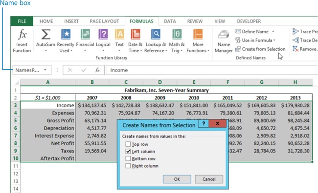
Click the tiny arrow in the Name box on the left end of the formula bar, and select NamesRange from the list to select the range A3:H10.
On the Formulas tab, click Create From Selection in the Defined Names group.
Select the Left Column check box, if it is not already selected, and then click OK.
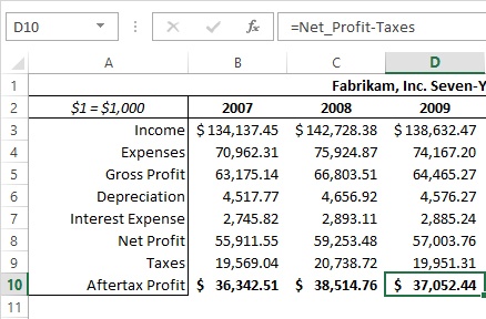
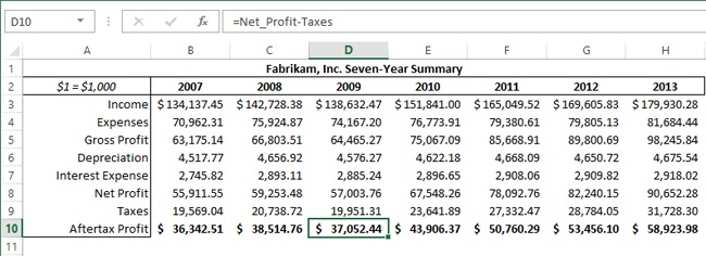
Select cell B10.
Enter =Net_Profit-Taxes and press Enter.
Select cell B10 again and drag the fill handle to cell H10 to copy the formula.
These formulas all create the same totals as the ones that you created in the first exercise in this chapter, except that now all the formulas in row 10 are exactly the same. This illustrates one of Excel’s hidden features, implicit intersection. The names Net_Profit and Taxes each represent a range of cells, not a single cell, but Excel correctly assumed that you wanted to use only the cell in each range that appears in the same column as the formula.
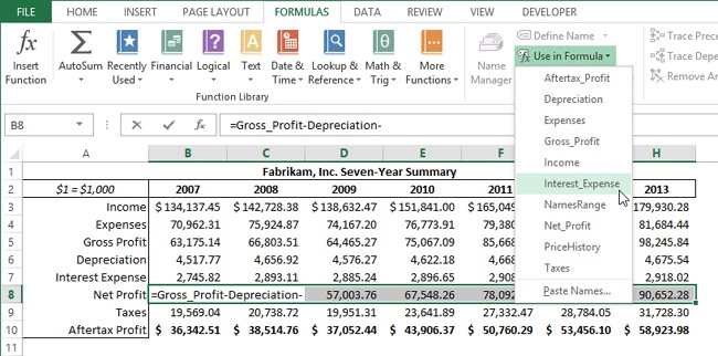
Select the Net Profit formulas in cells B8:H8.
Enter = (an equal sign), then click the Use in Formula menu in the Defined Names group.
Select Gross_Profit from the list of names, and then enter – (a minus sign).
Select Depreciation from the Use in Formula menu, and then enter – (a minus sign).
Select Interest_Expense from the list.
Press Ctrl+Enter to insert the formula into all the selected cells at once.
There is one more row of formulas you can edit yourself. Just perform the last four steps of this procedure on row 5 instead of row 8, and create the formula =Income-Expenses.
The categories listed in the Insert Function dialog box represent all functions, including very specialized functions that are used for such things as programming, engineering, and querying databases. There are frequently used functions in every category, of course, but for most of us, some categories will never have representatives in our favorites list. Viewing the Formulas tab on the ribbon reveals the types of functions available.
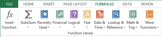
Next to giant versions of the Insert Function and AutoSum buttons (everyone’s favorites), the Function Library reveals the categories that we all use most; less frequently used functions are relegated to the More Functions menu. The Recently Used menu collects your own personal favorites.
Tip
When you have an idea of what you’re looking for, the Formulas tab may be more beneficial to you than the available choices in the Insert Function dialog box. When you select a function from the Function Library group, you skip the Insert Function dialog box and go directly to the Function Arguments dialog box.
In this section, we’ll focus on some helpful functions from the six categories represented on the Formulas tab, and you’ll be provided with brief explanations of each category. We encourage you to use the Excel Help system to enhance your understanding. You can access the Help system at any time by pressing F1 on your keyboard or clicking the Help button on the ribbon. You can also directly access a specific Help topic by clicking the More Help On This Function link at the bottom of the Insert Function dialog box.
In the Help topics, you’ll find descriptions and definitions, and most function topics will include live examples that you can download and test for yourself.
The following eight math and trig functions can be accessed through the AutoSum button:
SUMIF(range, criteria, sum_range). This command combines the IF and SUM functions to add specific values in a range according to the criterion you supply. For example, the formula =SUMIF(G5:G12, “X”, J5:J12) returns the total of all numbers in J5:J12, in which the cell in the same row in column G contains an X.
COUNTIF(range, criteria). This command is similar to SUMIF, but counts cells in the specified range that match your specified criterion.
SUMPRODUCT(array1, [array2], [array3], ...). This function multiplies each value in array1 by the corresponding value in array2, array3, and so on, then adds the totals. All the arrays (up to 255) must consist of an identical shape and size.
PRODUCT(number1, [number2], ...). This function multiplies all of its arguments (up to 255). If you need to multiply a lot of numbers, using this function is easier than creating a formula such as =A1+A2+A3+A4.
RANDBETWEEN(bottom, top). This function generates a random integer that falls between two provided integer values, inclusive. It is also volatile, meaning that it recalculates every time you open or edit a worksheet or press F9 (recalculate).
ROUND(number, num_digits). You can round a number by using this function for a specified number of digits. When num_digits is zero, number is rounded to an integer value; if num_digits is greater than zero, number is rounded to the specified number of decimal places; if num_digits is less than zero, the number is rounded to the indicated number of places to the left of the decimal point.
ROUNDDOWN(number, num_digits). Similar to ROUND, this function always rounds a number down, toward zero.
ROUNDUP(number, num_digits). Also similar to ROUND, this function rounds a number up, away from zero.
You can use logical functions to create complex conditional formulas, such as those mentioned in the following list:
IF(logical_test, [value_if_true], [value_if_false]). This function applies a logical test (for example, C5>200) that results in a true or false and optionally allows you to specify different values for both True and False results.
Nested IF. This function creates a hierarchy of tests. For example, the formula: =IF(A1=1, “Yes”, IF(AND(A1>=1, A1<10), “Maybe”, IF(AND(A1>=10, A1<20), “No”, “N/A”))) returns Yes if the value is 1, Maybe for values of 2 through 9, No for values between 10 and 20, and N/A if none of these conditions is true.
AND(logical1, logical2, ...). This function returns FALSE if any of its arguments are false, and returns TRUE only if all of its arguments are true. Generally, this function is used as an argument to another function, such as IF, which allows you to apply multiple logical tests instead of just one. Conversely, the OR function returns FALSE only if all of its arguments are false, and returns TRUE if any of its arguments are true. Either function can accept up to 255 arguments.
IFERROR(value, value_if_error). This function returns a specified value (or a message enclosed in quotation marks, such as “We have a problem!”) if the value argument evaluates to FALSE. You can use this function to test the results of other formulas by nesting them within the IFERROR function as the value argument.
Many functions can manipulate text. Some of them are pretty esoteric; for example, the BAHTTEXT function coverts any number into text in the Thai language.
Following are a few of the more useful text functions, shown with their arguments.
CLEAN(text). Removes all nonprintable characters. This is useful when you are importing data from other sources, which sometimes includes errant code symbols, returns, or line-break characters.
CONCATENATE(text1, text2, ...). See Combining text from multiple cells into one string later in this chapter.
EXACT(text1, text2). This function compares two text strings to see if they are the same. The function returns TRUE if they are exactly the same; otherwise, it returns FALSE. It is case-sensitive, but not formatting-sensitive.
LEFT(text, num_characters). This function returns the first num_characters in a text string. For example, the formula =LEFT(“Step by Step”,4) returns Step. Note that text entered directly into a formula must be enclosed in quotation marks. This tells Excel that you have entered a text string; the quotation marks don’t count as characters. If you use references to text in other cells; no quotation marks are needed. If cell C3 contained the text Step by Step, the formula =LEFT(C3,4) would also return Step.
LEN(text). Returns the number of characters in a text string. For example, the formula =LEN(“Step by Step”) returns a value of 12.
LOWER(text). Converts text into all-lowercase characters.
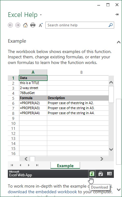
PROPER(text). See Changing the case of text later in this chapter.
RIGHT(text, num_characters). Returns the last num_characters in a text string. For example, the formula =RIGHT(“Step by Step”,7) returns the text by Step. Yes, spaces count as characters.
TRIM(text). See Removing extra spaces, later in this chapter.
UPPER(text). Converts text into all-uppercase characters.
You can use dates in formulas and functions as you would any other value. If cell A1 contains the date 7/4/2013, the formula =A1+300 returns the date that falls exactly 300 days later: 4/30/2014 (or the serial date value 41759).
To find the elapsed number of weeks between two dates, you can enter a formula such as =((“12/13/14”)-(“11/12/13”))/7, which returns 56.6 weeks. If you enter dates “in format,” then enclose them in quotation marks. Or you can use serial date values. But it’s always better to use cell references instead of entering any values into formulas directly, simplifying the previous formula to something like =(C4-D4)/7.
Following are several functions that do things that formulas cannot accomplish:
TODAY(). Inserts the current date. This function takes no arguments, but you must include the empty parentheses anyway. You may also need to apply a date format, if the date appears as an integer. This function is said to be volatile, meaning that it recalculates every time you open or edit the worksheet.
NOW(). Similar to the TODAY function, but it inserts both the current date and time. This function is also volatile and takes no arguments. The result includes an integer (the date) and a decimal value (the time).
WEEKDAY(serial_number, return_type). Returns the day of the week for a specific date. The serial_number can be a date value, a cell reference, or text such as “1/27/11” or “January 27, 2011” (you need to include the quotation marks). The function returns a number that represents the day of the week on which the specified date falls, where day 1 is Sunday if the optional return_type argument is 1 or omitted. If return_type is 2, then day 1 is Monday, if return_type is 3, then Monday is day 0, and Sunday is day 6.
WORKDAY(start_date, days, holidays). Returns a date for a specified number of working days before or after a given date. If the days argument is negative, the function returns the number of workdays before the start date; if days is positive, then it returns the number of working days after the start date. Optionally, you can include an array or range of other dates you wish to exclude as the holidays argument.
NETWORKDAYS(start_date, end_date, holidays). This function is similar to the WORKDAY function but calculates the number of working days between two given dates. This function does not count weekends.
These two lookup functions are designed to search for the largest value (either numerically or alphabetically) in a specified row or column of a table that is less than or equal to the lookup value, not for an exact match. The functions return errors if all the values in the first row or column of the table are greater than the lookup value, but if all the values are less than the lookup value, the function returns the largest value available.
VLOOKUP(lookup_value, table_array, col_index_num, [range_lookup]). Searches the first column of table_array and returns a value from the same row, in the column indicated by col_index_num. The values can be numbers or text, but it is essential that table_array is sorted in ascending order, top to bottom. No lookup_value should appear more than once in a table. This function returns the largest value that does not exceed lookup_value, not necessarily an exact match, unless you set the optional range_lookup argument to FALSE.
HLOOKUP(lookup_value, table_array, row_index_num, [range_lookup]). Searches the first row of table_array and returns a value from the same column, in the row indicated by row_index_num. Otherwise, this function performs identically to the VLOOKUP function, except that table_array must be sorted in ascending order from left to right rather than top to bottom.
ROW([reference]). Returns the row number of the reference; if the reference argument is omitted, returns the current row.
ROWS(array). Returns the number of rows in the specified range.
COLUMN([reference]). Returns the column number (not the letter) of the reference; if the reference argument is omitted, returns the current column.
COLUMNS(array). Returns the number of columns in the specified range.
Most of the financial functions involve various aspects of amortizing or annuitizing. There are clusters of functions that address such specifics as T-bills, mortgages, loans, and depreciation.
The following lists some of the most commonly used financial functions:
PMT(rate, number of periods, present value, future value, type). Computes the payment required to amortize a loan over a specified number of periods. For an example, see Using relative, fixed, and mixed cell references, earlier in this chapter.
IPMT(rate, period, number of periods, present value, future value, type). Computes the interest portion of an individual loan payment, assuming a constant payment and interest rate. PPMT takes the same arguments as IPMT but returns the principal portion of the payment.
NPER(rate, payment, present value, future value, type). Computes the number of periods required to amortize a loan, given a specified payment.
SLN(cost, salvage, life). Calculates straight-line depreciation for an asset.
People always think numbers when they think about Excel, but in reality, Excel is frequently used as a layout grid for text. Most of the time, this sort of thing would be better accomplished with Microsoft Word, but people use what they know and are comfortable with. However, there are some things you can do with text in Excel that you can’t do in Word. After learning a few more tricks, you may think about massaging text in Excel first, before copying it into a Word document.
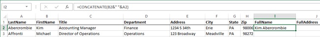
In this exercise, you’ll put strings of text together any way you want by using the CONCATENATE function. Whenever you use a cell reference in the function, you use the ampersand (&) as a connector to the next item, which can be another cell reference, or text enclosed in quotation marks. Anything you enter between the quotation marks is treated as text.
Set Up
You need the Fabrikam-Management2_start.xlsx workbook located in the Chapter19 practice file folder to complete this exercise. Open the Fabrikam-Management2_start.xlsx workbook, and save it as Fabrikam-Management2.xlsx.
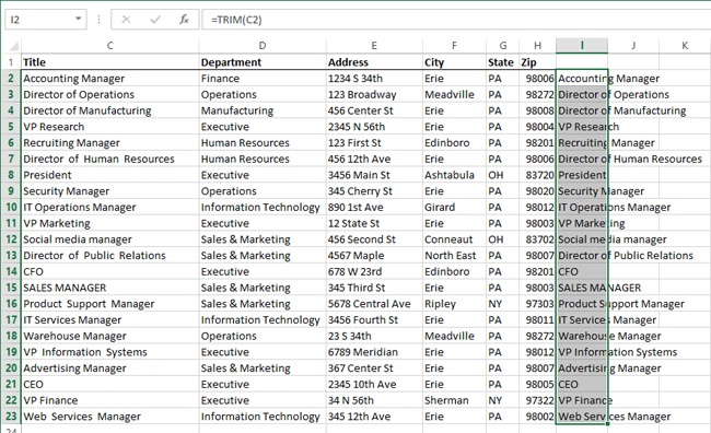
In the Fabrikam-Management2.xlsx workbook, make sure that cell I2 is selected.
Begin entering =CON.
A suggested list of functions appears below the cell.
Double-click CONCATENATE.
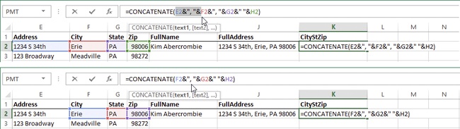
Click cell B2 and then enter &” “& (a space enclosed with quotation marks and ampersands).
Click cell A2 and press Enter.
Press the Up Arrow key, reselecting cell I2 to view the formula.
Select cell J2.
Enter =CON and double-click CONCATENATE.
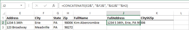
Click cell E2 and enter &”, “& (a comma and a space enclosed with ampersands and quotation marks).
Click cell F2 and enter &”, “&
Click cell G2 and enter &” “&
Click cell H2 and press Enter.
Double-click the border next to the Column letter J to auto-fit the contents.
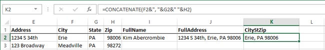
Double-click cell J2 to activate Edit mode.
In the formula bar, drag through the entire formula you just created and press Ctrl+C to copy it.
Press Esc to leave Edit mode.
Click cell K2 and press Ctrl+V to paste the formula. Notice that the cell references did not adjust. When you copy a formula using Edit mode, you can paste it into a new cell and the references are preserved.
Double-click cell K2 to activate Edit mode.
Drag to select the first part of the formula in parentheses E2&”, “& and press the Delete key. Notice that the formula argument selection box disappears from cell E2.
Press Enter.
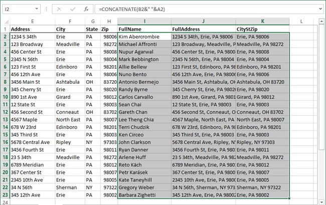
Select cells I2 to K2, then drag the fill handle down to row 23 to copy the relative-reference formulas.

If you were to concatenate cell references with only ampersands, the concatenated contents of the cells may not be separated by spaces, which is why we added them. You can also concatenate cells containing formulas; only the displayed results are included, not the formulas themselves. Thus, you could use a formula like the following to create a sentence that changes depending on the formula’s result:
=CONCATENATE("Sales for the month came in at "&E5&"!!")Assuming that cell E5 contains a monthly sales formula; this would result in a displayed value such as:
Sales for the month came in at $67,890!!
It’s inevitable that extra spaces will appear, especially in a document containing a lot of text that was entered by hand at some point in its history. In the previous exercise, for example, you might create or propagate double spaces when combining the contents of other cells. Fortunately, there’s a function in Excel to remove extra spaces.
In this exercise, you’ll remove extra spaces using formulas, and then you’ll copy and paste the results—only the displayed values from those formulas—to replace the spaced-out text.
Set Up
You need the Fabrikam-Management2.xlsx workbook from the previous exercise to complete this exercise. Or, you can open the Fabrikam-Management2_start.xlsx workbook, located in the Chapter19 practice file folder, and save it as Fabrikam-Management2.xlsx.
In the Fabrikam-Management2.xlsx file, make sure that Sheet2 is selected and that the cell range I2:I23 is selected.
Some entries in column C have extra spaces in them; for example, C7.
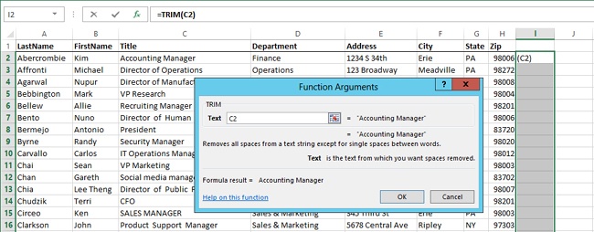
Click the Insert Function button in the formula bar.
Click the Or Select a Category list and click Text.
Scroll down through the list of Text functions and double-click Trim.
Click cell C2 to enter the cell reference into the Text box.
Press the Ctrl key and click the OK button; if you press Ctrl when entering any formula, Excel not only inserts the formula into the active cell, it also inserts it into all the selected cells.
Now, the cells that previously contained extra spaces have the spaces removed due to the use of the TRIM function (specifically, rows 7, 13, 16, 19, and 23).
The previous exercise used formulas to create a clean set of titles in column I, but now how do you get them back into column C? If you copy cells I2:I23 and simply paste them into column C, you get errors, because what you actually copied were formulas.
In this exercise, you’ll copy only the formulas’ results into column C.
Set Up
You need the Fabrikam-Management2.xlsx workbook from the previous exercise to complete this exercise.
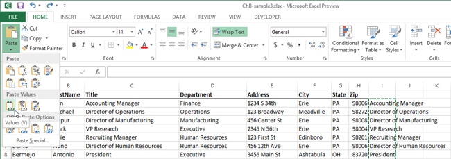
Make sure that Sheet2 is selected and that the range I2:I23 is selected, and then press Ctrl+C to copy it.
Click cell C2.
Click the menu arrow below the Paste button on the Home tab of the ribbon to display the Paste Options palette.
Click the Values button in the Paste Values group to replace the Titles in column C with the newly trimmed titles from your formulas.
Click the heading in column I to select the entire column.
Click the Clear button in the Editing group on the Home tab of the ribbon, and then click Clear Contents.
Case is another issue that comes up frequently when working with large amounts of text. You might have some text in caps and some in all lowercase, for example. Excel provides the tools you need to make the text formatting consistent.
In this exercise, you’ll change the case of text entries.
Set Up
You need the Fabrikam-Management2.xlsx workbook from the previous exercise to complete this exercise. Or, you can open the Fabrikam-Management2_start.xlsx workbook, located in the Chapter19 practice file folder, and save it as Fabrikam-Management2.xlsx.
In the Fabrikam-Management2.xlsx workbook, make sure Sheet2 is selected.
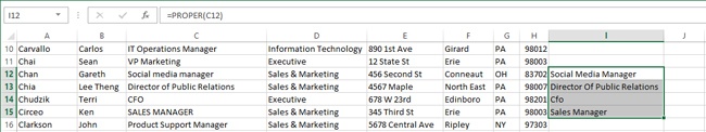
Click cell I12 and then click the Insert Function button in the formula bar.
Select the Text category, then scroll down through the function list, click PROPER, and then click OK.
Click cell C12 to enter its reference in the Text box, and then press Enter.
Select cell C12 and drag the fill handle down to cell C15 to copy the formula.
The Proper function did its job, but at the same time, it created other issues. The four text values in column I are now in proper case, meaning that the first letter of every word is capitalized. This is what you wanted in cells I12 and I15. However, the text in cells I13 (“Of”) and I14 (“Cfo”) contain some incorrect capitalization, but they serve to illustrate the function’s effect. We’ll copy only the ones we want and paste them, but this time we’ll use the right mouse button to display a shortcut menu.
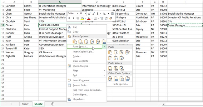
Click cell I12 and press Ctrl+C to copy.
Click cell C12, then click the right mouse button. Select Paste Special, and then click the Values button.
Click cell I15 and press Ctrl+C to copy.
Click cell C15, then click the right mouse button, select Paste Special, and then click the Values button.
Select cells I12 to I15 and press the Delete key to delete the formulas.
Wouldn’t it be nice if there were ways to prevent people (ourselves included) from entering the wrong type of data in critical cells? For example, let’s say you have a workbook that several people use to enter collected sales data every month—sales totals, inventory, and contact information—in dollars, integers, and text. A stray text character entered into a cell used in calculations could result in error values popping up all over the workbook. Worse yet, sometimes entry errors produce no visible errors, just bogus results. Excel addresses these concerns and offers Data Validation features to enhance the integrity of your data.
In this exercise, you’ll restrict cell entries to protect your data.
Set Up
You need the Real-Estate-Transition_start.xlsx workbook located in the Chapter19 practice file folder to complete this exercise. Open the Real-Estate-Transition_start.xlsx workbook, and save it as Real-Estate-Transition.xlsx.
In the Real-Estate-Transition.xlsx workbook, make sure that cell B2 is selected.
Enter any letter into cell B2 and press Enter.
Notice that many #VALUE! errors suddenly appear.
Press Ctrl+Z to undo the last entry.
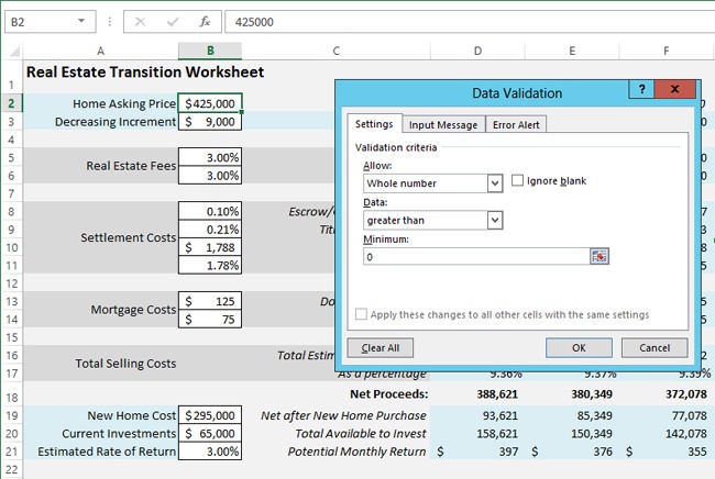
With cell B2 selected, click the Data tab on the ribbon and click the Data Validation button in the Data Tools group.
In the Data Validation dialog box, select Whole number in the Allow list.
In the Data box, select greater than.
Enter 0 (zero) into the Minimum box.
Click OK.
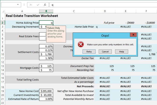
Enter any letter into cell B3 and press Enter.
Notice that Excel will not allow text to be entered into this cell, and an error message is displayed when you try to enter text into the cell.
Click Cancel.
Click the Data Validation button again.
Click the Input Message tab.
In the Title box, enter Values Only.
In the Input Message box, enter this text: Enter the asking price for your existing home.
Click the Error Alert tab.
In the Title box, enter Oops!
In the Error Message box, enter Make sure you enter only numbers in this cell.
Click OK.
Enter any letter into cell B3, and press Enter.
Now, any time you try to make an invalid entry into cell B3, a customized error message appears.
In the Oops! dialog box, press Cancel.
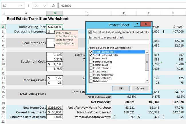
Click the Home tab.
Click the Format button in the Cells group, and then click Protect Sheet to display the Protect Sheet dialog box.
Click OK in the Protect Sheet dialog box.
Press Tab, and continue pressing Tab; you’ll notice that only the white cells with borders are selected.
The last two steps show what happens when you protect a sheet with specific cells unlocked. In the original practice file for this exercise, the bordered cells were unlocked, but the sheet wasn’t protected. By definition, all cells are “locked” in a new workbook, which actually means that the “locked format” has been applied. You can see this by clicking the Format button on the Home tab and looking at the Lock Cell command near the bottom of the menu. If the icon next to the Lock Cell command has a box around it, then the cell is locked; if not, it is unlocked. But this has no effect on anything until you click the Protect Sheet command (located above the Lock Cell command). When you click the Protect Sheet command, the Protect Sheet dialog box is displayed, offering editing options that allow changes to be made in unlocked cells when the sheet is protected. And, as shown in Step 24, when a sheet is locked, pressing the Tab key will always move the selection to the next unlocked cell; locked cells are ignored.
Click the Home tab on the ribbon, then click the Format button in the Cells group, and click Unprotect Sheet.
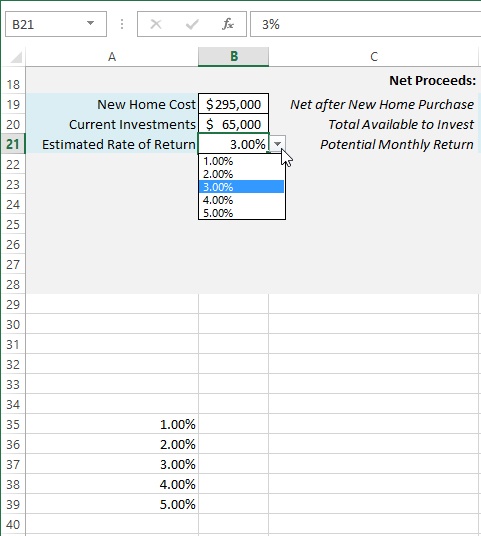
Select cell B21 (Estimated Rate of Return).
Click the Data tab, click Data Validation, and in the Allow list on the Settings tab, select List.
Click in the Source box and enter =rates.
Click OK.
Click the Home tab, then click the Format button in the Cells group, and click Protect Sheet.
Now, when you reselect cell B21, a small menu arrow appears alongside it, offering a number of different interest rates. Cells A35:A39 contain this list of options (the range is named rates). We could have entered the formula =$A$35:$A$39 into the Data Validation dialog box, but the name is not only easier to enter, it also makes it easier to edit. If you move or add more items to the list, just select the new list and redefine the name.
The Data Validation and Lock Cells features allow you to build bulletproof worksheets and maintain control of available options for specific data points. These features are beneficial when creating workbooks that will be used by new Excel users.
All formulas in Excel begin with an equal sign.
Double-click an existing formula to change cell references directly by dragging.
Excel automatically adjusts relative references in formulas when you copy or fill the cells containing them.
Adding a dollar sign before either the row number or column letter in a cell reference makes it a mixed reference, fixing that position and allowing the other to change automatically when copied.
Adding dollar signs before both the row number and column letter in a cell reference makes it a fixed reference, allowing you to copy the formula anywhere; it will always refer to the same cell.
If you double-click a cell containing a formula (putting it into Edit mode), you can copy the formula in the cell and paste it into another cell while preserving the references, whether they are mixed, fixed, or relative.
Using the AutoSum button is the easiest way to enter formulas to compute totals and averages, find the maximum or minimum value, and more.
The Insert Function dialog box provides a helpful user interface when you are using functions in formulas, and it provides information about the function, along with descriptive text and assistance for entering arguments.
You can use the CONCATENATE function to combine separate strings of text into one.
You can use the PROPER function to capitalize the first letter of every word in a text string.
When you copy cells containing formulas, you can use the Paste Special Values button to paste only their displayed values.
You can restrict cell entries to accept only numbers, dates, times, text, and more.
All cells are locked by default; when you protect a worksheet, only the unlocked cells are available for editing.