
Day 13 UTube
The Plan
Thanks to the recent advancements in the so-called chip-on-glass (COG) technology and the mass adoption of LCD displays in cell phones and many consumer applications, small displays with integrated controllers are becoming more and more common and inexpensive. The integrated controller takes care of the image buffering and performs simple text and graphics commands for us, offloading our applications from the hard work of maintaining the display. But what about those cases when we want to have full control of the screen to produce animations and or simply bypass any limitation of the integrated controller?
In today’s exploration we will consider techniques to interface directly to a TV screen or, for that matter, any display that can accept a standard composite video signal. It will be a good excuse to use new features of several peripheral modules of the PIC32 and review new programming techniques. Our first project objective will be to get a nice dark screen (a well-synchronized video frame), but we will soon see to fill it up with several useful and (why not?) entertaining graphical applications.
Preparation
In addition to the usual software tools, including the MPLAB® IDE, the MPLAB C32 compiler, and the MPLAB SIM simulator, this lesson will require the use of the Explorer 16 demonstration board and In-Circuit Debugger of your choice). You will also need a soldering iron and a few components at hand to expand the board capabilities using the prototyping area or a small expansion board. You can check on the companion Web site (www.exploringPIC32.com) for the availability of expansion boards that will help you with the experiments.
The Exploration
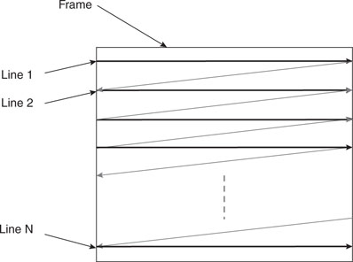
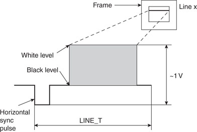
There are many different formats and standards in use in the world of video today, but perhaps the oldest and most common one is the so called “composite” video format. This is what was originally used by the very first TV sets to appear in the consumer market. Today it represents the minimum common denominator of every video display, whether a modern high-definition flat-screen TV of the latest generation, a DVD player, or a VHS tape recorder. All video devices are based on the same basic concept, that is, the image is “painted,” one line at a time, starting from the top left corner of the screen and moving horizontally to the right edge, then quickly jumping back to the left edge at a lower position and painting a second line, and so on and on in a zigzag motion until the entire screen has been scanned. Then the process repeats and the entire image is refreshed fast enough for our eyes to be tricked into believing that the entire image is present at the same time, and if there is motion, that it is fluid and continuous (see Figure 13.1).
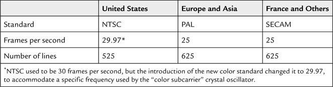
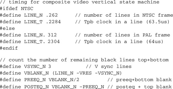
In different parts of the world, slightly incompatible systems have been developed over the years, but the basic mechanism remains the same. What changes is the number of lines composing the image, the refreshing frequency, and the way the color information is encoded.
Table 13.1 illustrates three of the most commonly used video standards adopted in the United States, Europe, and Asia. All those standards encode the “luminance” information (that is, the underlying black-and-white image) together with synchronization information in a similarly defined composite signal. Figure 13.2 shows the NTSC composite signal in detail.
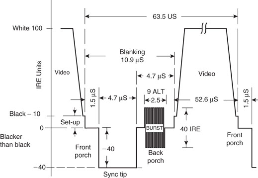
The term composite is used to describe the fact that this video signal is used to combine and transmit in one three different pieces of information: the actual luminance signal and both horizontal and vertical synchronization information.
The horizontal line signal is in fact composed of:
The color information is transmitted separately, modulated on a high-frequency subcarrier. A short burst of pulses in the middle of the back porch is used to help synchronize with the subcarrier. The three main standards differ significantly in the way they encode the color information but, if we focus on a black-and-white display, we can ignore most of the differences and remove the color subcarrier burst altogether.
All these standard systems utilize a technique called interlacing to provide a (relatively) high-resolution output while requiring a reduced bandwidth. In practice only half the number of lines is transmitted and painted on the screen in each frame. Alternate framespresent only the odd or the even lines composing the picture so that the entire image content is effectively updated at the nominal rate (25 Hz and 30 Hz, respectively). The actual frame rates are effectively double. This is effective for typical TV broadcasting but can produce an annoying flicker when text and especially horizontal lines are displayed, as is often the case in computer monitor applications.
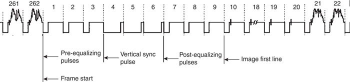
For this reason, all modern computer displays are not using interlaced but instead use progressive scanning. Most modern TV sets, especially those using LCD and plasma technologies, perform a deinterlacingof the received broadcast image. In our project we will avoid interlacing as well, but we’ll sacrifice half the image resolution in favor of a more stable and readable display output. In other words, we will transmit frames of 262 lines (for NTSC) at the double rate of 60 frames per second. Readers who have easier access to PAL or SECAM TV sets/monitors will find it relatively easy to modify the project for a 312-line resolution with a refresh rate of 50 frames per second. A complete video frame signal is represented in Figure 13.3.
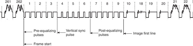
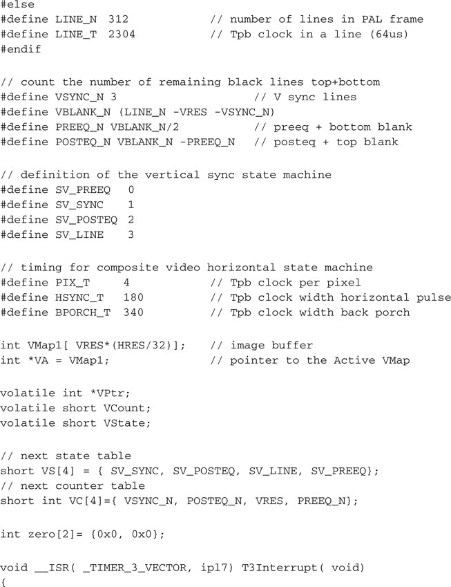
Notice that, of the total number of lines composing each frame, three line periods are filled by prolonged synchronization pulsesto provide the vertical synchronization information, identifying the beginning of each new frame. They are preceded and followed by groups of three additional lines, referred to as the pre- and post-equalization lines.
Generating the Composite Video Signal
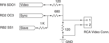
If we limit the scope of the project to generating a simple black-and-white image (no gray shades, no color) and a noninterlaced image as well, we can considerably simplify our project’s hardware and software requirements. In particular, the hardware interface can be reduced to just three resistors of appropriate value connected to two digital I/O pins. One of the I/O pins will generate the synchronization pulses and the other I/O pin will produce the actual luminance signal (see Figure 13.4).
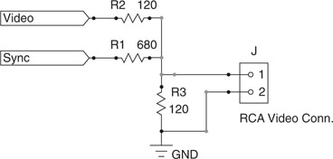
The values of the three resistors must be selected so that the relative amplitudes of the luminance and synchronization signals are close to the standard specifications, the signal total amplitude is close to 1 V peak to peak, and the output impedance of the circuit is approximately 75 ohms. With the standard resistor values shown in the previous figure, we can satisfy such requirements and generate the three basic signal levels required to produce a black-and-white image (see Table 13.2 and Figure 13.5).
Table 13.2 Generating luminance and synchronization pulses.
| Signal Feature | Sync | Video |
| Synch pulse | 0 | 0 |
| Black level | 1 | 0 |
| White level | 1 | 1 |
Since we are not going to utilize the interlacing feature, we can also simplify the pre-equalization, vertical synchronization, and post-equalization pulses by producing a single horizontal synchronization pulse per each period, as illustrated in Figure 13.6
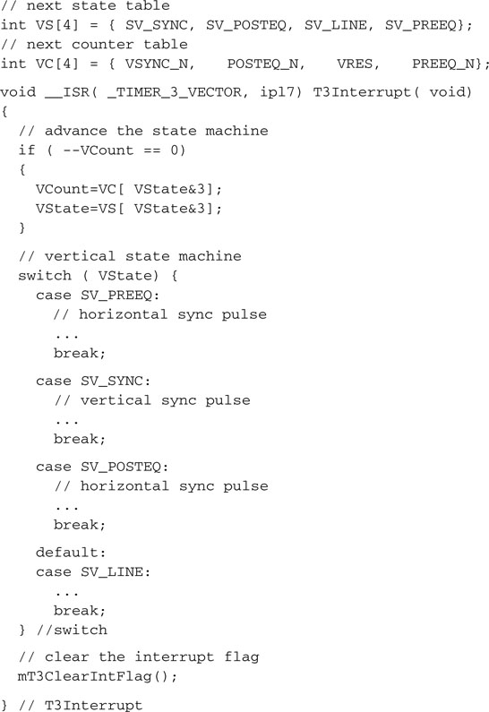
The problem of generating a complete video output signal can now be reduced to (once more) a simple state machine that can be driven by a fixed period time base produced by a single timer interrupt. The state machine will be quite trivial because each state will be associated with one type of line composing the frame, and it will repeat for a fixed amount of times before transitioning to the next state (see Figure 13.7).
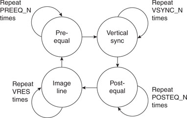
A simple table will help describe the transitions from each state (see Table 13.3).
Table 13.3 Video state machine transitions table.
| State | Repeat | Transition to |
| Pre-equal | PREEQ_N times | Vertical Sync |
| Vertical Sync | 3 times | Post-equal |
| Post-equal | POSTEQ_N times | Image line |
| Image line | VRES times | Pre-equal |
Although the number of vertical synchronization lines is fixed and prescribed by the video standard of choice (NTSC, PAL, and so on), the number of lines effectively composing the image inside each frame is up to us to define (within limits, of course). In fact, although in theory we could use all the lines available to display the largest possible amount of data on the screen, we will have to consider some practical limitations, in particular the amount of RAM we are willing to allocate to store the video image inside the PIC32 microcontroller (see Figure 13.8). These limitations will dictate a specific number of lines (VRES) to be used for the image, whereas all the remaining lines (up to the standard line count) will be left blank.
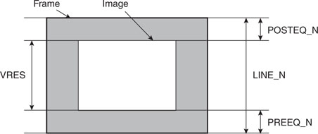
In practice, if LINE_N is the total number of lines composing a video frame and VRES is the desired vertical resolution, we will determine a value for PREEQ_N and POSTEQ_N as follows:
If we choose Timer3 to generate our time base, set to match the horizontal synchronization pulse period (LINE_T) as shown in Figure 13.5, we can use the timer’s associated interrupt service routine to execute the vertical state machine. Here is a skeleton of the interrupt service routine on top of which we can start flashing the complete composite video logic:
To generate the actual horizontal synch pulse output, there are several options we can explore:
The first solution is probably the simplest to code but has the clear disadvantage of keeping the processor constantly tied in endless loops, preventing it from performing any useful work while the video signal is being generated.
The second solution is clearly more efficient, and by now we have ample experience in using timers and their interrupt service routines to execute small state machines.
The third solution involves the use of a new peripheral we have not yet explored and deserves a little more attention.
The Output Compare Modules
The PIC32MX family of microcontrollers offers a set of five Output Compare peripheral modules that can be used for a variety of applications, including single pulse generation, continuous pulse generation, and pulse width modulation (PWM). Each module can be associated to one of two 16-bit timers (Timer2 or Timer3) or a 32-bit timer (obtained by combining Timer2 and Timer3) and has one output pin that can be configured to toggle and produce rising or falling edges as necessary (see Figure 13.9). Most importantly, each module has an associated and independent interrupt vector.
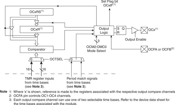
The basic configuration of the Output Compare modules is performed by the OCxCON register where a small number of control bits, in a layout that we have grown familiar with, allow us to choose the desired mode of operation (see Figure 13.10).
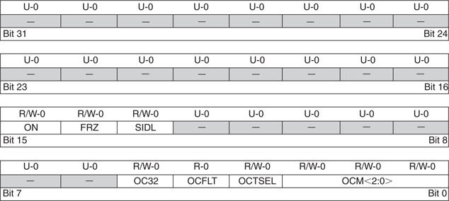
When used in continuous pulse mode (OCM=101) in particular, the OCxR register is used to determine the instant (relative to the value of the associated timer) when the output pin will be set, while the OCxRS register determines when the output pin will be cleared (see Figure 13.11).
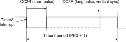
Choosing the OC3 module, we can now connect the associated output pin RD2 directly as our Synch output, shown in Figure 13.4.
We can also start flashing the vertical state machine body to make sure that in each state the OC3 produces pulses of the correct width. In fact, though during normal, pre-equalization, and post-equalization lines, the horizontal synch pulse is short (approx. 5us), during the three lines devoted to the vertical synchronization the pulse must be widened to cover most of the line period (see lines 4, 5 and 6 in Figure 13.6):
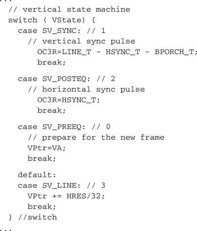
Image Buffers
So far we have been working on the generation of the synchronization signals Synch connected to our simple hardware interface (refer back to Figure 13.4). The actual image represented on the screen will be produced by mixing in a second digital signal. Toggling the Video pin, we can alternate segments of the line that will be painted in white (1) or black (0 ). Since the NTSC standard specifies a maximum luminance signal bandwidth of about 4.2 MHz (PAL has very similar constraints) and the space between front and back porch is 52us wide, it follows that the maximum number of alternate segments (cycles) of black and white we can display is 218, (52 × 4.2), or in other words, our maximum theoretical horizontal resolution is 436 pixels per line (assuming the screen is completely used from side to side). The maximum vertical resolution is given by the total number of lines composing each frame minus the minimum number of equalization (6) and vertical synchronization (3) lines. (This gives 253 lines for the NTSC standard.)
If we were to generate the largest possible image, it would be composed of an array of 253 × 436 pixels, or 110,308 pixels. If 1 bit is used to represent each pixel, a complete frame image would require us to allocate an array of 13.5 K bytes, using up almost 50 percent of the total amount of RAM available on the PIC32MX360. In practice, though it is nice to be able to generate a high-resolution output, we need to make sure that the image will fit in the available RAM, possibly leaving enough space for an application to run comfortably along and allowing for adequate room for stack and variables. There are an almost infinite number of possible combinations of the horizontal and vertical resolution values that will give an acceptable memory size, but there are two considerations that we will use to pick the perfect numbers:
Choosing a horizontal resolution of 256 pixels (HRES) and a vertical resolution of 200 lines (VRES) we obtain an image memory requirement of 6,400 bytes (256 × 200/8), representing roughly 20 percent of the total amount of RAM available. Using the MPLAB C32 compiler, we can easily allocate a single array of integers (grouping 32 pixels at a time in each word) to contain the entire image memory map:
![]()
Serialization, DMA, and Synchronization
If each image line is represented in memory in the VMap array by a row of (eight) integers, we will need to serially output each bit (pixel) in a timely fashion in the short amount of time (52us) between the back and the front porch part of the composite video waveform. In other words, we will need to set or clear the chosen video output pin with a new pixel value every 200 ns or faster. This would translate into about 14 instruction cycles between pixels, way too fast for a simple shift loop, even if we plan on coding it directly in assembly. Worse, even assuming we managed to squeeze the loop so tight, we would end up using an enormous percentage of the processing power for the video generation, leaving very few processor cycles for the main application.
Fortunately, we already know one peripheral of the PIC32 that can help us efficiently serialize the image data: It’s the SPI synchronous serial communication module. In a previous chapter we used the SPI2 module to communicate with a serial EEPROM device. In that chapter we noted how the SPI module is in fact composed of a simple shift register that can be clocked by an external clock signal (when in slave mode) or by an internal clock (when in master mode). Today we can use the SPI1 module as a master connecting the SDO (serial data output, RF8) pin directly to the Video pin of the video hardware interface, leaving the SDI (data input) and SCK (clock output) pins unused. Among the many new and advanced features of the PIC32 SPI module and the PIC32 in general there are two that fit our video application particularly well:
Operating in 32-bit mode, we can practically quadruple the transfer speed of data between the image memory map and the SPI module. By leveraging the connection with the DMA controller, we can completely offload the microcontroller core from any activity involving the serialization of the video data.
The bad news is that the DMA controller of the PIC32 is an extremely powerful and complex module that requires as many as 20 separate control registers for its configuration. But the good news is that all this power can be easily managed by an equally powerful and well-documented library, dma.h, which is easily included as part of plib.h.
The DMA module shares the 32-bit-wide system bus of the PIC32 and operates at the full system clock frequency. It can perform data transfers of any size to and from any of the peripherals of the PIC32 and any of the memory blocks. It can generate its own set of specific interrupts and can multitask, so to speak, since each one of its four channels can operate at the same time (interleaving access to the bus) or sequentially (channels activity can be chained so that the completion of a transfer initiates another). See Figure 13.12.
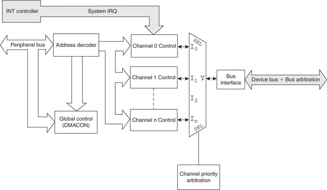
The arbitration for the use of the system bus is provided by the BMX module (which we have encountered before) and happens seamlessly. In particular, when the microcontroller cache system is enabled and the pre-fetch cache is active, the effect on the performance of the microcontroller can hardly be noticed. In fact, when an application requires a fast data transfer, nothing beats the performance and efficiency of the DMA controller.
The DMA module initialization requires just a couple of function calls:
So, for example, we can initialize channel 0 of the DMA controller to respond to the SPI1 module requests (interrupt on transmit buffer empty), transferring 32 bits (4 bytes) at a time for a total of 32 bytes per line, with the following three lines of code:
All we need to do is have the PIC32 initiate the first SPI transfer, writing the first 32-bit word of data to the SPI1 module data buffer (SPI1BUF), and the rest will be taken care of automatically by the DMA module to complete the rest of the line.
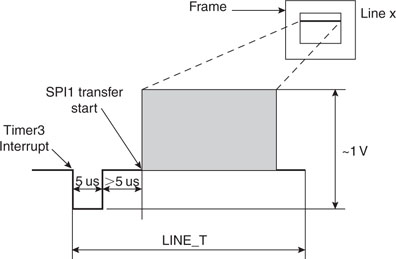
Unfortunately, this creates a new efficiency problem. Between the Timer3 interrupt marking the beginning of a new line period, and the beginning of the SPI1 transfer, there is a difference of about 10us. Not only this is an incredibly long time to “wait out” for a microcontroller operating at 72 Mhz (up to 720 useful instructions could be executed in that time), but the timing of this delay must be extremely accurate. Even a discrepancy of a single clock cycle would be amplified by the video synchronization circuitry of the TV and would result in a visible “indentation” of the line. Worse, if the discrepancy were not absolutely deterministic, as it could/would be if the PIC32 cache were enabled (the cache behavior is by its very definition unpredictable), this would result in a noticeable oscillation of the left edge of the screen. Since we are not willing to sacrifice such a key element of the PIC32 performance, we need to find another way to close the gap while maintaining absolute synchronization between horizontal synch pulse and SPI data serialization transfer start (see Figure 13.13).
By looking more carefully at the SPI module and comparing it with previous PIC® architectures, you will discover that there is one particular new feature that seems to have been added exactly for this purpose. It is called the Framed Slave mode and it is enabled by the FRMEN bit in the SPIxCON register. Not to be confused with the bus master and slave mode of operation of the SPI port, there are in fact two new framed modes of operation for the SPI. In framed mode, the SS pin, otherwise used to select a specific peripheral on the SPI bus, changes roles. It becomes a synchronization signal of sorts:
Note that the SPI port can now be configured in a total of four modes:
In particular, we are interested in the second case, where the SPI port is a bus master and so does not require an external clock signal to appear on the SCK pin, but it is a framed slave, so it will wait for the SS pin to become active before starting a data transfer. As a final nice touch, you will discover that it is possible to select the polarity of the SS frame signal.
Our synchronization problem is now completely solved (see Figure 13.14). We can connect (directly or via a small value resistor) the OC3 output (RD2 pin) to the SPI1 module SS input (RB2 pin) with active polarity high.
Note
One of the many functions assigned to the RB2 pin is the channel 2 input to the ADC. As with all such pins, it is by default configured as an analog input at power-up. When it’s in such a configuration, its digital input value is always 1 (high). Before using it as an effective framed slave input, we will need to remember to reconfigure it as a digital input pin.
With this connection, the rising edge of the horizontal synchronization pulse produced by the OC3 module will trigger the beginning of the transmission by the SPI1 module, provided we preloaded its output buffer with data ready to be shifted out. But it is still too early to start sending out the line data (the image pixels from the video map). We have to respect the back-porch timing and then leave some additional time to center our image on the screen. One quick way to do this is to begin every line preloading the SPI1 module buffer with a data word containing all zeros. The SPI1 module will be shifting out data, but since the first 32 bits are all zeros, we will buy some precious time and we will let the DMA take care of the real data later.
But how much time does one word of 32 bits take to be serialized by the SPI1 module? If we are operating at 72 MHz with a peripheral clock divider by 2, and assuming an SPI baud rate divider by 4 (SPI1BRG = 1), we are talking of just 3.5us. That’s definitely below the minimum specs for the NTSC back porch. There are two practical methods to extend the back-porch timing further:
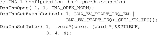
Both methods add cost to our application, since both are using precious resources. Adding one column implies using more RAM, 800 bytes more for the precision. Using a second channel of DMA (out of the four total) seems also a high price to pay. My choice goes to the DMA, though, because to me it seems there’s never enough RAM, and this way we get to experiment with yet another cool feature of the PIC32 DMA controller: DMA channel chaining.
It turns out that there is another friendly function call, DmaChnSetControl(), that can quickly perform just what we need, triggering the execution of a specific channel DMA transfer to the completion of a previous channel DMA transfer. Here is how we link the execution of channel 0 (the one drawing a line of pixels) to the previous execution of channel 1:
![]()
Notice that only contiguous channels can be chained. Channel 0 can be chained only to channel 1; channel 1 can be chained to channel 0 or channel 2 (you decide the “direction” up or down), and so on.
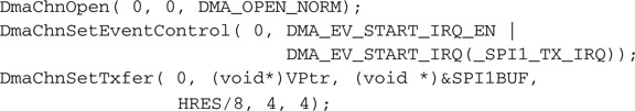
We can now configure the DMA channel 1 to feed the SPI1 module with some more bytes of zero; four more will take our total back-porch time to 7us:
The symbol zero, used here could be a reference to a 32-bit integer variable that needs to be initialized to zero or an array of such integers to allow us to extend the back porch and further center the image on the screen.
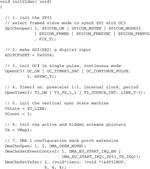
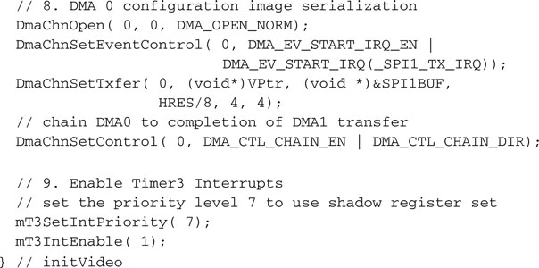
Now that we have identified all the pieces of the puzzle, we can write the complete initialization routine for all the modules required by the video generator:
Completing a Video Library
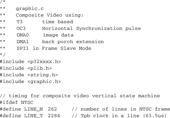
We can now complete the coding of the entire video state machine, adding all the definitions and pin assignments necessary:
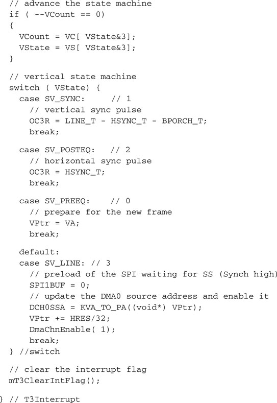
Notice how at the beginning of each line containing actual image data (SV_LINE) we update the DMA source pointer (DCH0SSA) to point to the next line of pixels, but in doing so, we take care to translate the address to a physical address using the KVA_TO_PA() inline function, which involves a simple bit-masking exercise. As you can understand, the DMA controller does not need to be concerned with the way we have remapped the memory and the peripheral space; it demands a physical address. Normally it is the DMA library that takes care of such a low-level detail, and we could have once more used the DmaChnSetTxfer() function to get the job done, but I could not help it—I just needed an excuse to show you how to directly manipulate the DMA controller registers and in the process save a few instruction cycles.
To make it a complete graphic library module, we need to add a couple of accessory functions, such as:
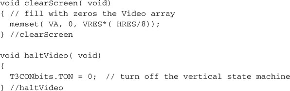
In particular, clearScreen() will be useful to initialize the image memory map, the VMap array. However, haltvideo() will be useful to suspend the video generation, should an important task/application require 100 percent of the PIC32 processing power.
Save all the preceding functions in a file called graphic.c and place it in our lib directory, I can foresee an extensive use of its functions in this and the next few chapters. Also add this file to a new project called Video.
Then create a new file and add the following definitions:
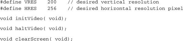
Notice how the horizontal resolution and vertical resolution values are the only two parameters exposed. Within reasonable limits (due to timing constraints and the many considerations exposed in the previous sections), they can be changed to adapt to specific application needs, and the state machine and all other mechanisms of the video generator module will adapt their timing as a consequence.
Save this file as graphic.h and add it to the common include directory.
Testing the Composite Video
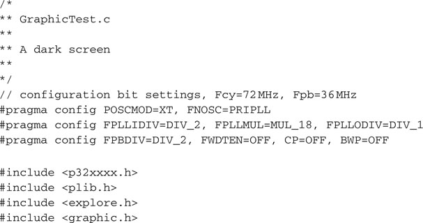
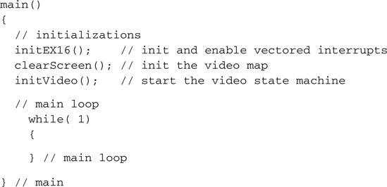
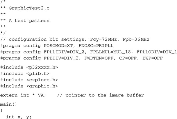
To test the composite video module we have just completed, we need only the MPLAB SIM simulator tool and possibly a few more lines of code for a new main module, to be called GraphicTest.c:
Remember to add the explore.c module from the lib directory, then save the project and use the Build Project checklist to build and link all the modules.
Open the Logic Analyzer window and use the Logic Analyzer checklist to add the OC3 signal (sync) and the SDO1 (video) to the analyzer channels.
At this point you could run the simulator for a few seconds and, after pressing the halt button, switch to the Logic Analyzer output window to observe the results (see Figure 13.15). The trace memory of the simulator is of limited capacity (unless you have configured it to use the extended buffers) and can visualize only a small subset of an entire video frame. In other words, it is very likely that you will be confronted with a relatively uninteresting display containing a regular series of sync pulses. Unfortunately, the MPLAB SIM simulator does not yet simulate the output of the SPI port, so for that, we’ll have to wait until we run the application on real hardware.
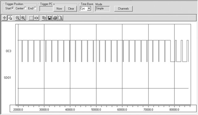
Regarding the sync line, there is one interesting time we would like to observe: that is when we generate the vertical synchronization signal with a sequence of three long horizontal synch pulses at the beginning of each frame. By setting a breakpoint on the first line of the SV_POSTEQ state inside the Timer3 interrupt service routine, you can make sure that the simulation will stop close to the beginning of a new frame.
You can now zoom in the central portion to verify the proper timing of the sync pulses in the pre/post and vertical sync lines (see Figure 13.16).

Keep in mind that the Logic Analyzer window approximates the reading to the nearest screen pixel, so the accuracy of your reading will depend on the magnification (improving as you zoom in) and the resolution of your PC screen. Naturally, if what you need is to determine with absolute precision a time interval, the most direct method is to use the Stopwatch function of the MPLAB SIM software simulator together with the appropriate breakpoint settings.
Measuring Performance
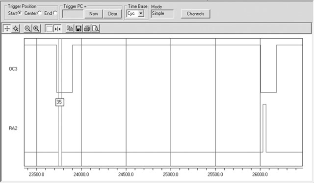
It might be interesting to get an idea of the actual processor overhead caused by the video module. Using the Logic Analyzer we can visualize and attempt to estimate the percentage of time the processor spends inside the interrupt service routine.
As we did before, we will use a pin of PORTA (RA2) as a flag that will be set to indicate when we are inside the interrupt service routine and cleared when we are executing the main loop.
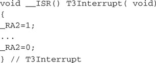
After recompiling and adding RA2 to the channels captured by the Logic Analyzer tool (see Figure 13.17), we can zoom in a single horizontal line period. Using the cursors, we can measure the approximate duration of an interrupt service routine. We obtain a value of 35 cycles out of a line period of 2284 cycles, representing an overhead of less than 1.5 percent of the processor time—a remarkable result due in great part to the support of the DMA controller!
Seeing the Dark Screen
Playing with the simulator and the Logic Analyzer tool can be entertaining for a little while, but I am sure at this point you will feel an itch for the real thing! You’ll want to test the video interface on a real TV screen or any other device capable of receiving an composite video signal, connected with the simple (resistors only) interface to an actual PIC32. If you have an Explorer 16 board, this is the time to take out the soldering iron and connect the three resistors to a standard RCA video jack using the small prototyping area in the top-right corner of the demo board. Alternatively, if you feel your electronic hobbyist skills are up to the task, you could even develop a small PCB for a daughter board (a PICTail™) that would fit in the expansion connectors of the Explorer 16.
Check the companion Web site (www.pic32explorer.com) for the availability of expansion boards that will allow you to follow all the advanced projects presented in the third part of the book.
Whatever your choice, the experience will be breathtaking.
Or … not (see Figure 13.18)! In fact, if you wire all the connections just right, when you power up the Explorer 16 board you are going to be staring at just a blank or, I should say, “black” screen. Sure, this is an achievement; in fact, this already means that a lot of things are working right, since both the horizontal and vertical synchronization signals are being decoded correctly by the TV set and a nice and uniform black background is being displayed.

Test Pattern
To spice things up, let’s start filling that video array with something worth looking at, possibly something simple that can give us immediate feedback on the proper functioning of the video generator. Let’s create a new test program as follows:

Instead of calling the clearScreen() function, this time we used two nested for loops to initialize the VMap array. The external (y) loop counts the vertical lines, and the internal (x) loop moves horizontally, filling the eight words (each containing 32 bits) with the same value: the line count. In other words, on the first line, each 32-bit word will be assigned the value 0; on the second line, each word will be assigned the value 1, and so on until the last line (200th), where each word will be assigned the value 199 (0x000000C7 in hexadecimal).
If you build the new project and test the video output you should be able to see the pattern shown in Figure 13.19.
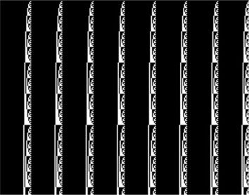
In its simplicity, there is a lot we can learn from observing the test pattern. First, we notice that each word is visually represented on the screen in binary, with the most significant bit presented on the left. This is a consequence of the order used by the SPI module to shift out bits: that is, MSb first. Second, we can verify that the last row contains the expected pattern, 0x000000c7, so we know that all rows of the memory map are being displayed. Finally, we can appreciate the detail of the image. Different output devices (TV sets, projectors, LCD panels, and so on) will be able to lock the image more or less effectively and/or will be able to present a sharper image, depending on the actual display resolution and their input stages bandwidth. In general, you should be able to appreciate how the PIC32 can generate effectively straight vertical lines. This is not a trivial achievement.
This does not mean that on the largest screens you will not be able to notice small imperfections here and there as small echoes and possibly minor visual artifacts in the output image. Realistically, the simple three-resistor interface can only take us so far.
Ultimately the entire composite video signal interface could be blamed for a lower-quality output. As you might know, S-Video, VGA, and most other video interfaces keep luminance and synchronization signals separate to provide a more stable and clean picture.
Plotting
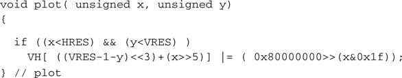
Now that we are reassured about the proper functioning of the graphic display module, we can start focusing on putting it to good use. The first natural step is to develop a function that allows us to light up one pixel at a precise coordinate pair (x, y) on the screen. The first thing to do is derive the line number from the y coordinate. If the x and y coordinates are based on the traditional Cartesian plane representation, with the origin located in the bottom-left corner of the screen, we need to invert the address before accessing the memory map so that the first row in the memory map corresponds to the y maximum coordinate VRES-1 or 199 while the last row in the memory map corresponds to the y coordinate 0. Also, since our memory map is organized in rows of eight words, we need to multiply the resulting line number by 32 to obtain the address of the first word on the given line. This can be obtained with the following expression:
![]()
where VH is a pointer to the image buffer.
Pixels are grouped in 32-bit words, so to resolve the x coordinate we first need to identify the word that will contain the desired pixel. A simple division by 32 will give us the word offset on the line. Adding the offset to the line address as we calculated will provide us with the complete word address inside the memory map:
![]()
To optimize the address calculation, we can use shift operations to perform the multiplication and divisions as follows:
![]()
To identify the bit position inside the word corresponding to the required pixel, we can use the reminder of the division of x by 32, or more efficiently, we can mask out the lower 5 bits of the x coordinate. Since we want to turn the pixel on, we will need to perform a binary OR operation with an appropriate mask that has a single bit set in the corresponding pixel position. Remembering that the display puts the MSb of each word to the left (the SPI module shifts bits MSb first), we can build the mask with the following expression:
![]()
Putting it all together, we obtain the core of the plot function:
![]()
As a final touch we can add “clipping”—that is, a simple safety check, just to make sure that the coordinates we are given are in fact valid and within the current screen map limits.
Add the following few lines of code to the graphic.c module we saved in the lib directory:
By defining the x and y parameters as unsigned integers, we guarantee that, should negative values be passed along, they will be discarded too because they will be considered large integers outside the screen resolution.
Now let’s remember to add the function prototype to the graphic.h file in the includedirectory:
![]()
Watch Out
The plot() function as defined is efficient, but it is not scalable. In other words, if you change the HRES or VRES parameters in the graphic.h file, you will have to rethink the way you compute the address and bit position of a pixel for a given x, y pair of coordinates.
A Starry Night
To test the newly developed plot() function, let’s once more modify the Video project. We will include the graphic.c and graphic.h files, but we will also use the pseudo-random number-generator functions available in the standard C library stdlib.h. By using the pseudo-random number generator to produce random x and ycoordinates for 1,000 points, we will test both the plot() function and, in a way, the random generator itself with the following simple code:
Save the file as GraphicTest3.c and add it to the Video project to replace the previous demo. Once you build the project and program the Explorer 16 board with your in circuit emulator of choice, the output on your video display should look like a nice starry night, as in the screen shot captured in Figure 13.20.
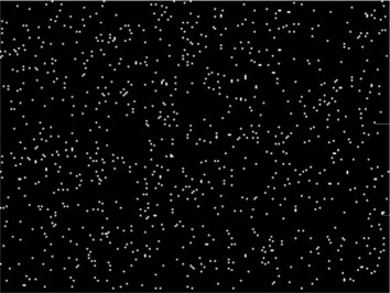
A starry night it is, but not a realistic one, you’ll notice, since there is no recognizable trace of any increased density of stars around a belt—in other words, there is no Milky Way!
This is a good thing! This is a simple proof that our pseudo-random number generator is in fact doing the job it is supposed to do.
Line Drawing
The next obvious step is drawing lines, or I should say line segments. Granted, horizontal and vertical line segments are not a problem; a simple for loop can take care of them. But drawing oblique lines is a completely different thing. We could start with the basic formula for the line between two points that you will remember from school days:
![]()
where (x0,y0)and (x1,y1) are, respectively, the coordinates of two generic points that belong to the line.
This formula gives us, for any given value of x, a corresponding y coordinate. So we might be tempted to use it in a loop for each discreet value of x between the starting and ending point of the line, as in the following example:
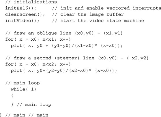
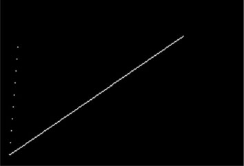
The output produced (Figure 13.21) is an acceptably continuous segment only for the first (shallower) line, where the horizontal distance (x1-x0) is greater than the vertical distance (y1-y0). In the second, much steeper, line, the dots appear disconnected and we are clearly unhappy with the result. Also, we had to perform floating-point arithmetic, a computationally expensive proposition compared to integer arithmetic, as we have seen in previous chapters.
Bresenham Algorithm
Back in 1962, when working at IBM in the San José development lab, Jack E. Bresenham developed a line-drawing algorithm that uses exclusively integer arithmetic and is today considered the foundation of any computer graphic program. Its approach is based on three optimization “tricks”:
The resulting line-drawing code is compact and extremely efficient; here is an adaptation for our video module:
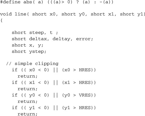
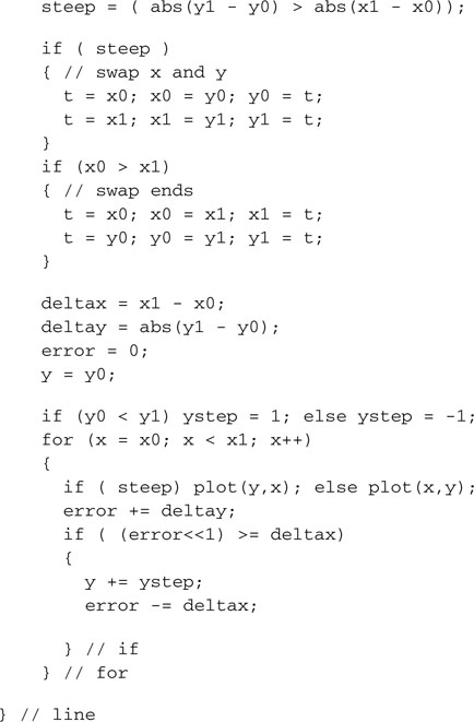
We can add this function to the video module graphic.c and add its prototype to the include file graphic.h:
![]()
To test the efficiency of the Bresenham algorithm, we can create a new small project and, once more, use the pseudo-random number-generator function. The following example code will first draw a frame around the screen and then exercise the line-drawing routine, producing 100 lines at randomly generated coordinates:
The main loop also uses the getKey() function, developed in the previous chapters and added to the explore.h module, to wait until a button is pressed before the screen is cleared and a new set of 100 random lines is drawn on the screen (see Figure 13.22 ).
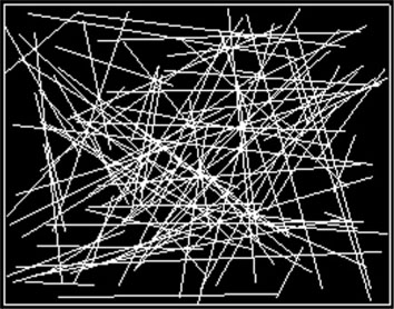
You will be impressed by the speed of the line-drawing algorithm. Even when increasing the number of lines drawn to batches of 1,000, the PIC32 performance will be apparent.
Plotting Math Functions
With the completed graphic module we can now start exploring some interesting applications that can take full advantage of its visualization capabilities. One classical application could be plotting a graph based on data logged from a sensor, or more simply for our demonstration purposes, calculated on the fly from a given math function.
For example, let’s assume that the function is a sinusoid (with a twist), as in the following:
![]()
Let’s also assume that we want to plot its graph for values of x between 0 and 8*PI.
With minor manipulations, we can scale the function to fit our screen, remapping the input range from 0 to 200 and the output range to the +75/-75 value range.
The following program example will plot the function after tracing the x and y axes:
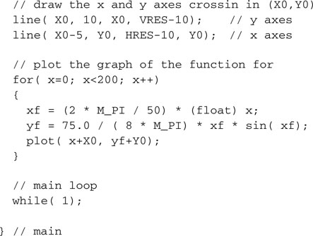
Notice the inclusion of the math.h library to obtain the prototypes of the sin() function and some useful definitions, among which is the value of pi, or I should say M_PI.
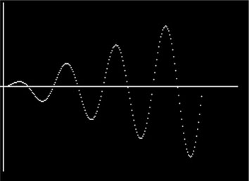
Save the file as graphld.c and replace it as the main module of the Video project. Build the project and program the Explorer 16 board with your in-circuit debugger of choice. Quick, the new function graph will appear on the screen (see Figure 13.23)!
Should the points on the graph become too sparse, we have the option now to use the line-drawing algorithm to connect each point to the previous one.
Two-Dimensional Function Visualization
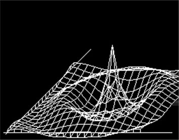
More interesting and perhaps entertaining could be plotting two-dimensional function graphs. This adds the thrill of managing the perspective distortion and the challenge of connecting the calculated points to form a visually pleasant grid.
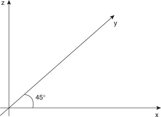
The simplest method to squeeze the third axis in a two-dimensional image is to utilize what is commonly known as an isometric projection, a method that requires minimal computational resources while providing a small visual distortion. The following formulas applied to the x, y, and z coordinates of a point in a three-dimensional space produce the px and py coordinates of the projection on a two-dimensional space (our video screen; see Figure 13.24).
![]()
To plot the three-dimensional graph of a given function: z = f(x,y) we proceed on a grid of points equally spaced in the x and y plane using two nested for loops. For each point we compute the function to obtain the z coordinate, and we apply the isometric projection to obtain a (px,py) coordinate pair. Then we connect the newly calculated point with a segment to the previous point on the same row (previous column). A second segment needs to be drawn to connect the point to a previously computed point in the same column and the previous row (see Figure 13.25).
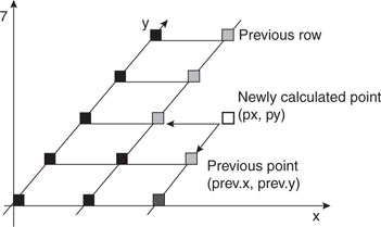
Although it is a trivial task to keep track of the coordinates of the previously computed point on the same row, recording the coordinates of the points on “each” previous row might require significant memory space. If, for example, we are using a grid of 20 × 20 points, we would need to store the coordinates of up to 400 points. Requiring two integers each, that would add up to 800 words, or 3,200 bytes of precious RAM. In reality, as should be evident from the preceding picture, all we really need is the coordinates of the points on the “edge” of the grid as painted so far. Therefore, with a little care, we can reduce the memory requirement to just 20 coordinate pairs by maintaining a small (rolling) buffer.
The following example code visualizes the graph of the function:
![]()
for values of x and y in the range - 3* PI to +3*PI:
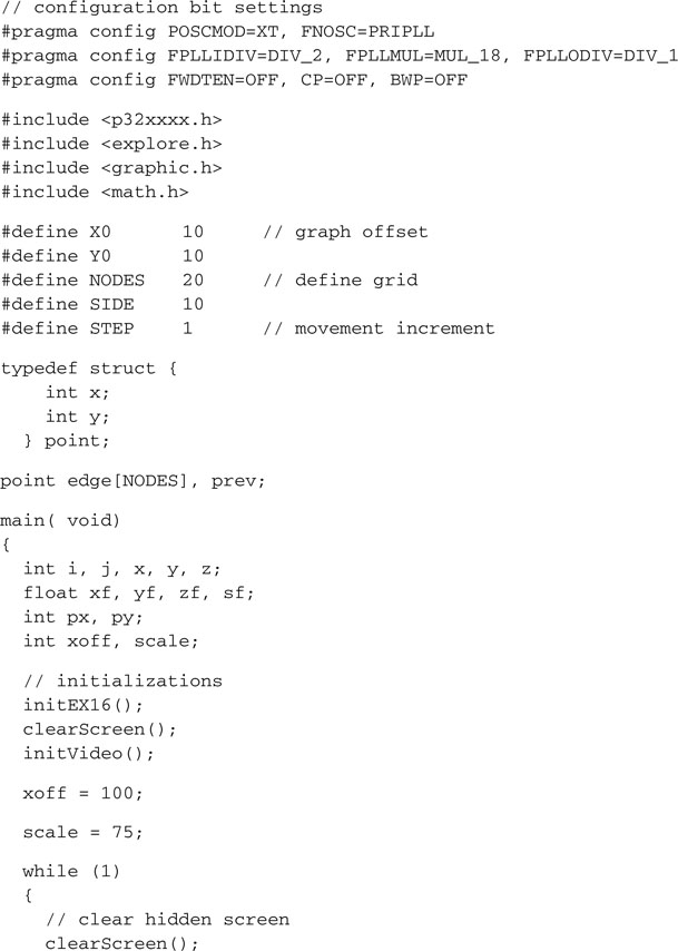
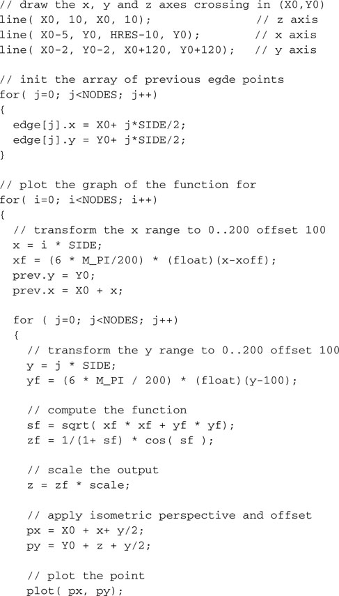
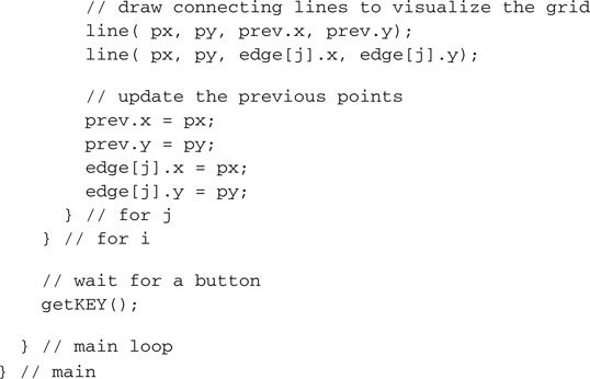
Save the file as graph2d.c and replace it in the Video project as the main source. After building the project and programming the Explorer 16 demo board, you will notice how quickly the PIC32 can produce the output graph, although significant floating-point math is required because the function is applied sequentially to 400 points and as many as 800 line segments are drawn on the video (see Figure 13.26).
Fractals
Fractals is a term coined by Benoit Mandelbrot, a mathematician and fellow researcher at the IBM Pacific Northwest Labs, back in 1975 to denote a large set of mathematical objects that presented an interesting property: that of appearing self-similar at all scales of magnification, as though constructed recursively with an infinite level of detail. There are many examples of fractals in nature, although their self-similarity property is typically extended over a finite scale. Examples include clouds, snowflakes, mountains, river networks, and even the blood vessels in our bodies.
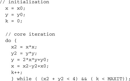
Since it lends itself to impressive computer visualizations, the most popular example of mathematical fractal object is perhaps the Mandelbrot set. It’s defined as a subset of the complex plane where the quadratic function z2 + c is iterated. By exclusion, points c of the complex plane for which the iteration does not “diverge” are considered to be part of the set. Since it is easy to prove that once the modulus of z is greater than 2, the iteration is bound to diverge; hence the given point is not part of the set, we can proceed by elimination. The problem is that as long as the modulus of z remains smaller than 2,we have no way of telling when to stop the iteration and declare the point part of the set. So, typically, computer algorithms that depict the Mandelbrot set use an approximation by setting an arbitrary maximum number of iterations past which a point is simply assumed to be part of the set.
Here is an example of how the inner iteration can be coded in C language:
![]()
where x0 and y0 are the coordinates in the complex space of the point c.
We can repeat this iteration for each point of a squared subset of the complex plane to obtain an image of the entire Mandelbrot set. The considerations we made on the modulus of c imply that the entire set must be contained in the disc of radius 2 centered on the origin, so, as we develop a first program, we will scan the complex plan in a grid of HRES xVRES points (to use the fullscreen resolution of our video module), making sure to include the entire disc:
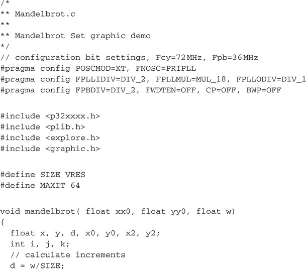
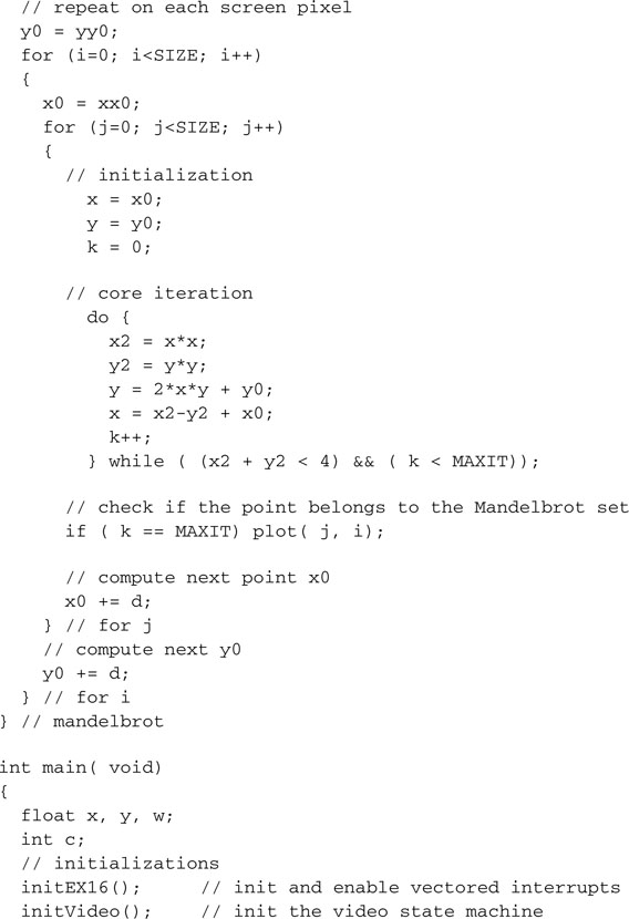
Save this file as Mandelbrot.c and add it to a new project that we will call Mandelbrot. Make sure that all the other required modules are added to the project too, including graphic.c, graphic.h, and explore.c. Build the project, program the Explorer 16 board using your in-circuit debugger of choice, and if all is well, when you let the program run you will see the so-called Mandelbrot “cardiod” appear on your screen (see Figure 13.27).

I will confess that since when, as a kid, I bought my first personal computer—actually, home computer was the term used back then for the Sinclair ZX Spectrum—I have been playing with fractal programs. So I have a vivid memory of the long hours I used to spend staring at the computer screen, waiting for the old trusty ZX80 processor (running at the whopping speed of 3.5 MHz) to paint this same images. A few years later, my first IBM PC, an XT clone running on a 8088 processor at a not much higher clock speed of 4 MHz, was not faring much better and, although the screen resolution of my monochrome Hercules graphic card was higher, I would still launch programs in the evening to watch the results the following morning after what amounted sometimes to up to eight hours of processing.
WOW
Clearly, the amount of computation required to paint a fractal image varies enormously with the chosen area and the number of maximum iterations allowed (MAXIT), but, although I have seen this program run by several other processors, including the PIC24 (at 32 MHz), the first time I saw the PIC32 paint the cardiod in less than 5 seconds, I got really excited again!
The real fun has just begun. The most interesting parts of the Mandelbrot set are at the fringes, where we can increase the magnification and zoom in to discover an infinitely complex world of details. By visualizing not just the points that belong to the set but also the ones that diverge at its edges, and by assigning each point a “color” that depends on how fast they do diverge, we can further improve “aesthetically” the resulting image. Since we have only a monochrome display, we will simply use alternate bands of black and white assigned to each point according to the number of iterations it took before it either reached the maximum modulus or the maximum number of iterations. Simply enough, this means we will have to modify just one line of code from our previous example:
![]()
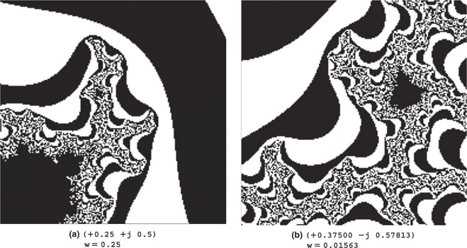
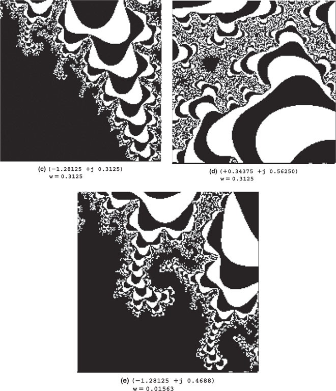
Also, since the best way to play with Mandelbrot sets is to explore them by selecting new areas and zooming in the details, we can modify the main program loop to let us select a portion of the image by pressing one of the four buttons on the Explorer 16 board. We can imagine splitting the image into four corresponding quadrants, numbered clockwise starting from the top left, and doubling the resolution by halving the grid dimension (w) ( see Figure 13.28 ).
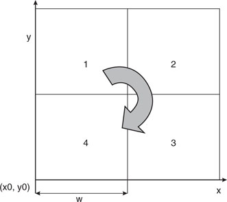
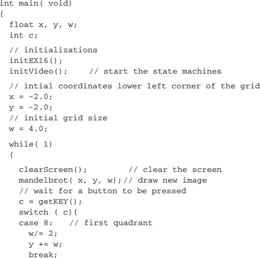
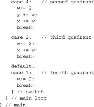
Figure 13.29 shows a selection of interesting areas you will be able to explore with a little patience.
Text
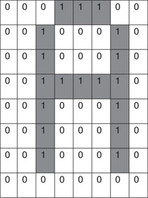
So far we have been focusing on simple graphical visualizations, but on more than one occasion you might feel the desire to actually augment the information presented on the screen with some text. Writing text on the video memory is no different than plotting points or drawing lines; in fact, it can be achieved using a variety of methods, including the plotting and line-drawing functions we have already developed. But for greater performance and to require the smallest possible amount of code, the easiest way to text on our graphic display is to develop a fixed spacing font. Each character can be drawn in an 8 × 8 pixel box; this way 1 byte will encode each row and 8 bytes will encode the entire character. We can then assemble a basic set of alphabetical, numerical, and punctuation characters, using the order in which they are appear in the ASCII character set, as a single array of char integers that will constitute our simple font (see Figure 13.30).
To save space, we don’t need to create the first 32 codes of the ASCII set that correspond mostly to commands and special synchronization codes used by teletypewriters and modems of the old days.
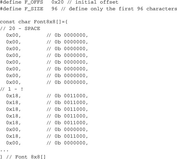
Notice that the Font8x8[] array is defined with the attribute const because its contents are supposed to remain (mostly) unchanged during the execution of the program, and it is best allocated in the Flash memory of the PIC32 to save precious RAM memory space.
Of course, the definition of the shape of each character can be a matter of personal taste. You are welcome to modify the Font8x8[] array contents to suit your preferences.
Note
Defining a new font is a long and detailed work, but it is one that gives a lot of space to creativity, and I know that some of you will find it pretty entertaining. A complete listing of the font.h file would waste several pages of this book, so I decided to omit it here. You can find it on the companion CD-ROM.
Printing a character on the screen is now a matter of copying 8 bytes from the font array to the desired position on the screen. In the simplest case, characters can be aligned to the words that compose the image buffer of the graphics module. In this way the character positions are limited to 32 characters per line (256/8, assuming HRES = 256) and a maximum of 25 rows of text could be displayed (200/8, assuming VRES = 200).
A more advanced solution would call for absolute freedom in positioning each character at any given pixel coordinate. This would require a type of manipulation, often referred to as BitBLT (an acronym that stands for bit block transfer) that is common in computer graphics, particularly in video game design. In the following we will stick to the simpler approach. looking for the solution that requires the smallest amount of resources to get the job done.
Printing Text on Video
When printing text on video we need the assistance of a cursor, a virtual placeholder to keep track of where on the screen we are going to place the next character. As we print, it is easy to advance the cursor to mimic somewhat the behavior of a typewriter as it zigzags across the sheet and as it scrolls the paper.
OOPS
As I am writing this, it occurs to me that many of you might have never used a typewriter in real life and that the beauty of this parallel is going to be totally lost on you. Maybe it feels like I might be talking of reed pens and kalamoi or parchment …
Our cursor will be made of two integers, holding the x and y of a new coordinate system that is now upside down with respect to the traditional Cartesian orientation and much more coarse as it counts rows and columns rather than individual pixels:
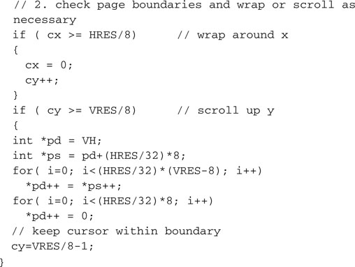
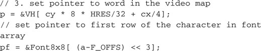
To print one ASCII character on the screen at the current cursor position, we will create the putcv() function that will perform the following simple steps:
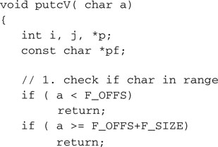
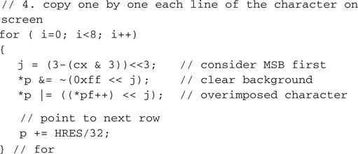
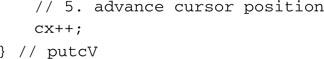
Add this function to the bottom of the graphic.c module and its prototype to the bottom of the graphic.h include file:
![]()
For our convenience we can now create a small function that will print an entire (zero-terminated) ASCII string on the screen:
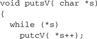
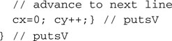
Add this function to the graphic.c library module and its prototype to the graphic.h:
![]()
Since we’re at it, let’s add a couple more useful macros to the graphic.h file:
Text Test
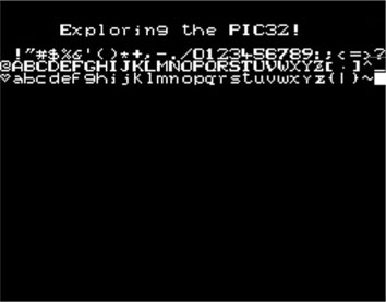
To quickly test the effectiveness of the new text functions, we can now create a short program that, after printing a small banner on the first line of the screen, will print out each character defined in the 8 ×8 font:
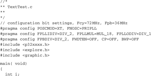
Save this file as TextTest.c and add it to a new project that we will call TextTest. Make sure that all the other required modules are added to the project too, including graphic. c, graphic.h, and explore.c. Build the project, program the Explorer 16 board using your in-circuit debugger of choice, and if all is well, when you run you will see the screen come alive with a nice welcome message (see Figure 13.31).
The Matrix Reloaded
To further test the new text page video module, we will modify an example we saw in a previous chapter: the Matrix. Back then, we were using the asynchronous serial communication module (UART1) to communicate with a VT100 computer terminal or, more likely, a PC running the HyperTerminal program configured for emulation of the historical DEC VT100 terminal’s protocol. Now we can replace the putcU() function calls used to send a character to the serial port, with putcV() function calls directed to the graphic interface.
Let’s modify the TextTest project by replacing the TextTest.c main module with the new Matrix2.c module, modified as follows:
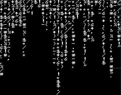
After saving and building the project, program the Explorer 16 board using your incircuit debugger of choice and run the program (see Figure 13.32). You will notice how much faster the screen updates can be compared because the program now has direct access to the video memory and no serial connection limits the information transfers (as fast as the 115,200 baud connection was in our previous demo project; that was our bottleneck). The demo will run so fast that you will need to add a delay of a few extra milliseconds to give your eyes time to focus.
![]()
Debriefing
Today we have explored the possibility of producing a video output using a minimal hardware interface composed in practice of only three resistors. We learned to use four peripheral modules together to build the complex mechanism required to produce a properly formatted NTSC composite video signal. Combining a 16-bit-timer, an output compare module, one SPI port, and a couple of channel of the DMA module we have obtained video capabilities at the cost of just 1.5% processor overhead. After developing basic graphic functions to plot individual pixels first and efficiently draw lines, we explored some of the possibilities offered by the availability of a graphic video output, including unidimensional and two-dimensional function graphing. We completed our explanations with a brief foray in the world of fractals and learning to display text on top of graphics.
Notes for the PIC24 Experts
The OC module of the PIC32 is mostly identical to the PIC24 peripheral, yet some important enhancements have been included in its design. Here are the major differences that will affect your code while porting an application to the PIC32:
Tips & Tricks
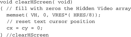
The final touch, to complete our brief excursion into the world of graphics, would be to add some animation capabilities to our graphic libraries. To make the motion fluid and avoid an annoying flicker of the image on the screen, a technique known as double buffering is often used. This requires the allocation of two image buffers of identical size. One, the “active” buffer, is shown on the screen; the other, the “hidden” buffer, is where the drawing takes place. When the drawing on the hidden buffer is completed, the two are swapped. What used to be the active buffer is not visible anymore. The (now) hidden buffer can be cleared without fear of producing any flicker, and the drawing process can restart.
With the current image resolution settings (256 × 200), the RAM usage grows to a total of 12,800 bytes (256*200*2/8), which represents only approximately 40 percent of the total RAM available on the PIC32MX360.
To extend our graphic libraries and support double buffering, we can implement the following simple modifications:
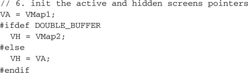
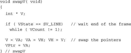
Notice that care must be taken not to perform the swap in the middle of a frame but synchronized with the end of one frame and the beginning of the next.
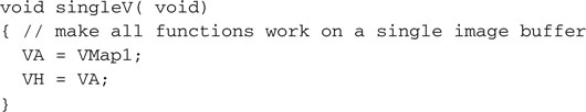
One last utility function can be added for all those cases when the animation needs to be suspended and the display has to return to a simple buffering mode:
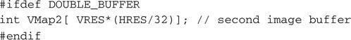
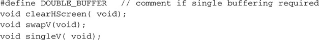
Remember to add all the corresponding function prototypes to the graphic.h include file and additionally, at the top, declare the new symbol DOUBLE_BUFFER:
Note
All the examples developed in this chapter and the previous one can now be recompiled using the newly extended graphic modules with the condition that the DOUBLE_BUFFER declaration is either commented out or the singleV() function is called immediately after the initVideo() call!
Exercises
Books
Mandelbrot, Benoit, B., The Fractal Geometry of Nature(W. H. Freeman, 1982). This is “the” book on fractals, written by the man who contributed most to the rediscovery of fractal theory.
Hofstadter, Douglas, Godel, Escher, Bach: An Eternal Golden Braid, 20th Anniversary Edition (Basic Books, 1999). One of the most inspiring books in my library. At 777 pages, it’s not easy reading, but it will take you on a journey through graphics, math, and music and the surprising connections among the three.
Links
http://en.wikipedia.org/wiki/Fractals. A starting point for you to begin the online exploration of the world of fractals.
http://en.wikipedia.org/wiki/Zx_spectrum. The Sinclair ZX Spectrum was one of the first personal computers (home computers, as they used to be called) launched in the early 1980s. Its graphic capabilities were very similar to those of the graphic libraries we developed in this project. Although it used several custom logic devices to produce a video output, its processing power was less than a tenth that of the PIC32. Still, the limited ability to produce color (only 16 colors with a resolution of a block of 8 × 8 pixels) enticed many programmers to create thousands of challenging and creative video games.