INVESTMENT BENCHMARKS

My favorite definition of a growth stock is
“a stock that somebody is trying to sell you.”

—BURTON CRANE

A stock’s intrinsic value equals the present value of its dividends, but value investors look beyond dividends to a firm’s earnings and assets. Earnings are important because these give firms the means to pay dividends, and assets are important because these are the source of earnings. Dividend-price ratios, earnings-price ratios, and asset-price ratios are sensible financial benchmarks, but none are infallible.

THE EARNINGS-PRICE RATIO

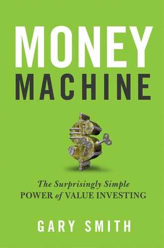
A stock’s earnings-price ratio (E/P), or earnings yield, is a rough estimate of a stock’s rate of return. If a stock sells for $100 a share and the company earns $10 a share, it seems as though the shareholders have earned $10, which is a 10 percent return on their investment. If so, earnings yields should be related closely to the interest rates on Treasury bonds.

Figure 7-1 shows the S&P 500 earnings yield and the interest rate on long-term Treasury bonds back to 1871. There does not appear to be a consistent relationship. One thing that does stand out is how volatile earnings yields have been compared to interest rates, a reflection of the collective euphoria and hysteria that periodically seizes the stock market. Mr. Market is fickle.

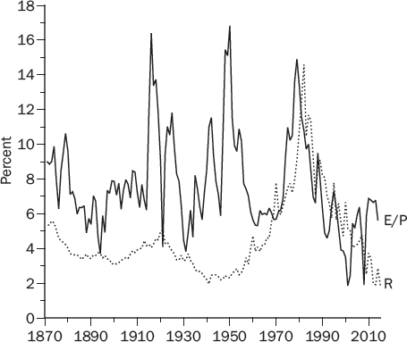
The earnings yield was well above the Treasury rate up until the 1960s. Figure 7-2 zooms in on the years since 1960. Over the last fifty years, these two series have been more closely aligned, but they hardly move in unison. Sometimes they even move in opposite directions. After 2010, the Treasury rate dropped while the earnings yield rose, creating a substantial gap between the two.

The problem with interpreting the earnings yield as the shareholders’ return is that stockholders receive dividends, not earnings. Getting a $10 dividend is a lot different from reading about $10 in earnings in the annual report.

If a company pays a $5 dividend out of its $10 earnings, stockholders should consider the fate of the remaining $5. If these retained earnings are squandered, the $5 might as well not have been earned in the first place. For a dollar of retained earnings to be worth a dollar to shareholders, the firm must earn a return equal to the shareholders’ required return. If the firm earns less than the required return, a dollar of retained earnings is worth less than a dollar. If the firm earns more than the required return, a dollar of retained earnings is worth more than a dollar. This is why Berkshire Hathaway doesn’t pay dividends. Its managers believe that their investments will earn more than their shareholders’ required return.

The more general point is that the earnings-price ratio is an imperfect measure of the stockholders’ return. Earnings are important because they are the source of dividends. However, earnings are the means to the end, not the end itself.

THE DIVIDEND-PRICE RATIO

Some investors use the dividend yield, the ratio of dividends per share to price (D/P), as a measure of the shareholders’ return. In our example, investors see the stock’s $5 dividend and $100 price, and they estimate the stock’s return to be 5 percent. However, this calculation only makes sense if the dividend stays at $5 indefinitely. A $5 dividend, year after year, on a $100 investment is, indeed, a 5 percent return. However, most firms grow with the economy and their earnings and dividends grow, too.

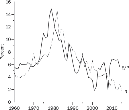
Figure 7-3 shows the history of the S&P 500 dividend yield and the interest rate on long-term Treasury bonds. As with the earnings yield, there is no consistent relationship. It is very interesting, though, that the dividend yield was always above the bond rate before 1958 and persistently below afterward, until they converged in 2009.

In 1950, for example, stocks had a dividend yield of nearly 9 percent when long-term Treasury rates were only 2 percent. Investors either woefully underestimated the likelihood that dividends would grow over time, providing a double-digit return from stocks, or they were so afraid of stocks that they required double-digit returns to persuade them to leave the safety of 2 percent Treasuries. The former explanation is more plausible. What a great time to be a value investor!

A BETTER ALTERNATIVE

The earnings yield looks at profits rather than dividends. The dividend yield ignores the future growth of dividends. A better rule of thumb is to use the insight provided by the JBW equation that was introduced in Chapter 6: The total return equals the dividend yield plus the growth rate of dividends:

We can apply this equation to the overall market by calculating the current dividend yield for the S&P 500 and making an assumption about the long-run growth of dividends, which is perhaps equal to the long-run growth of the economy. This total return estimate—the dividend yield plus the dividend growth rate—can be compared to the interest rate on long-term Treasury bonds plus whatever risk premium seems appropriate. In 1950, for example, a 9 percent dividend yield plus a 5 percent growth rate implies a 14 percent total return, R = 0.09 + 0.05 = 0.14, far above the 2 percent interest rate on long-term Treasury bonds. Value investors were, no doubt, ecstatic about an anticipated 14 percent annual return.

The comparison was much closer in 2013, when the dividend yield and long-term Treasury rate were both around 2 percent. Now, a 5 percent projected growth rate gives stocks a 5 percent margin over Treasuries (7 percent versus 2 percent), which might not be enough for value investors requiring more than a 5 percent risk premium. I was satisfied with a 5 percent premium and wrote a blog saying so.

THE PRICE-EARNINGS RATIO

A stock’s price-earnings ratio is obtained by dividing the price per share by the annual earnings per share. The price-earnings ratio, P/E, is the inverse of the earnings yield, E/P, and its mechanical usage to gauge whether stocks are cheap or expensive is subject to the same cautions.

Many investors have long considered a P/E ratio of 10 as normal and the purchase of a stock with a P/E ratio less than 10 a sound investment. For example, Burton Crane, a New York Times financial writer from 1937 to 1963, observed that “most of us over the age of forty, unless we are completely without market knowledge, subconsciously think of [dividend] yields of 6 per cent and price-earnings ratios of 10 as about right.”

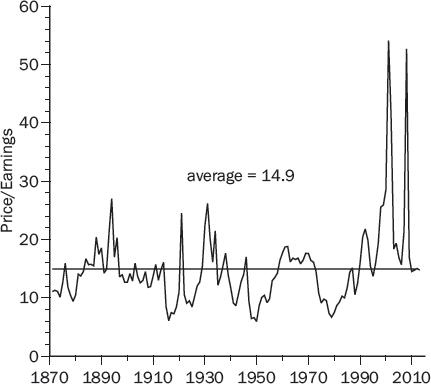
Figure 7-4 shows that the price-earnings ratio for the S&P 500 has varied considerably, falling to a low of close to 5 in some years and topping 20 in others. The average value has been a P/E ratio of 14.9. The P/E spikes in 2001 and 2008 were due to economic recessions that caused earnings to fall by more than 50 percent. Stock prices fell, too, but not as far as earnings because investors believed that the recession would not last long. With earnings down a lot and prices down a little, the P/E went up.

A LOW P/E IS NOT NECESSARILY A BARGAIN

Crane correctly cautioned that “no market is cheap because the price-earnings ratio is low and no market is dear because the ratio is high.” Mechanical rules ignore perfectly logical reasons why individual stocks or the market as a whole may be cheap even if the P/E ratio is high and expensive even though the P/E is low.

The intrinsic value of a stock is higher if earnings (and dividends) are expected to grow faster. Intrinsic values are also higher if interest rates are low. Thus, the market P/E tends to be high when investors are bullish on the economy and/or interest rates are low.

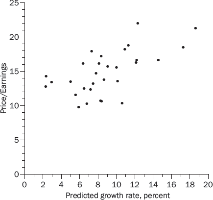
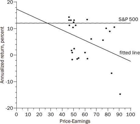
The same is true of individual stocks. Figure 7-5 shows P/E ratios and five-year earnings growth predicted by professional security analysts for the Dow Jones Industrial stocks. Investors were willing to pay more for faster-growing companies.

There are two other factors to consider: short-run fluctuations in earnings and creative accounting. If earnings are depressed temporarily by an economic recession or corporate misfortune, a stock’s price may stay relatively firm as current earnings sag, driving the P/E ratio skyward. In these circumstances, the P/E ratio is unusually high because earnings are abnormally low. In the reverse situation, the P/E will fall if investors perceive a temporary bulge in earnings to be due to extraordinary good luck. Similarly, if investors believe that the firm has used dubious accounting procedures to boost reported earnings, the P/E ratio will be deceptively small because earnings are fictitiously large.

The bottom line is that there is no reason to think that the market’s P/E should be some magic number like 10 or 14.9. There is even less reason to think this should be true of individual stocks.

USING P/ES FOR INVESTMENT DECISIONS

Although it is unwise to base investment decisions on P/E rules carved in stone—for example, buy when the P/E is below 7, sell when it is above 15—price-earnings ratios can still be used to help value investors make informed investment decisions. We will look at a model developed by John C. Bogle, the founder and former chairman of Vanguard. Although his procedure can be used for individual securities and for short horizons, Bogle cautions that there are “two lessons that I have learned in more than a few decades in the investment field. First, the performance of individual securities is unpredictable, period. Second, the performance of portfolios of securities is unpredictable on any short-term basis.”

Thus he recommends using his approach for portfolios (such as the S&P 500) over ten-year horizons. Bogle assumes that intrinsic value is equal to the present value of the cash generated, and that dividends and earnings grow at the same rate. For an investor with a ten-year horizon, this cash consists of the dividends over the next ten years and stock prices ten years from now.

Bogle’s clever insight is that stock prices ten years from now depend on two factors: the growth in earnings and the change in the P/E ratio that the market uses to value these earnings. If earnings double, the stock price will double. If the P/E ratio doubles, the stock price will double. If earnings and the P/E both double, the stock price will quadruple.

This insight also helps us understand why growth stocks are doubly vulnerable. A stock’s price is, by definition, its earnings per share multiplied by its price-earnings ratio. If earnings turn out to be lower than expected, this will reduce the stock price. If the P/E falls because of the disappointing earnings, this will reduce the stock’s price. That’s a double blow to the growth stock’s price.

To implement Bogle’s model, we need to predict the growth rate of earnings and the change, if any, in the price-earnings ratio. We can then estimate the implied rate of return using this simple approximation:

Bogle gives this example for the S&P 500 in the 1980s. At the start of the decade, the dividend yield was 5.2 percent and the P/E was 7.3. Earnings grew at a 4.4 percent rate during this decade and the P/E at the end of the decade was 15.5, an annual growth rate of 7.8 percent. Thus the annual rate of return on the S&P 500 during the 1980s was approximately 17.4 percent:

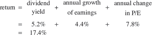
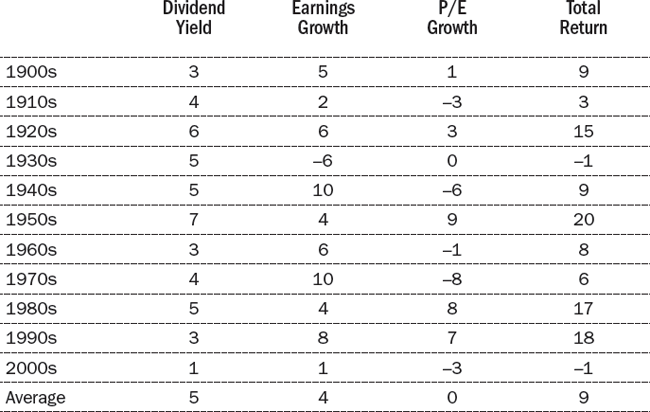
Table 7-1 shows the components of the annual returns for each decade from 1900 through 2010. Stocks did great in the 1950s, 1980s, and 1990s because of extraordinary increases in the P/E ratio. The below-average stock returns in the 1960s, 1970s, and 2000s, in contrast, reflected a falling price-earnings ratio. Overall, the average change in the P/E has been essentially zero. In the long run, half of the return from stocks has been from dividends and half from earnings growth—nothing from changes in the P/E.

SEEING THE DOT-COM BUBBLE

In March 2000, the S&P 500 was four times higher than a decade earlier, a 16 percent annual rate of increase. Add in dividends and investors had made close to 20 percent a year. Easy money! A survey asked investors what annual rate of return they expected over the next ten years. The median answer was 15 percent.

One reason I was convinced that the dot-com boom was a dotcom bubble was an application of Bogle’s model. In the spring of 2000, the S&P 500 had a dividend yield of 1.3 percent and a P/E of 30. Interest rates were 6.4 percent on ten-year Treasury bonds.

Because the future is uncertain, it is a good idea to consider a variety of scenarios. In my investments class, I used Bogle’s model to estimate stock returns over the next ten years for the four scenarios in Table 7-2.

The historical baseline assumed that dividends and earnings would grow by 5 percent a year, as they had over the previous decade, and that the price-earnings ratio would return to its historical average of 15. If so, the shareholders’ annual return would be negative (–1 percent). More pessimistic scenarios implied worse.

The unemployment rate had fallen from 5.6 percent in 1990 to 4.0 percent in March 2000, and it seemed unlikely that the economy would grow faster than it had during the previous decade. An optimistic scenario of 6 percent growth and the P/E rising to 35 would give a 9 percent shareholder return, not much more than the 6.4 percent interest rate on Treasury bonds and a whole lot less than the 15 percent that investors anticipated.

To get that 15 percent return, investors needed to make seemingly delirious assumptions, such as the earnings growth rate rising to 7 percent and the P/E doubling to 60. What would happen when this preposterous future did not materialize and investors learned that stocks were not easy riches? I told my students to expect investors to head for the exits, and most to get trampled.

SEEING THROUGH THE DOOM-AND-GLOOM

The stock market did crash and euphoria turned into hysteria. In December 2008, I was interviewed on a local television show. The S&P 500 was down 40 percent from March 2000 and dot-com stocks were down more—much more. The unemployment rate was 7.8 percent and rising as the economy hurtled into the Great Recession. Who would be crazy enough to buy stocks? I raised my hand.

Here are some excerpts from my interview:

We’re in an economy that’s sick. Everyone is depressed. Everyone is gloomy. Everyone is worried about the future. And yet you gotta think about the prices, how far stock prices have fallen. So, today, you have dividend yields that are close to 4 percent, Treasury bonds are paying 3 percent. Remember back in 2000, Treasury bonds were paying 5 percent more than dividend yields. Now it’s the other way around. Dividend yields are above Treasury bonds. You have price-earnings ratios that are down to 13 or 14.

It reminds me a lot of the 1973–74 crash, which you and I both lived through, and it was just a fearful, fearful time, but 1974 in retrospect was a great time to buy stocks. And then you had the 2000 internet bubble and the crash, 2001–2002, and people were getting out of the market and said they would never go back. In retrospect, 2002 was a great time to buy stocks. . . .

I would say that the worst possible thing to do now if you are in the market is to say I’ve gotta sell everything, I can’t afford to lose any more money. What you’re doing is you’re just locking in your losses.

You and I—we don’t know what stock prices are going to be tomorrow, or next week, or next month, but . . . we can say with great confidence . . . this economy will be much bigger, much stronger ten years from now than it is today, and stock prices will be much higher. And, so, this is a time to be buying, not a time to be panicking. . . .

I’m really excited. I was so gloomy in 2000 and I was so pumped up in 1974 and I was so pumped up in 2002, and I’m pumped up again. I feel like this is a buying opportunity that only comes around a half dozen times in a lifetime.

We’re not yet ten years into December 2008’s future, but the market did recover nicely, with the S&P 500 doubling over the next five years.

SHILLER’S CYCLICALLY ADJUSTED EARNINGS

Nobel laureate Robert Shiller has a sensible way of dealing with short-term fluctuations in earnings. First, he calculates real, inflation-adjusted earnings for the S&P 500. Then he calculates the average value of these inflation-adjusted earnings over the preceding ten years. Figure 7-6 shows that this ten-year average—which he calls cyclically adjusted earnings—smooths out earnings fluctuations caused by temporary booms and recessions.

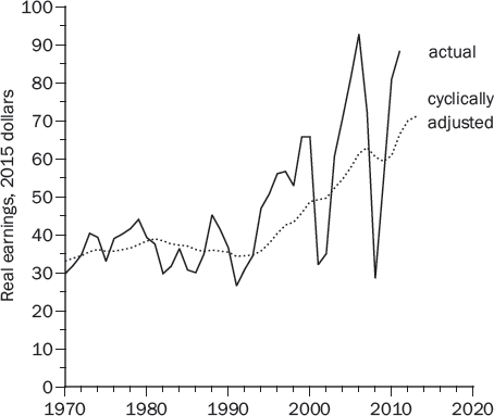
Shiller calculates a cyclically adjusted P/E ratio (CAPE) by dividing the inflation-adjusted value of the S&P 500 by cyclically adjusted earnings. Figure 7-7 shows the actual and cyclically adjusted P/Es for the S&P 500.

This reasonable procedure has the virtue of averaging out booms and busts. However, the cyclically adjusted P/E still has some of the same issues as unadjusted P/Es in gauging whether stocks are cheap or expensive. One is that growth matters. The cyclically adjusted P/E may be unusually high, but still perfectly reasonable, if earnings over the next ten years are expected to be much higher than earnings over the previous ten years.

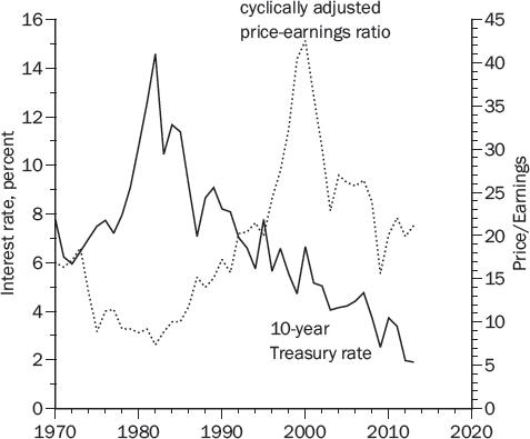
Also, interest rates matter. When interest rates are low, P/E should be high, too. Shiller uses a graph, like the one in Figure 7-8, to demonstrate the inverse relationship between the cyclically adjusted P/E and the interest rate on ten-year Treasury bonds. As interest rates came down from their double-digit levels in the early 1980s, the price-earnings ratio went up.

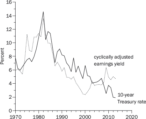
Although the price-earnings ratio P/E is more familiar than the earnings yield E/P, the positive relationship between interest rates and the earnings yield is easier to see than is the negative relationship between interest rates and the price-earnings ratio. Figure 7-9 shows that the cyclically adjusted earnings yield (CAEP) and ten-year Treasury rate have tended to move up and down together.

DID THE STOCK MARKET MAKE A MISTAKE?

The interest rates in Figures 7-8 and 7-9 are not adjusted for inflation. Suppose a one percent increase in the rate of inflation were to increase interest rates and stock dividends, earnings, and prices by one percent. Dollar interest rates would be one percent higher, but inflation-adjusted interest rates and the earnings-price ratio would be constant. These assumptions are surely too simple. Nonetheless, it is reasonable that the earnings yield is more closely related to inflation-adjusted interest rates than to dollar interest rates.

In the spring of 1979, Franco Modigliani and Richard Cohn made the provocative argument that investors in the 1970s mistakenly believed earnings yields should go up and down with dollar interest rates rather than inflation-adjusted interest rates.

A telling example is Benjamin Graham, who recommended a maximum P/E ratio of 15 in the early 1960s, when interest rates on long-term, high-grade corporate bonds were around 4.5 percent, but halved his maximum P/E to 8 in 1974, with corporate bond rates above 9 percent.

Modigliani and Cohn argued that because of this market-wide mistake, stock prices were about half what they should have been, which made earnings yields twice what they should have been.

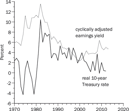
To investigate this argument, I calculated the real inflation-adjusted interest rate each year by using the change in the consumer price index over the next year. For example, I adjusted the dollar interest rate in January 2000 by using the change in the consumer price index between January 2000 and January 2001. This is an imperfect measure of investors’ inflation expectations, but maybe it is not systematically biased.

Figure 7-10 compares these real interest rates with Shiller’s cyclically adjusted earnings yield. What immediately leaps out of this figure is how close they were between 1981 and 2009, and how far apart they were in the 1970s. A comparison of Figures 7-9 and 7-10 confirms the Modigliani-Cohn argument. In the 1970s, investors evidently compared earnings yields with dollar interest rates rather than real interest rates. If this was a mistake, stock prices were much too low in the 1970s.

Although Modigliani and Cohn cautioned that mispriced stocks need not be correctly priced anytime soon, 1979 would have been a very good time to buy stock, as the return from doing so would have been 32 percent in 1980 and 18 percent compounded annually for the entire 1980s.

Part of the reason for the booming market was the drop in interest rates in the 1980s, but part of the reason was that investors made a colossal mistake in the 1970s. This is one of those occasions, like speculative bubbles and panics, where the presumption that markets know best is battered and bruised. It wasn’t a slight mispricing. It was a blunder that left truckloads of $100 bills on the sidewalk.

THE GROWTH TRAP

Decades ago, many investors gauged a stock’s attractiveness by its dividend yield. Indeed, as Figure 7-3 shows, up until 1958 the average dividend yield almost always exceeded the interest rate on Treasury bonds, indicating that investors attached little importance to dividend growth. As late as 1950, the average dividend yield was nearly 9 percent while the yield on Treasury bonds was only 2 percent. The JBW equation teaches us that growth, too, is important. If a stock has a 9 percent dividend yield and the dividend will grow by 5 percent a year, the annual rate of return is 14 percent, not 9 percent.

As the value of growth was increasingly recognized in the 1950s and 1960s, rising stock prices pushed dividend yields below bond yields. By the early 1970s, investors seemed to be interested only in growth, especially the premier growth stocks labeled the Nifty 50. This myopia led them to pay what, in retrospect, were ridiculous prices for growth stocks.

THE NIFTY 50

In the early 1970s, the attention of institutional investors was focused on a small group of “one decision” stocks that were so appealing that they should always be bought and never sold, no matter what the price. Value investors know that it is always a bad idea to buy or sell stocks without considering the price, and this time was no exception.

Among these select few were IBM, Xerox, Disney, McDonald’s, Avon, Polaroid, and Schlumberger. In each case, earnings had grown by at least 10 percent a year over the past five to ten years, and no reason for a slowdown was in sight. Each company was a leader in its field, with a strong balance sheet and profit rates close to 20 percent.

David Dreman recounted the dreams of missed opportunities that danced in investors’ heads:

Had someone put $10,000 in Haloid Xerox in 1960, the year the first plain copier, the 914, was introduced, the investment would have been worth $16.5 million a decade later. McDonald’s earnings increased several thousand times in the 1961–66 period, and then, more demurely, quadrupled again by 1971, the year of its eight billionth hamburger. Anyone astute enough to buy McDonald’s stock in 1965, when it went public, would have made fortyfold his money in the next seven years. An investor who plunked $2,750 into Thomas J. Watson’s Computing and Tabulating Company in 1914 would have had over $20 million in IBM stock by the beginning of the 1970s.

The unfortunate consequence of this fixation on the Nifty 50 was the belief that there is never a bad time to buy a growth stock, nor is there too high a price to pay. A money manager infatuated with growth stocks wrote, “The time to buy a growth stock is now. The whole purpose in such an investment is to participate in future larger earnings, so ipso facto any delay in making the commitment is defeating.” This is suspiciously similar to the Greater Fool Theory and contradicts the main tenet of value investing—that stocks, like groceries, should never be bought without regard for price. IBM is a fine company, but is its stock worth $1,000 a share? Any price, no matter how high?

The subsequent performance of many of the Nifty 50 was disappointing; yet, even today, some money managers believe that you can’t go wrong with a good growth stock, no matter what price you pay. Michael Lipper, president of Lipper Analytical Services, was very blunt: “[Suppose] an investor’s timing was exquisitely wrong and he bought a growth stock at its peak. If he held that stock until the top of the next market cycle, such an investor would be better off with a growth stock than a value play.”

Not necessarily. Avon was a hot growth stock in 1973 when it sold for $140 a share, sixty times earnings. In 1974, the price collapsed to $19; twelve years later, in 1986, it was selling for $25 a share. Polaroid sold for $150 in 1972 (an astounding 115 times earnings), $14 in 1974, and $42 in 1986, before going bankrupt in 2001. Xerox hit $172 in 1972 (sixty times earnings), $49 in 1974, $27 in 1982, and $49 in 1986. An investor with exquisitely wrong timing would have been better off putting money under the mattress, not to mention buying reasonably priced stocks.

These were not isolated cases. Many glamour stocks that were pushed to extraordinary P/E ratios in the 1970s did substantially worse than the market over the next several decades.

There is some uncertainty about the exact composition of the Nifty 50, with one Forbes article referring to a Morgan Guaranty Trust list and several other Forbes articles referring to a Kidder Peabody list. If any group of stocks can be clearly counted among the stocks of the Nifty 50 legend, it is the twenty-four stocks that appear on both lists.

A student and I looked at the performance of these Terrific 24 stocks over the twenty-nine-year period from December 1972 through December 2001. Figure 7-11 shows that eighteen of them underperformed the S&P 500 and that those stocks with the highest P/Es were most likely to underperform. These stocks should be renamed the Terrible 24.

An investor who bought these twenty-four stocks at the end of 1972 would have had 50 percent less wealth at the end of 2001 than an investor who bought the S&P 500.

There are two reasons why growth stocks are sometimes disappointing. First, investors appraising a stock with their hearts instead of their minds see temporary growth and think they have found permanent growth. Second, some growth is worthless and some firms create an appearance of growth to boost the price of their stock. We will look at each of these pitfalls in turn.

THE DANGERS OF INCAUTIOUS EXTRAPOLATION

Benjamin Graham was wary of growth stocks because growth projections are so often based on little more than simple-minded extrapolations: “It must be remembered that the automatic or normal economic forces militate against the indefinite continuance of a given trend. Competition, regulation, the law of diminishing returns, etc. are powerful foes to unlimited expansion.”

The value of a growth stock lies in the distant future, and it is risky to extrapolate a few years of impressive growth into several decades of stunning growth. Many ludicrous examples have been concocted to dramatize the folly of incautious extrapolation. A study of British public speakers over the past 350 years found that the average sentence length had fallen from seventy-two words per sentence for Francis Bacon to twenty-four for Winston Churchill. If this trend continues (famous last words), the number of words per sentence will soon hit zero and then go negative.

It is also an incautious extrapolation to assume that a firm’s extraordinary profits will continue indefinitely.

WORTHLESS GROWTH

Growth per se is not valuable. A company that reduces current dividends in order to grow bigger always increases the firm’s earning growth (as long as profits are positive) but doesn’t increase the intrinsic value of its stock unless the profit is larger than the shareholders’ required return.

Here is a great example of how growth is not necessarily valuable. Consider a mutual fund that invests in Treasury bills—all Treasury bills all the time—paying 4 percent interest. If the fund pays all the interest to its shareholders, they earn a 4 percent return and the fund has a zero percent growth rate. Now suppose the fund switches to a growth philosophy by paying out half the interest to its shareholders and using the other half to buy more Treasury bills. The fund is growing now, but shareholders are no better off—because all the firm did is buy Treasury bills that investors could have purchased themselves.

CREATING AN ILLUSION OF GROWTH

Another trap for investors who focus myopically on earnings growth is that companies can manufacture growth by acquiring companies with low P/E ratios. For a simple example, consider the two firms in Table 7-3, each with $100 million in assets and one million shares outstanding. Smith earns a 10 percent profit on its assets and shareholders require a 10 percent return on their stock. Hwang earns a 20 percent return on its assets and shareholders require a 20 percent return. Both companies pay all of their earnings out as dividends. Both are no-growth companies and each has a total market value of $100 million, $100 a share.

Now assume that Smith merges with Hwang by issuing a million new shares of stock that are traded one-for-one to the Hwang shareholders. The two companies continue to operate exactly as before, the only difference being that their balance sheets are combined. The results are in the last column in Table 7-3. Since there are no changes in their operations or in current and future earnings, the market value of the combined companies should be the sum of the market values of the two separate firms, $100 million + $100 million = $200 million, and the per-share price should stay at $100.

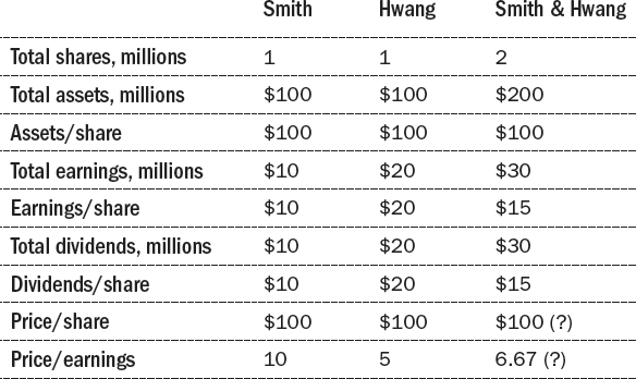
Yet, from the standpoint of Smith, earnings per share have jumped 50 percent, from $10 to $15. Conversely, from the standpoint of Hwang, earnings per share have fallen 25 percent, from $20 to $15. If the merged company is named Smith, investors might compare last year’s $10 earnings with this year’s $15, decide Smith is now a growth company, and apply a higher price-earnings ratio, pushing the price above $150 a share. Then Smith will be even better positioned to manufacture more earnings growth by acquiring more low-P/E companies. If, on the other hand, the new company is named Hwang, investors may compare this year’s $15 earnings with last year’s $20 and flee a disaster in the making. Both conclusions are wrong. The lesson is simple: Value investors should look at the reasons for earnings growth.

BOOK VALUE

The book value of a firm is the net worth shown on the accountants’ books. It is commonly calculated on a per-share basis, total assets minus liabilities, divided by the number of shares outstanding.

Book values are generally based on the cost of a firm’s assets, depreciated over time for presumed wear and tear. However, a firm’s value to shareholders is the cash that it generates, not the cost of its assets. A firm that loses money year after year is of little value to shareholders even if it costs billions to construct its money-losing buildings and equipment. (Imagine a tomato farm on top of Mount Everest.) Conversely, a high-technology company operating out of a garage can be worth millions of dollars even though its garage is only worth thousands.

TOBIN’S Q

James Tobin argued that we should look at how financial markets value a firm relative to the replacement cost of its assets:

Tobin’s q is larger or smaller than 1 depending on whether the firm’s profits are larger or smaller than the shareholders’ required return on their stock. If this sounds like economic value added, you’re right.

If a firm’s profits are persistently larger than shareholders’ required return, economic value added is positive and Tobin’s q is larger than 1. If profits are less than shareholders’ required return, economic value added is negative and Tobin’s q is less than 1.

Tobin argues that a firm should invest in new buildings and equipment if the stock market will value the investment at more than its cost (that is, if its q ratio is greater than 1). Put more plainly, the appropriate question a firm should ask is whether, if the firm were to sell shares in its expansion, it could raise enough money to cover the cost.

The persuasive logic can be illustrated by a home builder’s calculation. It only makes sense to build homes if the potential market value exceeds the construction cost. The same reasoning applies to all corporate investment. A firm should compare the cost of its investments with the value that financial markets will place on these investments. If the market value is larger than the cost (q greater than 1), shareholders want the firm to make this investment, gladly giving up a dollar of dividends in exchange for a two-dollar increase in the value of their stock.

If a firm’s market value is less than the replacement cost of its assets (q less than 1), the firm is worth more dead than alive, and it should sell its assets and distribute the proceeds as dividends. Shareholders prefer two dollars of dividends to one dollar of market value.

WHAT DETERMINES Q?

How can assets be valued in financial markets at other than their replacement cost? Assets are of value to shareholders only to the extent they generate profits. It matters not at all that a factory cost $1 billion to build if it doesn’t make a dime of profits. For a factory to be worth what it costs shareholders, it must earn the shareholders’ required return.

Consider a restaurant that would cost $1 million to build and earn a constant 20 percent annual profit, $200,000, forever. All earnings are paid out as dividends. How much will investors pay for a $200,000 annual dividend? If Treasury bonds pay 5 percent, perhaps stock in a risky restaurant is priced to yield 10 percent. Using the JBW equation in Chapter 6 with no growth, the restaurant’s value is $2 million:

Valued at $2 million, the $200,000 annual dividend gives investors their 10 percent required return. The market value of the restaurant is twice its cost of construction (q = 2) and the restaurant is worth building because its 20 percent profit is larger than the investors’ 10 percent required return.

If, on the other hand, the investors’ required return is 25 percent, then the market value is only $800,000:

Now q = 0.8 and the restaurant is not worth building. Investors require a 25 percent return on their stock, but the restaurant earns only 20 percent on its cost. The stock must be valued at less than cost to give investors their requisite return.

USING Q TO PREDICT THE MARKET

A New York Times article titled “A New Way to Measure an Exhausted Bull” began: “Is the q ratio signaling that the end is near for this great bull market? The what? If you’re an economist, you didn’t even ask the second question.” The article went on to point out that q was 1.7 at that time and quoted a British consulting firm: “Professor Tobin received a Nobel prize for his work, and the U.S. stock market may thus be said to be making a bet of approximately $3 trillion that he should return his laurels. I expect him to be justified in keeping them.”

This bearish consultant evidently believed that market values were too high because they were 1.7 times replacement cost, rather than equal to replacement cost. The $3 trillion figure was the difference between market value and replacement cost.

However, Tobin’s q need not equal 1. The value of q could be 1.7, or even higher, if profit rates are higher than shareholder required returns. In our restaurant example, there is a compelling reason why q equals 2 and no reason why it should equal 1.

It turned out that the bull market was not exhausted. After the New York Times article appeared, the S&P went up 26 percent over the next twelve months and doubled over the next three years. Tobin’s q helps us understand why the stock market goes up or down, but it is not necessarily a tool for picking $100 bills up off the sidewalk.

VALUE STOCKS

There is considerable evidence of abnormal returns from “value” stocks that have low prices relative to dividends, earnings, and book value. Mechanical rules are no guarantee of success, but these valuation metrics have the virtue of cultivating a contrarian approach to investing. Value investing and contrarian investing are often two sides of the same coin. When investors are fearful and contrarian investors look to pounce, stock prices are low relative to dividends, earnings, and book value, and these bargain prices attract value investors. Greed, on the other hand, which is a sell sign for contrarian investors, fuels high stock prices that scare off value investors.

Eugene Fama and others who believe that the market never makes a mistake argue that the abnormal returns from value strategies must be risk premiums. Therefore, value strategies must be risky—even if the only evidence we have of their riskiness is that they are profitable. Skeptics dismiss this reasoning as circular and argue that animal spirits and other market noise create profitable opportunities for contrarians and value investors.

THE DOGS OF THE DOW

Michael B. O’Higgins was an early and enthusiastic advocate of a strategy with the memorable name: the Dogs of the Dow. At the beginning of each year, calculate the dividend yield (dividend divided by price) for each of the thirty stocks in the Dow Jones Industrial Average and invest in the ten stocks with the highest dividend yields. These stocks are evidently out of favor, in that their prices are low relative to dividends—hence the label Dogs of the Dow. Writing in 1991, O’Higgins reported that the Dogs had outperformed the market for decades.

One explanation is the contrarian idea that investors overreact to bad news and their overreaction causes stock prices to fall too far, so that out-of-favor stocks are bargains. Another explanation is that a bird in the hand is worth two in the bush; that is, it is better to have a dividend in your pocket than dreams of capital gains at the end of a rainbow. Or perhaps it is just a coincidence uncovered by ransacking the data.

If it is just data mining, then it should do poorly with fresh data. In the twenty years after the Dogs of the Dow theory was first reported, the strategy had an annual return of 10.8 percent, the same as the Dow as a whole, but better than the S&P 500’s 9.6 percent. Solid, but not spectacular. Perhaps the Dogs of the Dow are not as far out of favor as are dogs not in the Dow.

LOW PRICE-EARNINGS RATIOS

Several studies have found that stocks with low P/Es outperform stocks with high P/Es. For instance, Benjamin Graham divided the Dow Jones Industrials into the ten highest, ten middle, and ten lowest P/E ratios. For every five-year holding period between 1937 and 1969, the low P/E stocks outperformed the middle P/E stocks, which outperformed the high P/E stocks. If $10,000 had been invested and reinvested every five years in the ten stocks with the lowest P/E ratios at that time, it would have grown to more than $100,000 by 1969, more than twice the amount accumulated by investing and reinvesting in the ten highest P/E stocks.

LOW PRICE-BOOK RATIOS

Another plausible identifier of out-of-favor stocks is the ratio of the stock price to book value. One study calculated the ratio of market value to book value for the S&P 500 on January 1 of each of the forty-five years from 1950–1994. The years were then divided into two categories, depending on the beginning-of-year ratio of market value to book value: 1) the twenty-two years with the highest ratios and 2) the twenty-two years with the lowest ratios. (The median year was discarded.) The years with low beginning-of-year price-book ratios had an average return of 20 percent, the years with high price-book ratios 6 percent.

Similar results have been found for individual stocks. Even Fama, perhaps the most enthusiastic proponent of the efficient market hypothesis, has admitted that stocks with low price-book ratios beat the market. His explanation is unconvincing. He argues that because markets are efficient (might as well assume what you are trying to prove), low price-book stocks must have risks that we do not understand but investors fear.

A more persuasive explanation is that Mr. Market’s prices fluctuate more than intrinsic values. When Mr. Market’s prices are high relative to benchmarks like dividends, earnings, and book value, his prices are probably too high. When Mr. Market’s prices are low relative to these benchmarks, they are probably too low.

SMALL CAPITALIZATION STOCKS

It is not profitable for large institutions to do expensive research on small companies because any attempt to buy a substantial number of shares will drive the price upward and a later sale will force the price down. If small stocks are neglected, they might also be cheap.

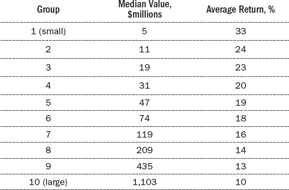
Several studies have found that firms with a small total market value, called small capitalization or small-cap firms, have significantly outperformed larger companies. One study considered the performance of ten portfolios revised annually by dividing 2,000 stocks into ten groups based on their total market value at the time. The subsequent annual rates of return, neglecting transaction costs, are in Table 7-4 and show that small-cap portfolios consistently outperformed large-cap portfolios.

Fama has acknowledged that small-cap stocks have outperformed large caps. And he has again reached for the unconvincing explanation that small-cap stocks must be riskier than large-cap stocks; we just don’t know how to measure these risks.

SCUTTLEBUTT

Philip Fisher touted “scuttlebutt”—talking to a company’s managers, employees, customers, and suppliers and to knowledgeable people in the industry in order to identify able companies with good growth prospects. In an efficient market, if it is well known that a company is great, its stock should trade at a price that reflects its greatness. However, Fisher’s scuttlebutt might be justified by the argument that Wall Street is fixated with numbers and it takes more than numbers to identify a great company.

Since 1983, Fortune magazine has published an annual list of the most-admired companies based on surveys of thousands of executives, directors, and securities analysts. The top 10 (in order) in 2016 were Apple, Alphabet (Google), Amazon, Berkshire Hathaway, Walt Disney, Starbucks, Southwest Airlines, FedEx, Nike, and General Electric.

I looked at the performance of a stock portfolio of Fortune’s top-10 companies from 1983 through 2015. In one set of calculations, the trading day for the Fortune portfolio was the official publication date, which is a few days after the magazine goes on sale. I also looked at trading days one to four weeks after the publication date. On the trading day each year, the Fortune portfolio was reinvested in that year’s ten most admired companies.

The Fortune strategy beat the S&P 500 soundly, with respective annual returns of 15 percent versus 10 percent. It is unlikely that this difference is some sort of risk premium since the companies selected as America’s most admired are large and financially sound and their stocks are likely to be viewed by investors as very safe. By the usual statistical measures, they were safer. Nor is the difference in returns due to the extraordinary performance of a few companies. Nearly 60 percent of the Fortune stocks beat the S&P 500.

This is a clear challenge to the efficient market hypothesis since Fortune’s list is readily available public information. I have no compelling explanation for this anomaly. Perhaps Fisher was right. The way to beat the market is to focus on scuttlebutt—intangibles that don’t show up in a company’s balance sheet—and the Fortune survey is the ultimate scuttlebutt.